Control Systems Technology Lab
Lecture Notes
Nicanor Quijano
The Ohio State University
Department of Electrical and Computer Engineering
2015 Neil Avenue, Columbus Ohio, 43210, USA
June 20, 2005
1
General Comments
• There are 9 laboratories, and each of them will cost 8% of the final grade (the pre-lab is 40% and the lab-procedure is 60% of the total 8% for an specific lab). The final will be 28% of the final grade.
• The students will be rotated in different groups. Since we have eight students per section, the idea is to rotate all of them in different groups, in order to avoid any kind of conflicts between them.
• Since in each lab the student will have a different partner, it is required to hand in a pre-lab per person. However, the lab procedures required to be handed in the next session could be done independently or per group.
• The last week of classes will be devoted to the final. This lab practical serves as a final examination for ECE557. In this lab, we want to test the knowledge of the students in classical control design, Simulink, and dSPACE. This final will be based on the knowledge acquired through the quarter, and it is individual.
• The students should read the Lab manual before every lab session, and hand in the pre-lab assignment. Sometimes, I will do a quiz at the beginning of the lab, asking simple questions regarding the lab procedures and the last lab. I will announce these quices one week in advance.
• How should I save my files?? Normally all the students will have access to their z drive on the ECE department. Therefore, the login will be the same as the one that any of the students does at CL260. With the access to these drives, the students can save their files used in the lab, and also the data necessary to generate a lab report.
• There are many ways to save data. One is described in the manual. There are others, and if you are curious, you can go to Professor Kevin Passino’s webpage under ECE758, and you will see another dSPACE tutorial developed before this one, and used for that course (see Section 4 for the URL).
2
Laboratory 1
2.1
Introduction to Control Systems
The following sentences were extracted from [3, 2].
• Control engineering is based on the foundations of feedback theory and linear system analysis, and it integrates the concepts of network theory and communication theory.
• The word “feedback” is a 20th century neologism introduced in the 1920s by radio engineering to describe parasitic, positive feeding back of the signal from the output of an amplifier to the input circuit.
• A control system is an interconnection of components forming a system configuration that will provide a desired system response.
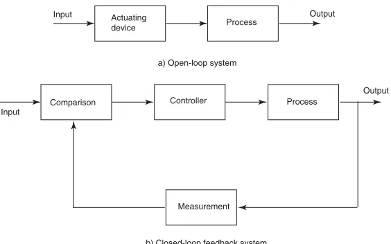
• Figure 1 shows the input-output relation that might exist between different blocks as it is shown. Figure 1a) shows the open-loop configuration that utilizes an actuator in order to obtain a desired response, but the process does not need a feedback such as the one shown in Figure 1b).
Actuating
device Process
Input Output
a) Open-loop system
b) Closed-loop feedback system
Comparison Controller Process
Measurement Input
Output
Figure 1: Configurations.
2.2
History
The following selected historical developments of Control Systems is extracted from [3, 4].
• 1769: James Watt’s steam engine and governor is developed.
• 1868: Maxwell formulates a mathematical model for a governor control of a steam engine.
• 1927: Bode analyzes feedback amplifiers.
• 1932: Nyquist develops a method for analyzing the stability of systems.
• 1948: Evans developed the root locus technique.
• 1954: George Devol develops “programmed article transfer.” considered to be the first industrial robot design.
• 1970: State variable models and optimal control developed.
• 1980: Robust control system design widely studied.
2.3
Laboratory Procedures
In the first lab we use Simulink and dSPACE in order to identify a simulated unknown transfer function. For that, we use frequency domain system identification methods, in order to identify a second order system in the form
G(s) = kw
2
n
s2+ 2ζw
ns+w2n
where k is the DC gain, ζ is the damping ratio, and wn is the undamped natural frequency. The transfer function G(s) is the relationship in frequency domain between the output C(s), and the input R(s), in Figure 2.
G(s)
C(s)
R(s)
Figure 2: Single open-loop system. R(s) is the input,C(s) is the output, andG(s) is the transfer function that relates both input and output, everything in the frequency domain.
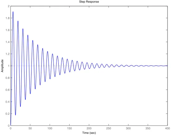
Without loss of generality, we will assume in the following analysis that k = 1. Figure 3 shows an example of the frequency response ofG(s). In this figure, we can see four important values: Mpw that is the maximum magnitude, and it occurs at the resonant frequency wr; also, we have that the system has a bandwidthwB, when the magnitude reaches -3 dB. This bandwidthwBis “a measure of a system’s ability to faithfully reproduce an input signal” [3]. Normally, this value is related to how fast the system can respond. IfwB increases, the rise time of the system will decrease. The maximum magnitude Mpw is related to the overshoot of the system to a step input (shown in Figure 4), and hence its value is closely related to the damping ratioζ. Ifζ≤ 1
√
2, then the magnitudeMr=Mpw can be computed as
Mr= 1
2ζ1−ζ2, ζ≤
1
√
2
where the units ofMr=Mpw are not in dB. Ifk is not equal to 1, then the magnitude of resonance is not anymoreMpw, but instead, it is the difference betweenMpw andM0= 20 log10k, i.e.,Mr=Mpw−M0. To computewn when ζ ≤ √12, we can use directly the resonance frequency wr, because this is related to the undamped natural frequency through
wr=wn
1−2ζ2, ζ≤ √1
2
As an example of what we have described so far, let us see how we can determine the values for G(s) in Figure 3. From this figure, we can see that wr= 0.5rad/sec, and thatMpw = 24.4dB = 10
24.4
20 = 16.6.
Therefore, applying the previous formulas, assuming thatζ≤ 1
√
2, we obtain
4M2
rζ
4
−4M2
rζ
2
+ 1 = 0
Solving this equation, we find that the roots are 0.9995,−0.9995, 0.0300, and −0.0300. Since the equation is valid only forζ≤ 1
√
2, we conclude that in this caseζ= 0.03. Finally, solving forwn, we have that
wn=
wr
1−2ζ2, ζ≤
1
√
2
60 50 40 30 20 10 0 10 20 30
Magnitude (dB)
10 1 100 101
180 135 90 45 0
Phase (deg)
Bode Diagram
Frequency (rad/sec)
20logMpw
3 dB
wr w
B
Figure 3: Magnitude and phase characteristics for the second-order systemG(s) = 0.25
s2+0.03s+0.25.
0 50 100 150 200 250 300 350 400
0 0.2 0.4 0.6 0.8 1 1.2 1.4 1.6 1.8 2
Step Response
Time (sec)
Amplitude
Figure 4: Step response for the second-order system G(s) = 0.25
s2+0.03s+0.25.
an input to this black box, and from dSPACE, we change the frequency of the sine wave every run, and we save the data just obtained. Then, we can draw a magnitude bode plot with these values, and we are going to obtain a figure similar to the on in Figure 3.
to pause the experiment. This RadioButton will allow the user to start and stop the experiment whenever he/she wants. It is better to do that, because the user will know exactly when the experiment started, and also it helps to have a complete set of data saved.
3
Laboratory 2
3.1
SAMPLING
“In the context of control and communication, sampling means that a continuous-time signal is replaced by a sequence of numbers, which represents the values of the signal at certain times.” [1].
In general, from Figure 5 [1], we have that the continuous signaly(t), that is produced by the process, is sampled and converted into a sequence of numbers by means of the ADC. After an algorithm or a decision process is taken into account, we take the output (that is again a sequence of numbers), and we need then to convert these numbers into a continuous signal. This reconstruction process is done via the DAC.
y(t) u(t)
t
t
t t
u[n] y[n]
PROCESS
COMPUTER A/D D/A
HOLD
SAMPLER
Figure 5: Process of taking a continuous-time signaly(t) that is generated by a process, and convert it into a sequence of numbersy[n]. The computer takes a decision that is converted into a sequence of numbers
u[n], which in turn is converted into the continuous-time signalu(t) that enters into the process.
We know that “very little is list by sampling a continuous-time signal if the sampling instants are suffi-ciently close, but much of the information about a signal can be lost if the sampling points are too far apart.” [1].
When we sample a given signal, we are creating at the same time signals with different frequencies. Let us say that we sample a signal at a frequency
ws= 2π Ts
whereTsis the sampling period. The new frequencies generated after the sampling are given by
wSa =kws±w
wherewSa is the sampled frequency,wis the frequency of the original signal that we sampled, andk is an integer number.
then there is no loss of information between the original signal and the sampled one. Mathematically this is known as the Nyquist sampling theorem, where wN is know as the Nyquist frequency, and normally is defined aswN = ws
2 .
“After sampling, a frequency thus cannot be distinguished from its aliases. The fundamental alias for a frequencyw1> wN = w2s is given by
w=|(w1+wN)mod(ws)−wN|
wheremod(x, y) =x−f loor(x y).y.
Example: f1= 0.1 Hz,f2= 0.9 Hz,fs= 1 Hz. One of the aliasing frequencies forf2 is given at
f =|mod(1.4,0.5)−0.5|=|0.4−0.5|= 0.1!!!
Figure 6 (taken from [1]) shows this effect, by using two different signals x1(t) = sin(2πf1t) and x2(t) =
−sin(2πf2t), with the given frequencies. This is an excellent example of who aliasing can affect the perfect
reconstruction of the signals.
0 1 2 3 4 5 6 7 8 9 10
−1 −0.8 −0.6
−0.4
−0.2
0 0.2 0.4 0.6 0.8 1
Figure 6: In this figure we see that two signalsx1(t) = sin(2πf1t) (dashed), andx2(t) =−sin(2πf2t) (solid).
If we sample both signals with a period of 1 second, the value after the sampling will be the same at all sampling instants.
4
Laboratory 3
This laboratory is self explanatory, and it does not require a lot of theory to develop previous the practice. However, we are going to consider a small change in the procedure to make the lab more efficient. The following changes have to be implemented during the practice.
• In page 37 of the laboratory procedures, they say that the simulation time should be 8 seconds. Instead of using this value, we are going to use “inf” for the “Stop time” on the “Solver” tab for the “Simulation Parameters.”
• On page 38, remember to set at 0 Volts the termination of DAC.
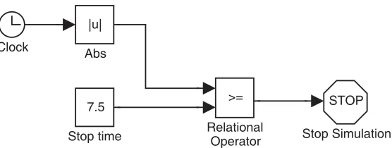
• At the end of page 38, they ask you to change the step input time to 7 seconds, and compile the model in order to acquire that value and run the experiment again. This is one way to do it, but clearly it is quite inefficient. What we are going to do is to add a couple of extra blocks as it is shown in Figure 7.
7.5
Stop time
STOP
Stop Simulation >=
Relational Operator Clock
|u|
Abs
Figure 7: This is the Simulink model of the elements that have to be added in Figure 3.6 to make more efficient your experiment.
As you can see, here we are adding five elements that will allow you to change the stop time from dSPACE. Therefore, instead of changing the step input from the step function, we are going to stop the simulation at the value given by the block “Stop time.” This block is a constant, hence you can associate a numeric input in the ControlDesk of dSPACE in order to change this value. The idea is that we do not need to compile the whole model again, that is a time consuming task.
• As in the other labs, there is something that is not mentioned in the procedures. You have to add a RadioButton in the ControlDesk of dSPACE in order to control the state of the simulation. On the “Tool window,” you will find the “Variable list” associated to the elements in your Simulink model. There, you will find the variable “simState” that you will drag and drop on the RadioButton developed to control the state of the simulation. Once you do that, double click on this element, and change the states in order that you associate “STOP” to a 0 state, and the state 2 to “START.” The state corresponding to 1 is “PAUSE” but you will not need to pause the experiment.
For another tutorial on dSPACE besides the one that you have in your lab procedure, go to: http://www.ece.osu.edu/˜passino/dSPACEtutorial.doc.pdf
5
Laboratory 4
There are many references where we can learn the basics for the root locus analysis. In the next few lines, we are going to take the ideas in [5].
5.1
STEADY-STATE ERRORS IN UNITY FEEDBACK CONTROL SYSTEMS
One useful way to characterize control systems, and that is the ability that the open loop transfer function has in order to follow different inputs (e.g., step input, ramp input, parabolic input, etc.). As we are going to see, the characterization of the systems in terms of the response of different inputs is useful in order to determine the magnitudes of the steady-state errors. In general, we have that the open loop transfer function
G(s) has the form
G(s) =K (s+z1)(s+z2). . .(s+zm) sN(s+p
1)(s+p2). . .(s+pn)
For instance, if we have the block diagram in Figure 8, we know that we can write the following transfer functions
C(s)
R(s) =
G(s) 1 +G(s)
E(s)
R(s) = 1 1 +G(s)
where R(s) represents the Laplace transform of the input, C(s) represents the Laplace transform of the output, E(s) represents the Laplace transform of the error, andG(s) represents the Laplace transform of the process. Therefore, the steady-state error is given by thefinal value theorem, we have that
ess= lim
t→∞e(t) = lims→0sE(s) = lims→0s
R(s) 1 +G(s)
Table 1 summarizes the steady-state errors for different inputs, and different type numbers.
ess Step Inputr(t) =u(t) Ramp Inputr(t) =t Parabolic Inputr(t) =t2
Type 0 1
1+K ∞ ∞
Type 1 0 1
K ∞
Type 2 0 0 1
K
Table 1: Steady-state errors for different inputs.
+
-
G(s)
R(s)
E(s)
C(s)
Figure 8: Block diagram for a unity feedback control system loop.
5.2
ROOT LOCUS ANALYSIS
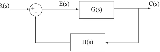
Suppose that we have a system in the form of Figure 9, where the transfer function G(s) has a parameter
K that represents the gain of the controller. This parameter is strictly positive, otherwise we would have a positive feedback case, which will lead us to change the angle condition in the next analysis. Therefore, without loss of generality, we are going to assume in what remains thatK >0.
+
-
G(s)
R(s)
E(s)
C(s)
H(s)
The transfer function of the system is given by
C(s)
R(s) =
G(s)
1 +G(s)H(s) (1)
And, from here, we obtain the characteristic equation given by,
1 +G(s)H(s) = 0 (2)
We can rearrange Equation (2) in order to let the parameter of interest appearing as the multiplying factor in the form
1 +K(s+z1)(s+z2). . .(s+zm)
(s+p1)(s+p2). . .(s+pn)
= 0
wheren > m, and of course,K >0 is the parameter of interest. This method is also applicable to systems that have parameters of interest other than the gain.
Basically, we have to follow a couple of steps in order to draw a root-locus. These steps are:
1. First, we need to locate the poles and zeros ofG(s)H(s) on thesplane. Normally we draw the poles with anxand the zeros witho.
2. Now, we start drawing the root loci on the real axis. Since the angle contribution of the complex-conjugates poles and zeros ofG(s)H(s) is 360◦ on the real axis. Then, we need to look only the poles
and zeros on the real axis. For that, we take a test point on the real axis, and if the total number of poles and zeros to the right of this test point is odd, then this point lies on a root locus.
3. Now, we determine the asymptotes of root loci
σa =−
pi−zi
n−m
β=±180(2n k+ 1) −m
where n is the number of finite poles ofG(s)H(s), mis the number of finite zeros ofG(s)H(s), and
k= 0,1, . . . , n−m−1.
4. The breakaway and break-in points can be found in the following ways:
1
σb+pi
= 1
σb+zi
or, suppose that the characteristic equation is given by
B(s) +KA(s) = 0
From this characteristic equation, we can derive the breakaway and break-in points by solving the next equation
dK ds =−
B′(s)A(s)−B(s)A′(s)
A2(s)
5. Determine the angle of departure,θDep (angle of arrival,θArr) of the root locus from a complex pole
(at a complex zero, respectively)
θDep = 180−αp+
αz
θArr = 180−αz+
αp
6. Now, we need to find the points where the root loci cross (or may cross) the imaginary axis. For that, we use the Routh-Hurwitz’s stability criterion, and then, settings=jwin the characteristic equation, we solve the equations for the real and imaginary components, and obtain thewandKvalues. These values will give us the frequency wwhere the root loci cross the imaginary axis, and the critical gain
K that will give us this result.
7. Now, in order to get a better sketch of the root locus, we need to take a couple of test point.
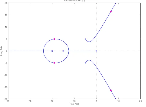
Some of the cases for the root locus can be seen in Figures 10 to 15.
−30 −25 −20 −15 −10 −5 0 5 10
−20 −15 −10 −5 0 5 10 15 20
Imag Axis
Real Axis Root Locus Editor (C)
Figure 10: Root locus for the transfer functionG(s) = 1
s3+15s2+50s.
−15 −10 −5 0 5
−15 −10 −5 0 5 10 15
Real Axis
Imag Axis
Root Locus Editor (C)
Figure 11: Root locus for the transfer functionG(s) = 1
−4 −3 −2 −1 0 1 2 3 4 −2
−1.5 −1 −0.5 0 0.5 1 1.5 2
Real Axis
Imag Axis
Root Locus Editor (C)
Figure 12: Root locus for the transfer functionG(s) = 1
s4+4s3+6s2+4s.
−4 −3 −2 −1 0 1 2 3 4
−4 −3 −2 −1 0 1 2 3 4
Real Axis
Imag Axis
Root Locus Editor (C)
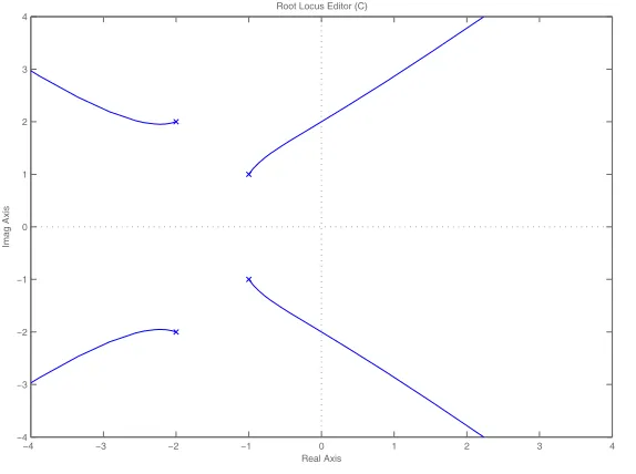
Figure 13: Root locus for the transfer functionG(s) = 1
s4+6s3+18s2+24s+16.
6
Laboratory 5
There are many references where we can learn the basics for the lag compensator. In the next few lines, we are going to take the ideas in [3].
6.1
GENERAL COMMENTS
• Bode design method does not eliminate steady-state error because it only deals with improving the phase margin of the system; in order to eliminate steady-state error, a gain is needed with the com-pensator and this is done in the root locus design method.
−40 −30 −20 −10 0 10 20 30 −40
−30 −20 −10 0 10 20 30 40
Real Axis
Imag Axis
Root Locus Editor (C)
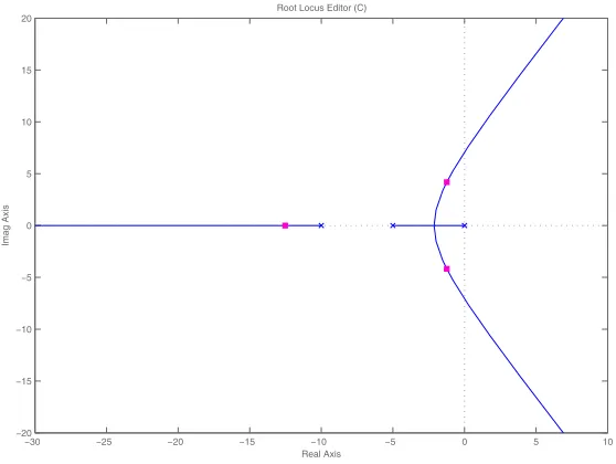
Figure 14: Root locus for the transfer functionG(s) = 1
s4+30s3+250s2+1000s.
−40 −30 −20 −10 0 10 20
−20 −15 −10 −5 0 5 10 15 20
Real Axis
Imag Axis
Root Locus Editor (C)
Figure 15: Root locus for the transfer functionG(s) = s+20
s4+25s3+200s2+750s.
settling time, therefore aggressive gains should be avoided in favor of a small gain that assures only steady-state error. The gain should not exceed a value of 5!!
7
FINAL ECE 557
• The idea of the lab final is to evaluate most of the concepts that the students learned during the quarter.
he/she considers important. This sheet will be handed in at the end of the exam.
References
[1] Karl J. ˚Astr¨om and Bj¨orn Wittenmark. Computer Controlled Systems. Prentice Hall, New Jersey, NJ, 1997.
[2] Stuart Bennet. A brief history of automatic control. IEEE Control Systems Magazine, 16(3):17–25, June 1996.
[3] Richard C. Dorf and Robert H. Bishop. Modern Control Systems. Addison-Wesley, Reading, MA, 1995.
[4] Gene F. Franklin, J. David Powell, and Abbas Emami-Naeini. Feedback Control of Dynamic Systems. Addison-Wesley, Reading, MA, 1994.
![Figure 5: Process of taking a continuous-time signal yu(t) that is generated by a process, and convert it intoa sequence of numbers y[n]](https://thumb-ap.123doks.com/thumbv2/123dok/619157.164695/5.612.166.450.259.460/figure-process-continuous-generated-process-convert-sequence-numbers.webp)
![Figure 6 (taken from [1]) shows this effect, by using two different signals x1(t) = sin(2πf1t) and x2(t) =−sin(2πf2t), with the given frequencies](https://thumb-ap.123doks.com/thumbv2/123dok/619157.164695/6.612.166.445.292.513/figure-taken-shows-eect-using-dierent-signals-frequencies.webp)