Analytic Number Theory
Andrew Granville1 Introduction
What is number theory? One might have thought that it was simply the study of numbers, but that is too broad a definition, since numbers are almost ubiqui-tous in mathematics. To see what distinguishes num-ber theory from the rest of mathematics, let us look at the equation x2+y2 = 15 925, and consider whether it has any solutions. One answer is that it certainly does: indeed, the solution set forms a circle of radius
√
15 925 in the plane. However, a number theorist is interested inintegersolutions, and now it is much less obvious whether any such solutions exist.
A useful first step in considering the above question is to notice that 15 925 is a multiple of 25: in fact, it is 25×637. Furthermore, the number 637 can be decomposed further: it is 49×13. That is, 15 925 = 52×72×13. This information helps us a lot, because
if we can find integersaandbsuch thata2+b2= 13,
then we can multiply them by 5×7 = 35 and we will have a solution to the original equation. Now we notice that a = 2 and b= 3 works, since 22+ 32 =
13. Multiplying these numbers by 35, we obtain the solution 702+ 1052= 15 925 to the original equation.
As this simple example shows, it is often useful to decompose positive integers multiplicatively into components that cannot be broken down any further. These components are calledprime numbers, and the fundamental theorem of arithmetic states that every positive integer can be written as a product of primes in exactly one way. That is, there is a one-to-one correspondence between positive integers and finite products of primes. In many situations we know what we need to know about a positive integer once we have decomposed it into its prime factors and under-stood those, just as we can understand a lot about molecules by studying the atoms of which they are composed. For example, it is known that the equation x2+y2=nhas an integer solution if and only if every prime of the form 4m+ 3 occurs an even number of times in the prime factorization of n. (This tells us,
equationx +y = 13 475, since 13 475 = 5 ×7 ×11, and 11 appears an odd number of times in this prod-uct.)
Once one begins the process of determining which integers are primes and which are not, it is soon appar-ent that there are many primes. However, as one goes further and further, the primes seem to consist of a smaller and smaller proportion of the positive inte-gers. They also seem to come in a somewhat irregular pattern, which raises the question of whether there is any formula that describes all of them. Failing that, can one perhaps describe a large class of them? We can also ask whether there are infinitely many primes? If there are, can we quickly determine how many there are up to a given point? Or at least give a good esti-mate for this number? Finally, when one has spent long enough looking for primes, one cannot help but ask whether there is a quick way of recognizing them. This last question is discussed in computational number theory; the rest motivate this article.
Now that we have discussed what marks number theory out from the rest of mathematics, we are ready to make a further distinction: betweenalgebraic and analytic number theory. The main difference is that in algebraic number theory (which is the main topic ofalgebraic numbers) one typically considers ques-tions with answers that are given by exact formulas, whereas in analytic number theory, the topic of this article, one looks forgood approximations. For the sort of quantity that one estimates in analytic number the-ory, one does not expect an exact formula to exist, except perhaps one of a rather artificial and unillu-minating kind. One of the best examples of such a quantity is one we shall discuss in detail: the number of primes less than or equal tox.
Since we are discussing approximations, we shall need terminology that allows us to give some idea of the quality of an approximation. Suppose, for exam-ple, that we have a rather erratic functionf(x) but are able to show that, oncexis large enough,f(x) is never bigger than 25x2. This is useful because we
under-stand the functiong(x) = x2 quite well. In general,
if we can find a constantc such that|f(x)| cg(x) for everyx, then we writef(x) =O(g(x)). A typical usage occurs in the sentence “the average number of prime factors of an integer up toxis log logx+O(1)”; in other words, there exists some constantc >0 such
that|the average−log logx|concexis sufficiently large.
We writef(x)∼g(x) if limx→∞f(x)/g(x) = 1; and
alsof(x)≈g(x) when we are being a little less precise, that is, when we want to say thatf(x) andg(x) come close whenxis sufficiently large, but we cannot be, or do not want to be, more specific about what we mean by “come close.”
It is convenient for us to use the notation for sums and
for product. Typically we will indicate beneath the symbol what terms the sum, or product, is to be taken over. For example,
m2will be a sum
over all integersmthat are greater than or equal to 2, whereas
pprime will be a product over all primesp.
2 Bounds for the Number of Primes
Ancient Greek mathematicians knew that there are infinitely many primes. Their beautiful proof by con-tradiction goes as follows. Suppose that there are only finitely many primes, say k of them, which we will denote byp1, p2, . . . , pk. What are the prime factors of
p1p2· · ·pk+ 1? Since this number is greater than 1 it
must have at least one prime factor, and this must be pjfor somej(sinceall primes are contained amongst
p1, p2, . . . , pk). But then pj divides both p1p2· · ·pk
andp1p2· · ·pk+1, and hence their difference, 1, which
is impossible.
Many people dislike this proof, since it does not actually exhibit infinitely many primes: it merely shows that there cannot be finitely many. It is more or less possible to correct this deficiency by defin-ing the sequence x1 = 2, x2 = 3 and then xk+1 =
x1x2· · ·xk+ 1 for eachk2. Then eachxkmust
con-tain at least one prime factor,qksay, and these prime
factors must be distinct, since ifk < ℓ, thenqkdivides
xkwhich dividesxℓ−1, whileqℓdividesxℓ. This gives
us an infinite sequence of primes.
In the seventeenth century Euler gave a differ-ent proof that there are infinitely many primes, one that turned out to be highly influential in what was to come later. Suppose again that the list of primes is p1, p2, . . . , pk. As we have mentioned, the
funda-mental theorem of arithmetic implies that there is a one-to-one correspondence between the set of all inte-gers and the set of products of the primes, which, if those are the only primes, is the set {pa1
1 pa22· · ·p ak
k :
a1, a2, . . . , ak 0}. But, as Euler observed, this
implies that a sum involving the elements of the first set should equal the analogous sum involving the ele-ments of the second set:
n1 na positive integer
1
The last equality holds because each sum in the second-last line is the sum of a geometric progres-sion. Euler then noted that if we take s = 1, the right-hand side equals some rational number (since each pj > 1) whereas the left-hand side equals ∞.
This is a contradiction, so there cannot be finitely many primes. (To see why the left-hand side is infi-nite when s = 1, note that (1/n) nn+1(1/t) dt since the function 1/t is decreasing, and therefore N−1
n=1(1/n)
N
1 (1/t) dt= logN which tends to∞
asN→ ∞.)
During the proof above, we gave a formula for n−s under the false assumption that there are only
finitely many primes. To correct it, all we have to do is rewrite it in the obvious way without that assumption:
n1 na positive integer
1
Now, however, we need to be a little careful about whether the two sides of the formula converge. It is safe to write down such a formula when both sides are absolutely convergent, and this is true when s > 1. (An infinite sum or product isabsolutely convergentif the value does not change when we take the terms in any order we want.)
Like Euler, we want to be able to interpret what happens to (1) whens= 1. Since both sides converge and are equal when s > 1, the natural thing to do is consider their common limit as s tends to 1 from above. To do this we note, as above, that the left-hand side of (1) is well approximated by
so it diverges ass→1+. We deduce that
pprime
1−1p
= 0. (2)
Upon taking logarithms and discarding negligible terms, this implies that
pprime
1
p=∞. (3)
So how numerous are the primes? One way to get an idea is to determine the behaviour of the sum analogous to (3) for other sequences of integers. For instance,
n11/n
2 converges, so the primes are, in
this sense, more numerous than the squares. This argument works if we replace the power 2 by any s >1, since then, as we have just observed, the sum
n11/n
s is about 1/(s
−1) and in particular con-verges. In fact, since
n11/n(logn)
2 converges, we
see that the primes are in the same sense more numer-ous than the numbers{n(logn)2:n1}, and hence
there are infinitely many integers x for which the number of primes less than or equal to x is at least x/(logx)2.
Thus, there seem to be primes in abundance, but we would also like to verify our observations, made from calculations, that the primes constitute a smaller and smaller proportion of the integers as the integers become larger and larger. The easiest way to see this is to try to count the primes using the “sieve of Eratos-thenes.” In the sieve of Eratosthenes one starts with all the positive integers up to some number x. From these, one deletes the numbers 4, 6, 8 and so on—that is, all multiples of 2 apart from 2 itself. One then takes the first undeleted integer greater than 2, which is 3, and deletes allits multiples—again, not including the number 3 itself. Then one removes all multiples of 5 apart from 5, and so on. By the end of this process, one is left with the primes up tox.
This suggests a way to guess at how many there are. After deleting every second integer up toxother than 2 (which we call “sieving by 2”) one is left with roughly half the integers up to x; after sieving by 3, one is left with roughly two-thirds of those that had remained; continuing like this we expect to have about
x
py
1−1p
(4)
integers left by the time we have sieved with all the primes up toy. Oncey=√x the undeleted integers
are 1 and the primes up to x, since every composite has a prime factor no bigger than its square root. So, is (4) a good approximation for the number of primes up toxwheny=√x?
To answer this question, we need to be more pre-cise about what the formula in (4) is estimating. It is supposed to approximate the number of integers up toxthat have no prime factors less than or equal to y, plus the number of primes up toy. The so-called inclusion–exclusion principlecan be used to show that the approximation given in (4) is accurate to within 2k, wherekis the number of primes less than or equal
to y. Unless k is very small, this error term of 2k is
far larger than the quantity we are trying to estimate, and the approximation is useless. It is quite good ifk is less than a small constant times logx, but, as we have seen, this is far less than the number of primes we expect up to y if y ≈ √x. Thus it is not clear whether (4) can be used to obtain a good estimate for the number of primes up to x. What we can do, however, is use this argument to give an upper bound for the number of primes up tox, since the number of primes up toxis never more than the number of inte-gers up toxthat are free of prime factors less than or equal toy, plus the number of primes up toy, which is no more than 2k plus the expression in (4).
Now, by (2), we know that as y gets larger and larger the product
py(1−1/p) converges to zero.
Therefore, for any small positive numberεwe can find aysuch that
py(1−1/p)< ε/2. Since every term
in this product is at least 1/2, the product is at least 1/2k. Hence, for any x 22k our error term, 2k, is no bigger than the quantity in (4), and therefore the number of primes up toxis no larger than twice (4), which, by our choice of y, is less than εx. Since we were free to makeε as small as we liked, the primes are indeed a vanishing proportion of all the integers, as we predicted.
with primepwe supposed that roughly 1 in everypof the remaining integers were deleted: a careful analy-sis yields that this can be justified when p is small, but that this becomes an increasingly poor approxi-mation of what really happens for largerp; in fact (4) does not give a correct approximation onceyis bigger than a fixed power of x. So what goes wrong? In the hope that the proportion is roughly 1/plies the unspo-ken assumption that the consequences of sieving byp are independent of what happened with the primes smaller thanp. But if the primes under consideration are no longer small, then this assumption is false. This is one of the main reasons that it is hard to estimate the number of primes up tox, and indeed similar dif-ficulties lie at the heart of many related problems.
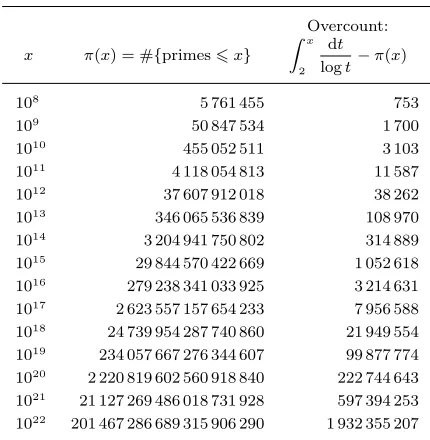
One can refine the bounds given above but they do not seem to yield an asymptotic estimate for the primes (that is, an estimate which is correct to within a factor that tends to 1 asxgets large). The first good guesses for such an estimate emerged at the begin-ning of the nineteenth century, none better than what emerges from Gauss’s observation, made when study-ing tables of primes up to three million, at 16 years of age, that “the density of primes at aroundxis about 1/logx.” Interpreting this, we guess that the number of primes up toxis about
x
n=2
1 logn ≈
x
2
dt logt.
Let us compare this prediction (rounded to the nearest integer) with the latest data on numbers of primes, dis-covered by a mixture of ingenuity and computational power. Table 1 shows the actual numbers of primes up to various powers of 10 together with the differ-ence between these numbers and what Gauss’s formula gives. The differences are far smaller than the numbers themselves, so his prediction is amazingly accurate. It does seem always to be an overcount, but since the width of the last column is about half that of the cen-tral one it appears that the difference is something like√x.
In the 1930s, the great probability theorist, Cram´er, gave a probabilistic way of interpreting Gauss’s predic-tion. We can represent the primes as a sequence of 0s and 1s: Putting a “1” each time we encounter a prime, and a “0” otherwise, we obtain, starting from 3, the sequence 1,0,1,0,1,0,0,0,1,0,1, . . .. Cram´er’s idea is to suppose that this sequence, which represents
Table 1 Primes up to variousx, and the overcount in Gauss’s prediction.
Overcount:
x π(x) = #{primesx} x
2
dt logt−π(x)
108 5 761 455 753
109 50 847 534 1 700
1010 455 052 511 3 103
1011 4 118 054 813 11 587
1012
37 607 912 018 38 262 1013
346 065 536 839 108 970 1014 3 204 941 750 802 314 889
1015 29 844 570 422 669 1 052 618
1016 279 238 341 033 925 3 214 631
1017
2 623 557 157 654 233 7 956 588 1018
24 739 954 287 740 860 21 949 554 1019 234 057 667 276 344 607 99 877 774
1020 2 220 819 602 560 918 840 222 744 643
1021 21 127 269 486 018 731 928 597 394 253
1022 201 467 286 689 315 906 290 1 932 355 207
the primes, has the same properties as a “typical” sequence of 0s and 1s, and to use this principle to make precise conjectures about the primes. More pre-cisely, letX3, X4, . . . be an infinite sequence of
ran-dom variablestaking the values 0 or 1, and let the variableXnequal 1 with probability 1/logn(so that
it equals 0 with probability 1−1/logn). Assume also that the variables are independent, so for each m knowledge about the variables other than Xm tells
us nothing aboutXm itself. Cram´er’s suggestion was
that any statement about the distribution of 1s in the sequence that represents the primes will be true if and only if it is true with probability 1 for his random sequences. Some care is needed in interpreting this statement: for example, with probability 1 a random sequence will contain infinitely many even numbers. However, it is possible to formulate a general princi-ple that takes account of such examprinci-ples.
Here is an example of a use of the Gauss–Cram´er model. With the help of thecentral limit theorem one can prove that, with probability 1, there are
x
2
dt logt+O(
√
xlogx)
representing primes, and so we predict that
just as the table suggests.
The Gauss–Cram´er model provides a beautiful way to think about distribution questions concerning the prime numbers, but it does not give proofs, and it does not seem likely that it can be made into such a tool; so for proofs we must look elsewhere. In analytic number theory one attempts to count objects that appear naturally in arithmetic, yet which resist being counted easily. So far, our discussion of the primes has concentrated on upper and lower bounds that follow from their basic definition and a few elemen-tary properties—notably the fundamental theorem of arithmetic. Some of these bounds are good and some not so good. To improve on these bounds we shall do something that seems unnatural at first, and reformu-late our question as a question about complex func-tions. This will allow us to draw on deep tools from analysis.
3 The “Analysis” in Analytic Number Theory
These analytic techniques were born in an 1859 mem-oir of Riemann, in which he looked at the function that appears in the formula (1) of Euler, but with one crucial difference: now he considered complex values of s. To be precise, he defined what we now call the Riemann zeta function as follows:
ζ(s) :=
n1
1 ns.
It can be shown quite easily that this sum converges whenever the real part of s is greater than 1, as we have already seen in the case of real s. However, one of the great advantages of allowing complex values of s is that the resulting function is holomorphic, and we can use a process of analytic continuation (these terms are discussed in Section ?? of some funda-mental mathematical definitions) to make sense ofζ(s) for everysapart from 1. (A similar but more elementary example of this phenomenon is the infinite series
n0z
n, which converges if and only if |z|<1. However, when it does converge, it equals 1/(1−z), and this formula defines a holomorphic function that
is defined everywhere exceptz= 1.) Riemann proved the remarkable fact that confirming Gauss’s conjec-ture for the number of primes up toxis equivalent to gaining a good understanding of the zeros of the func-tionζ(s)—that is, of the values ofsfor whichζ(s) = 0. Riemann’s deep work gave birth to our subject, so it seems worthwhile to at least sketch the key steps in the argument linking these seemingly unconnected topics. Riemann’s starting point was Euler’s formula (1). It is not hard to prove that this formula is valid when sis complex, as long as its real part is greater than 1, so we have
If we take the logarithm of both sides and then differ-entiate, we obtain the equation
−ζ
We need some way to distinguish between primesp xand primesp > x; that is, we want to count those primespfor whichx/p1, but not those withx/p < 1. This can be done using thestep functionthat takes the value 0 fory <1 and the value 1 for y >1 (so that its graph looks like a step). Aty= 1, the point of discontinuity, it is convenient to give the function the average value,1
2. Perron’s formula, one of the big tools
of analytic number theory. describes this step function by an integral, as follows. For anyc >0,
1
The integral is a path integral along a vertical line in the complex plane: the line consisting of all points c+ it with t ∈ R. We apply Perron’s formula with y=x/pm, so that we count the term corresponding
We can justify swapping the order of the sum and the integral if c is taken large enough, since every-thing then converges absolutely. Now the left-hand side of the above equation is not counting the number of primes up toxbut rather a “weighted” version: for each prime p we add a weight of logp to the count. It turns out, though, that Gauss’s prediction for the number of primes up to x follows so long as we can show thatxis a good estimate for this weighted count whenxis large. Notice that the sum in (6) is exactly the logarithm of the lowest common multiple of the integers less than or equal tox, which perhaps explains why this weighted counting function for the primes is a natural function to consider. Another explanation is that if the density of primes near p is indeed about 1/logp, then multiplying by a weight of logpmakes the density everywhere about 1.
If you know some complex analysis, then you will know that Cauchy’s residue theorem allows one to evaluate the integral in (6) in terms of the “residues” of the integrand (ζ′(s)/ζ(s))(xs/s), that is, the poles
of this function. Moreover, for any functionf that is analytic except perhaps at finitely many points, the poles off′(s)/f(s) are the zeros and poles off. Each
pole off′(s)/f(s) has order 1, and the residue is
sim-ply the order of the corresponding zero, or minus the order of the corresponding pole, off. Using these facts we can obtain theexplicit formula
pprime, m1 pmx
logp=x− ρ:ζ(ρ)=0
xρ
ρ − ζ′(0)
ζ(0). (7)
Here the zeros of ζ(s) are counted with multiplicity: that is, if ρ is a zero of ζ(s) of orderk, then there are k terms forρ in the sum. It is astonishing that there can be such a formula, an exact expression for the number of primes up to xin terms of the zeros of a complicated function: you can see why Riemann’s work stretched people’s imagination and had such an impact.
Riemann made another surprising observation which allows us to easily determine the values ofζ(s) on the left-hand side of the complex plane (where the function is not naturally defined). The idea is to multi-plyζ(s) by some simple function so that the resulting productξ(s) satisfies thefunctional equation
ξ(s) =ξ(1−s) for alls. (8)
He determined that this can be done by taking ξ(s) :=1
2s(s−1)π −s/2Γ(1
2s)ζ(s). Here Γ(s) is the
famousgamma function, which equals the factorial function at positive integers (that is,Γ(n) = (n−1)!), and is well-defined and continuous for all others.
A careful analysis of (1) reveals that there are no zeros ofζ(s) with Re(s)>1. Then, with the help of (8), we can deduce that the only zeros of ζ(s) with Re(s)<0 lie at the negative even integers−2,−4, . . . (the “trivial zeros”). So, to be able to use (7), we need to determine the zeros inside thecritical strip, the set of allssuch that 0Re(s)1. Here Riemann made yet another extraordinary observation which, if true, would allow us tremendous insight into virtually every aspect of the distribution of primes.
The Riemann hypothesis. If 0 Re(s) 1 and ζ(s) = 0, then Re(s) = 12.
It is known that there are infinitely many zeros on the line Re(s) = 1
2, crowding closer and closer together
as we go up the line. The Riemann hypothesis has been verified computationally for the ten billion zeros of lowest height (that is, with|Im(s)|smallest), it can be shown to hold for at least 40% of all zeros, and it fits nicely with many different heuristic assertions about the distribution of primes and other sequences. Yet, for all that, it remains an unproved hypothesis, perhaps the most famous and tantalizing in all of mathematics. How did Riemann think of his “hypothesis”? Rie-mann’s memoir gives no hint as to how he came up with such an extraordinary conjecture, and for a long time afterwards it was held up as an example of the great heights to which humankind could ascend by pure thought alone. However, in the 1920s Siegel and Weil got hold of Riemann’s unpublished notes and from these it is evident that Riemann had been able to determine the lowest few zeros to several decimal places through extensive hand calculations—so much for “pure thought alone”! Nevertheless, the Riemann hypothesis is a mammoth leap of imagination and to have come up with an algorithm to calculate zeros ofζ(s) is a remarkable achievement. (See computa-tional number theoryfor a discussion of how zeros ofζ(s) can be calculated.)
If the Riemann hypothesis is true, then it is not hard to prove the bound
xρ ρ
x
1/2
Inserting this into (7) one can deduce that
pprime px
logp=x+O(√xlog2x); (9)
which, in turn, can be “translated” into (5). In fact these estimates hold if and only if the Riemann hypothesis is true.
The Riemann hypothesis is not an easy thing to understand, nor to fully appreciate. The equivalent, (5), is perhaps easier. Another version, which I prefer, is that, for everyN100,
|log(lcm[1,2, . . . , N])−N|2√NlogN.
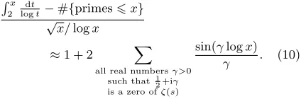
To focus on the overcount in Gauss’s guesstimate for the number of primes up tox, we use the following approximation, which can be deduced from (7) if, and only if, the Riemann hypothesis is true:
x 2
dt
logt−#{primesx} √x/logx
≈1 + 2
all real numbersγ>0 such that 1
2+iγ
is a zero ofζ(s)
sin(γlogx)
γ . (10)
The right-hand side here is the overcount in Gauss’s prediction for the number of primes up tox, divided by something that grows like√x. When we looked at the table of primes it seemed that this quantity should be roughly constant. However, that is not quite true as we see upon examining the right-hand side. The first term on the right-hand side, the “1”, corresponds to the contribution of the squares of the primes in (7). The subsequent terms correspond to the terms involv-ing the zeros ofζ(s) in (7); these terms have denomi-natorγ so the most significant terms in this sum are those with the smallest values of γ. Moreover, each of these terms is a sine wave, which oscillates, half the time positive and half the time negative. Having the “logx” in there means that these oscillations hap-pen slowly (which is why we hardly notice them in the table above), but they do happen, and indeed the quantity in (10) does eventually get negative. No one has yet determined a value ofxfor which this is neg-ative (that is, a value of x for which there are more thanx
2(1/logt) dtprimes up tox), though our best
guess is that the first time this happens is for
x≈1.398×10316.
How does one arrive at such a guess given that the table of primes extends only up to 1022? One begins by using the first thousand terms of the right-hand side of (10) to approximate the left-hand side; wherever it looks as though it could be negative, one approximates with more terms, maybe a million, until one becomes pretty certain that the value is indeed negative.
It is not uncommon to try to understand a given function better by representing it as a sum of sines and cosines like this; indeed this is how one studies the harmonics in music and (10) becomes quite compelling from this perspective. Some experts suggest that (10) tells us that “the primes have music in them” and thus makes the Riemann hypothesis believable, even desirable.
To prove unconditionally that
#{primesx} ∼
x
2
dt logt,
the so-called “prime number theorem,” we can take the same approach as above but, since we are not ask-ing for such a strong approximation to the number of primes up tox, we need to show only that the zeros near to the line Re(s) = 1 do not contribute much to the formula (7). By the end of the nineteenth cen-tury this task had been reduced to showing that there are no zeros actuallyon the line Re(s) = 1: this was eventually established byde la Vall´ee Poussinand Hadamardin 1896.
Subsequent research has provided wider and wider subregions of the critical strip without zeros of ζ(s) (and thus improved approximations to the number of primes up to x), without coming anywhere near to proving the Riemann hypothesis. This remains as an outstanding open problem of mathematics.
analysis—in fact, their argument is a complicated one. Of course their proof must somehow show that there is no zero on the line Re(s) = 1, and indeed their com-binatorics cunningly masks a subtle complex analysis proof beneath the surface (read Ingham’s discussion (1949) for a careful examination of the argument).
4 Primes in Arithmetic Progressions
After giving good estimates for the number of primes up to x, which from now on we shall denote byπ(x), we might ask for the number of such primes that are congruent to a mod q. (Modular arithmetic is discussed in Part III.) Let us write π(x;q, a) for this quantity. To start with, note that there is only one prime congruent to 2 mod 4, and indeed there can be no more than one prime in any arithmetic a, a+q, a+ 2q, . . . if a and q have a common fac-tor greater than 1. Let φ(q) denote the number of integers a, 1 a q, such that (a, q) = 1. (The notation (a, q) stands for the highest common factor ofaandq.) Then all but a small finite number of the infinitely many primes belong to the φ(q) arithmetic progressions a, a+q, a+ 2q, . . . with 1a < q and (a, q) = 1. Calculation reveals that the primes seem to be pretty evenly split between these φ(q) arithmetic progressions, so we might guess that in the limit the proportion of primes in each of them is 1/φ(q). That is, whenever (a, q) = 1, we might conjecture that, as x→ ∞,
π(x;q, a)∼π(x)φ(q). (11)
It is far from obvious even that the number of primes congruent toamodqis infinite. This is a famous the-orem of Dirichlet. To begin to consider such ques-tions we need a systematic way to identify integers n that are congruent toamodq, and this Dirichlet pro-vided by introducing a class of functions now known as(Dirichlet) characters. Formally, acharactermodq is a function χfromZ toCwith the following three properties (in ascending order of interest):
(i) χ(n) = 0 whenevernandqhave a common factor greater than 1;
(ii) χisperiodicmodq—that is,χ(n+q) =χ(n) for every integern;
(iii) χis multiplicative—that is, χ(mn) = χ(m)χ(n) for any two integersmandn.
An easy but important example of a character modq is theprincipal characterχq, which takes the value 1 if
(n, q) = 1 and 0 otherwise. Ifqis prime, then another important example is theLegendre symbol (·/q): one sets (n/q) to be 0 ifn is a multiple of q, 1 if n is a quadratic residue mod q, and −1 if n is a quadratic nonresidue modq. (An integernis called aquadratic residue mod q if n is congruent mod q to a perfect square.) Ifq is composite, then a function known as the Legendre–Jacobi symbol (·/q), which generalizes the Legendre symbol, is also a character. This too is an important example that helps us, in a slightly less direct way, to recognize squares modq.
These characters are all real-valued, which is the exception rather than the rule. Here is an example of a genuinely complex-valued character in the case q = 5. Set χ(n) to be 0 ifn ≡ 0 (mod 5), i if n ≡
2, −1 if n ≡ 4, −i if n ≡ 3, and 1 if n ≡ 1. To see that this is a character, note that the powers of 2 mod 5 are 2,4,3,1,2,4,3,1, . . ., while the powers of i are i,−1,−i,1,i,−1,−i,1, . . ..
It can be shown that there are precisely φ(q) dis-tinct characters modq. Their usefulness to us comes from the properties above, together with the following formula, in which the sum is over all characters modq and ¯χ(a) denotes the complex conjugate ofχ(a):
1 φ(q)
χ
¯
χ(a)χ(n) =
1 ifn≡a(modq), 0 otherwise.
What is this formula doing for us? Well, understanding the set of integers congruent toamodqis equivalent to understanding the function that takes the value 1 if n≡a (modq) and 0 otherwise. This function appears on the right-hand side of the formula. However, it is not a particularly nice function to deal with, so we write it as a linear combination of characters, which are much nicer functions because they are multiplica-tive. The coefficient associated with the character χ in this linear combination is the number ¯χ(a)/φ(q).
From the formula, it follows that
pprime, m1 pmx pm≡a (modq)
logp
= 1 φ(q)
χ (modq)
¯
χ(a)
pprime, m1 pmx
The sum on the left-hand side is a natural adaptation of the sum we considered earlier when we were count-ing all primes. And we can estimate it if we can get good estimates for each of the sums
pprime, m1 pmx
χ(pm) logp.
We approach these sums much as we did before, obtaining an explicit formula, analogous to (7), (10), now in terms of the zeros of theDirichletL-function:
L(s, χ) :=
n1
χ(n) ns .
This function turns out to have properties closely analogous to the main properties ofζ(s). In particular, it is here that the multiplicativity ofχis all-important, since it gives us a formula similar to (1):
n1
χ(n) ns =
pprime
1−χ(p)ps
−1
. (12)
That is,L(s, χ) has anEuler product. We also believe the “generalized Riemann hypothesis” that all zerosρ of L(ρ, χ) = 0 in the critical strip satisfy Re(ρ) = 12. This would imply that the number of primes up tox that are congruent toamodq can be estimated as
π(x;q, a) =π(x) φ(q) +O(
√
xlog2(qx)). (13)
Therefore, the generalized Riemann hypothesis implies the estimate we were hoping for (formula (11)), provided thatxis a little bigger thanq2.
In what range can we prove (11) unconditionally— that is, without the help of the generalized Riemann hypothesis? Although we can more or less translate the proof of the prime number theorem over into this new setting, we find that it gives (11) only whenxis very large. In fact,xhas to be bigger than an expo-nential in a power ofq—which is a lot bigger than the “xis a little larger thanq2” that we obtained from the
generalized Riemann hypothesis. We see a new type of problem emerging here, in which we are asking for a good starting point for the range ofxfor which we obtain good estimates, as a function of the modulus q; this does not have an analogy in our exploration of the prime number theorem. By the way, even though this bound “xis a little larger than q2” is far out of reach of current methods, it still does not seem to be the best answer; calculations reveal that (11) seems
to hold whenxis just a little bigger thanq. So even the Riemann hypothesis and its generalizations are not powerful enough to tell us the precise behaviour of the distribution of primes.
Throughout the twentieth century much thought was put in to bounding the number of zeros of Dirich-let L-functions near to the 1-line. It turns out that one can make enormous improvements in the range of xfor which (11) holds (to “halfway between polyno-mial inq and exponential in q”) provided there are noSiegel zeros. These putative zeros β ofL(s,(·/q)) would be real numbers withβ >1−c/√q; they can be shown to be extremely rare if they exist at all.
That Siegel zeros are rare is a consequence of the Deuring–Heilbronn phenomenon: that zeros of L-functions repel each other, rather like similarly charged particles. (This phenomenon is akin to the fact that different algebraic numbers repel one another, part of the basis of the subject of Diophantine approximation.)
How big is the smallest prime congruent toamodq when (a, q) = 1? Despite the possibility of the exis-tence of Siegel zeros, one can prove that there is always such a prime less thanq5.5 if q is sufficiently large.
Obtaining a result of this type is not difficult when there are no Siegel zeros. If there are Siegel zeros, then we go back to the explicit formula, which is similar to (7) but now concerns zeros ofL(s, χ). Ifβ is a Siegel zero, then it turns out that in the explicit formula there are now two obviously large terms:x/φ(q) and
−(a/q)xβ/βφ(q). When (a/q) = 1 it appears that they
might almost cancel (sinceβis close to 1), but with more care we obtain
x−(a/q)x
β
β = (x−x
β) +xβ1 −β1
∼x(1−β) logx.
This is a smaller main term than before, but it is not too hard to show that it is bigger than the contri-butions of all of the other zeros combined, because the Deuring–Heilbronn phenomenon implies that the Siegel zero repels those zeros, forcing them to be far to the left. When (a/q) =−1, the same two terms tell us that if (1−β) logx is small, then there are twice as many primes as we would expect up toxthat are congruent toamodq.
number formula states that L(1,(·/q)) = πh−q/√q
for q > 6, where h−q is the class number of the
field Q(√−q) (for more on this topic, see Section 7 of Algebraic Numbers). A class number is always a positive integer, so this result immediately implies thatL(1,(·/q))π/√q. Another consequence is that h−q is small if and only if L(1,(·/q)) is small. The
reason this gives us information about Siegel zeros is that one can show that the derivative L′(σ,(·/q)) is
positive (and not too small) for real numbersσclose to 1. This implies thatL(1,(·/q)) is small if and only ifL(s,(·/q)) has a real zero close to 1, that is, a Siegel zero β. When h−q = 1, the link is more direct: it
can be shown that the Siegel zeroβis approximately 1−6/(π√q). (There are also more complicated formu-las for larger values ofh−q.)
These connections show that getting good lower bounds onh−q is equivalent to getting good bounds
on the possible range for Siegel zeros. Siegel showed that for any ε > 0 there exists a constant cε > 0
such that L(1,(·/q))cεq−ε. His proof was
unsatis-factory because by its very nature one cannot give an explicit value for cε. Why not? Well, the proof
comes in two parts. The first assumes the generalized Riemann hypothesis, in which case an explicit bound follows easily. The second obtains a lower bound in terms of the first counterexample to the generalized Riemann hypothesis. So if the generalized Riemann hypothesis is true but remains unproved, then Siegel’s proof cannot be exploited to give explicit bounds. This dichotomy, between what can be proved with an explicit constant and what cannot be, is seen far and wide in analytic number theory—and when it appears it usually stems from an application of Siegel’s result, and especially its consequences for the range in which the estimate (11) is valid.
A polynomial with integer coefficients cannot always take on prime values when we substitute in an integer. To see this, note that if p divides f(m) then p also divides f(m+p), f(m+ 2p), . . .. How-ever, there are some prime-rich polynomials, a famous example being the polynomial x2+x+ 41, which is
prime for x = 0,1,2, . . . ,39. There are almost cer-tainly quadratic polynomials that take on more con-secutive prime values, though their coefficients would have to be very large. If we ask the more restricted question of when the polynomial x2+x+pis prime for x = 0,1,2, . . . , p−2, then the answer, given by
Rabinowitch, is rather surprising: it happens if and only ifh−q= 1, whereq= 4p−1. Gauss did extensive
calculations of class numbers and predicted that there are just nine values ofq withh−q= 1, the largest of
which is 163 = 4×41−1. Using the Deuring–Heilbronn phenomenon researchers showed, in the 1930s, that there is at most one q with h−q = 1 that is not
already on Gauss’s list; but as usual with such meth-ods, one could not give a bound on the size of the putative extra counterexample. It was not until the 1960s that Baker and Stark proved that there was no tenthq, both proofs involving techniques far removed from those here (in fact Heegner gave what we now understand to have been a correct proof in the 1950s but he was so far ahead of his time that it was difficult for mathematicians to appreciate his arguments and to believe that all of the details were correct). In the 1980s Goldfeld, Gross, and Zagier gave the best result to date, showing thath−q 77001 logqthis time using
the Deuring–Heilbronn phenomenon with the zeros of yet another type of L-function to repel the zeros of L(s,(·/q)).
This idea that primes are well distributed in arith-metic progressions except for a few rare moduli was exploited by Bombieri and Vinogradov to prove that (11) holds “almost always” when x is a little big-ger than q2 (that is, in the same range that we get “always” from the generalized Riemann hypothesis). More precisely, for given large x we have that (11) holds for “almost all”qless than√x/(logx)2 and for
alla such that (a, q) = 1. “Almost all” means that, out of allq less than√x/(logx)2, the proportion for
which (11) does not hold for everya with (a, q) = 1 tends to 0 asx→ ∞. Thus, the possibility is not ruled out that there are infinitely many counterexamples. However, since this would contradict the generalized Riemann hypothesis, we do not believe that it is so.
TheBarban–Davenport–Halberstam theoremgives a weaker result, but it is valid for the whole feasible range: for any given large x, the estimate (11) holds for “almost all” pairsqandasuch thatqx/(logx)2 and (a, q) = 1.
5 Primes in Short Intervals
inter-pret his statement by considering the number of primes in short intervals at around x. If we believe Gauss, then we might expect the number of primes between x and x+y to be about y/logx. That is, in terms of the prime-counting function π, we might expect that
π(x+y)−π(x)∼logyx (14)
for |y| x/2. However, we have to be a little care-ful about the range fory. For example, ify=1
2logx,
then we certainly cannot expect to have half a prime in each interval. Obviously we needyto be large enough that the prediction can be interpreted in a way that makes sense; indeed, the Gauss–Cram´er model sug-gests that (14) should hold when|y|is a little bigger than (logx)2.
If we attempt to prove (14) using the same methods we used in the proof of the prime number theorem, we find ourselves bounding differences betweenρth pow-ers as follows:
(x+y)ρ−xρ ρ
=
x+y
x
tρ−1dt
x+y
x
tRe(ρ)−1dty(x+y)Re(ρ)−1.
With bounds on the density of zeros of ζ(s) well to the right of 1
2, it has been shown that (14) holds fory
a little bigger thanx7/12; but there is little hope, even
assuming the Riemann hypothesis, that such methods will lead to a proof of (14) for intervals of length √x or less.
In 1949 Selberg showed that (14) is true for “almost all”xwhen|y|is a little bigger than (logx)2, assum-ing the Riemann hypothesis. Once again, “almost all” means 100%, rather than “all,” and it is feasible that there are infinitely many counterexamples, though at that time it seemed highly unlikely. It therefore came as a surprise when Maier showed, in 1984, that, for any fixedA >0, the estimate (14) fails for infinitely many integersx, withy= (logx)A. His ingenious proof rests
on showing that the small primes do not always have as many multiples in an interval as one might expect. Let p1 = 2 < p2 = 3 < · · · be the sequence of
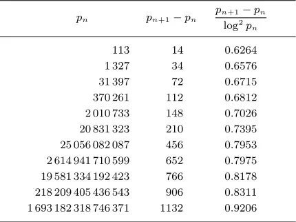
primes. We are now interested in the size of the gaps pn+1−pnbetween consecutive primes. Since there are
aboutx/logxprimes up tox, the average difference is logx and we might ask how often the difference between consecutive primes is about average, whether
Table 2 The largest known gaps between primes.
pn pn+1−pn
pn+1−pn
log2
pn
113 14 0.6264
1 327 34 0.6576
31 397 72 0.6715
370 261 112 0.6812 2 010 733 148 0.7026 20 831 323 210 0.7395 25 056 082 087 456 0.7953 2 614 941 710 599 652 0.7975 19 581 334 192 423 766 0.8178 218 209 405 436 543 906 0.8311 1 693 182 318 746 371 1132 0.9206
the differences can get really small, and whether the differences can get really large. The Gauss–Cram´er model suggests that the proportion ofnfor which the gap between consecutive primes is more thanλtimes the average, that ispn+1−pn> λlogpn, is
approxi-mately e−λ; and, similarly, the proportion of intervals [x, x+λlogx] containing exactlykprimes is approx-imately e−λλk/k!, a suggestion which, as we shall
see, is supported by other considerations. By looking at the tail of this distribution, Cram´er conjectured that lim supn→∞(pn+1−pn)/(logpn)2= 1, and the
divis-ibility by small primes, one is led to conjecture that lim supn→∞(pn+1−pn)/(logpn)2 is greater than 98.
Finding large gaps between primes is equivalent to finding long sequences of composite numbers. How about trying to do this explicitly? For example, we know that n! +jis composite for 2j n, as it is divisible by j. Therefore we have a gap of length at leastnbetween consecutive primes, the first of which is the largest prime less than or equal ton! + 1. How-ever, this observation is not especially helpful, since the average gap between primes aroundn! is log(n!), which is approximately equal to nlogn, whereas we are looking for gaps that arelarger than the average. However, it is possible to generalize this argument and show that there are indeed long sequences of consec-utive integers, each with a small prime factor. In the 1930s, Erd˝os reformulated the question as follows. Fix a positive integer z, and for each primepz choose an integerapin such a way that, for as large an
inte-geryas possible, every positive integernysatisfies at least one of the congruencesn≡ap (modp). Now
letX be the product of all the primes up toz (which means, by the prime number theorem, that logX is aboutz), and letxbe the integer betweenX and 2X such that x ≡ −ap (modp) for every p z. (This
integer exists, by theChinese remainder theorem.) If mis an integer betweenx+1 andx+y, thenm−xis a positive integer less thany, som−x≡ap (modp) for
some prime pz. Sincex≡ −ap (modp), it follows
that m is divisible by p. Thus, all the integers from x+ 1 tox+yare composite. Using this basic idea, it can be shown that there are infinitely many primespn
for whichpn+1−pnis about (logpn)(log logpn), which
is significantly larger than the average but nowhere close to Cram´er’s conjecture.
6 Gaps between Primes that are Smaller than the Average
We have just seen how to show that there are infinitely many pairs of consecutive primes whose difference is much bigger than the average: that is lim supn→∞(pn+1−pn)/(logpn) =∞. We would now
like to show that there are infinitely many pairs of con-secutive primes whose difference is much smaller than the average: that is lim infn→∞(pn+1−pn)/(logpn) =
0. Of course, it is believed that there are infinitely
many pairs of primes that differ by 2, but this ques-tion seems intractable for now.
Until recently researchers had very little success with the question of small gaps; the best result before 2000 was that there are infinitely many gaps of size less than one-quarter of the aver-age. However, a recent method of Goldston, Pintz, and Yildirim, which counts primes in short inter-vals with simple weighting functions, proves that lim infn→∞(pn+1−pn)/(logpn) = 0, and even that
there are infinitely many pairs of consecutive primes with difference no larger than about √logpn. Their
proof, rather surprisingly, rests on estimates for primes in arithmetic progressions; in particular, that (11) holds for almost allqup to√x(as discussed earlier). Moreover, they obtain a conditional result of the fol-lowing kind: if in fact (11) holds for almost allqup to a little larger than√x, then it follows that there exists an integer B such that pn+1−pn B for infinitely
many primespn.
7 Very Small Gaps between Primes
There appear to be many pairs of primes that differ by two, like 3 and 5, 5 and 7,. . ., the so-calledtwin primes, though no one has yet proved that there are infinitely many. In fact, for every even integer 2kthere seem to be many pairs of primes that differ by 2k, but again no one has yet proved that there are infinitely many. This is one of the outstanding problems in the subject.
In a similar vein is Goldbach conjecture’s from the 1760s: is it true that every even integer greater than 2 is the sum of two primes? This is still an open ques-tion, and indeed a publisher recently offered a million dollars for its solution. We know it is true for almost all integers, and it has been computer tested for every even integer up to 4×10¹⁴. The most famous result on this question is due to Jing-Run Chen (1966) who showed that every even integer can be written as the sum of a prime and a second integer that hasat most two prime factors (that is, it could be a prime or an “almost-prime”).
call the “Goldbach conjecture.” In the 1920s Vino-gradov showed that every sufficiently large odd inte-ger can be written as the sum of three primes (and thus every sufficiently large even integer can be writ-ten as the sum of four primes). We actually believe that every odd integer greater than 5 is the sum of three primes but the known proofs only work once the numbers involved are large enough. In this case we can be explicit about “sufficiently large”—at the moment the proof needs them to be at least e5700, but it is
rumored that this may soon be substantially reduced, perhaps even to 7.
To guess at the precise number of prime pairs q, q+ 2 with q x we proceed as follows. If we do not consider divisibility by the small primes, then the Gauss–Cram´er model suggests that a random integer up toxis prime with probability roughly 1/logx, so we might expect x/(logx)2 prime pairs q, q+ 2 up
to x. However, we do have to account for the small primes, as theq,q+ 1 example shows, so let us con-sider 2-divisibility. The proportion of random pairs of integers that are both odd is 14, whereas the propor-tion of randomq such thatq andq+ 2 are both odd is 1
2. Thus we should adjust our guessx/(logx) 2 by a
factor (1 2)/(
1
4) = 2. Similarly, the proportion of
ran-dom pairs of integers that are both not divisible by 3 (or indeed by any given odd prime p) is (2
3) 2 (and
(1−1/p)2, respectively), whereas the proportion of randomqsuch thatqandq+ 2 are both not divisible by 3 (or by primep) is 1
3 (and (1−2/p), respectively).
Adjusting our formula for each primepwe end up with the prediction
#{qx:qandq+ 2 both prime}
∼2
pan odd prime
(1−2/p) (1−1/p)2
x (logx)2.
This is known as the “asymptotic twin-prime conjec-ture.” Despite its plausibility there do not seem to be any practical ideas around for turning the heuris-tic argument above into something rigorous. The one good unconditional result known is that the number of twin primes less than or equal to xis never more than four times the quantity we have just predicted. One can make a more precise prediction replacing x/(logx)2 by x
2(1/(logt)
2) dt, and then we expect
that the difference between the two sides is no more thanc√xfor some constantc >0, a guesstimate that is well supported by computational evidence.
A similar method allows us to make predictions for the number of primes in any polynomial-type patterns. Letf1(t), f2(t), . . . , fk(t)∈Z[t] be distinct irreducible
polynomials of degree greater than or equal to 1 with positive leading coefficient, and defineω(p) to be the number of integers n (modp) for which p divides f1(n)f2(n)· · ·fk(n). (In the case of twin primes above
we havef1(t) = t,f2(t) =t+ 2 with ω(2) = 1 and
ω(p) = 2 for all odd primes p.) If ω(p) = p then p always divides at least one of the polynomial values, so they can be simultaneously prime just finitely often (an example of this is whenf1(t) =t,f2(t) = t+ 1,
in which caseω(2) = 2). Otherwise we have an admis-sible set of polynomials for which we predict that the number of integersn less thanxfor which all of f1(n), f2(n), . . . , fk(n) are prime is about
pprime
(1−ωf(p)/p)
(1−1/p)k
×log x
|f1(x)|log|f2(x)| · · ·log|fk(x)|
(15)
once x is sufficiently large. One can use a similar heuristic to make predictions in Goldbach’s conjec-ture, that is, for the number of pairs of primesp,qfor whichp+q= 2N. Again, these predictions are very well matched by the computational evidence.
There are just a few cases of conjecture (15) that have been proved. Modifications of the proof of the prime number theorem give such a result for admis-sible polynomials qt+a (in other words, for primes in arithmetic progressions) and for admissible at2+
btu+cu2∈Z[t, u] (as well as some other polynomials
in two variables of degree two). It is also known for a certain type of polynomial innvariables of degreen (the admissible “norm-forms”).
There was little improvement on this situation dur-ing the twentieth century until quite recently, when, by very different methods, Friedlander and Iwaniec broke through this stalemate showing such a result for the polynomialt2+u4, and then Heath-Brown did so for any admissible homogenous polynomial in two variables of degree three.
hard at work attempting to show that the number of four-term arithmetic progressions of primes is indeed well approximated by (15). They are also extending their results to other families of polynomials.
8 Gaps between Primes Revisited
In the 1970s Gallagher deduced from the conjectured prediction (15) (withfj(t) =t+aj) that the
propor-tion of intervals [x, x+λlogx] which contain exactly k primes is close to e−λλk/k! (as was also deduced,
in Section 5 above, from the Gauss–Cram´er heuris-tics). This has recently been extended to support the prediction that, as we vary x from X to 2X, the number of primes in the interval [x, x+y] is normally distributed with meanx+y
x (1/logt) dtand
variance (1−δ)y/logx, where δ is some constant strictly between 0 and 1 and we takeyto bexδ.
Wheny >√xthe Riemann zeta function supplies information on the distribution of primes in intervals [x, x+y) via the explicit formula (7). Indeed when we compute the “variance”
1 X
2X
X
pprime, x<px+y
logp−y 2
dx
using the explicit formula we obtain a sum of terms of the form 2X
X x
i(γj−γk)dx. Here we are assuming the
Riemann hypothesis and writing the zeros of ζ(s) as 1/2±iγn with 0< γ1 < γ2<· · ·. This sum is
domi-nated by the terms corresponding to those pairsγj,γk
for which|γj−γk|is small (in which case there is
lit-tle cancellation in the integral). Therefore, in order to understand the variance for the distribution of primes in short intervals we need to understand the distri-bution of the zeros ofζ(s) in short intervals. In 1973 Montgomery investigated this and suggested that the proportion of pairs of zeros ofζ(s) whose difference is less thanαtimes the average gap between consecutive zeros is given by the integral
α
0
1−
sinπθ
πθ 2
dθ, (16)
and he proved an equivalent form of this in a limited range. If the zeros were placed “randomly,” then (16) would be replaced by α. In fact (16) is about 19α3 for small α, which is far smaller thanα. This means that there are far fewer pairs of zeros of ζ(s) that
are close together than one might expect, which we express informally by saying that the zeros of ζ(s) repelone another.
In a now-famous conversation that took place at the Institute for Advanced Study in Princeton, Mont-gomery mentioned his ideas to the physicist Freeman Dyson. Dyson immediately recognized (16) as a func-tion that comes up in modelling energy levels in quan-tum chaos. Believing that this was unlikely to be a coincidence, he suggested that the zeros of the Rie-mann zeta function are distributed, in all aspects, like energy levels, which are in turn modelled on the distribution of eigenvalues of random Hermitian matrices. There is now substantial computational and theoretical evidence that Dyson’s suggestion is correct and can be extended to DirichletL-functions, as well as other types ofL-functions, and even to other statistics aboutL-functions.
One note of caution. Few of the conjectured con-sequences of this new “random matrix theory” have been unconditionally proved, or seem likely to be in the foreseeable future. It simply provides a tool to make predictions where that was too difficult to do before. However, there is at least one key question about which we still cannot make a well-substantiated prediction: how big doesζ(s) get on the 1
2-line? One
can show that log|ζ(1
2+ it)| gets larger than √
logT for values oft close toT, and that it gets no larger than logT. However, it is unclear, even if we do not insist on a rigorous proof, whether the true maximal order is nearer the upper or lower bound.
9 Sieve Methods
Almost all of our discussion so far has been about developments of Riemann’s approach to counting primes. This approach is very delicate and not as adaptable as one might wish to many natural ques-tions (such as countingk-tuples of primesn+a1, n+
a2, . . . , n+ak). However, one can go back to sieve
it is the case that neithernnorn+ 2 has a prime fac-tor less thany. If we tookyto be (2N)1/2, then this method would exactly count the twin primes, but it seems to be far too difficult to implement. But it turns out that if instead we take y to be a small power of N, then the calculations become much easier and there are ways of obtaining good bounds. (However, these bounds become less accurate as the power gets closer to 1
2.)
In the 1920s Brun showed how to make the prin-ciple of inclusion–exclusion into a useful tool in this type of question. This principle is best exhibited when counting the number of integersnin a setSthat are coprime to given integerm. We begin with the num-ber of integers inS, which is obviously more than the quantity we seek. Next, we subtract, for each prime p dividing m, the number of integers in S that are divisible byp. Ifn∈S is divisible by exactlyrprime factors of m, then we have counted 1 +r×(−1) for the contribution ofnso far, which is less than or equal to 0, and less than 0 forr2; whereas we wanted to count 0 when r 2 (since n is not coprime to m). Thus we obtain a number that is less than the quan-tity we seek. To compensate for that, we add back in the number of integers in S divisible by pq for each pair of primes p < q which divide m. We have now counted 1 +r×(−1) +r
2
×1 for the contribution ofn, which is greater than or equal to 0, and greater than 0 forr3. Similarly, we subtract the number of integers divisible bypqr, etc.
For each n ∈ S we end up counting (1−1)r for n, wherer is the number of distinct prime factors of (m, n). Expanding this sum with the binomial theorem we may reexpress this identity as follows. Letχm(n) =
1 if (n, m) = 1 and 0 otherwise. Then
χm(n) =
d|(m,n)
µ(d),
where µ(m), the M¨obius function, equals 0 if m is divisible by the square of a prime and equals (−1)ω(m)
otherwise, whereω(m) is the number of distinct prime factors ofm.
The inclusion-exclusion inequalities just discussed may be obtained from
d|(m,n) ω(d)2k+1
µ(d)χm(n)
d|(m,n) ω(d)2k
µ(d),
which holds for anyk0, by summing over alln∈S.
The reason for using these abbreviated sums rather than the complete sum is that there are far fewer terms and thus, when one sums over values ofn, there will be far fewer rounding errors (remember that it was rounding errors that sank our attempt to estimate the number of primes up toxusing the sieve of Eratos-thenes). On the other hand, they have the disadvan-tage that they cannot possibly give the exact answer, since they are missing many appropriate terms. How-ever, with a judicious choice ofkthe missing terms do not contribute much to the complete sum and we get a good answer.
Minor variants work well for many questions. In the “combinatorial sieve” one selects whichdare part of the upper and lower bound sums, not by counting the total number of prime factors they contain but instead using other criteria, such as the numbers of prime fac-tors of d in each of several intervals. Using such a method Brun showed that there cannot be too many twin primesp,p+ 2; indeed that the sum of 1/p, over all primesp for whichp+ 2 is also prime, converges, in contrast with (3).
In the “Selberg upper bound sieve” one comes up with some numbers λd that are nonzero only when
dD (whereD is chosen to be not too large), with the property that
χm(n)
d|n
λd
2
for alln.
Summing over the appropriate n one then finds the optimal solution by minimizing the resulting quadratic form. Lower bounds can also be obtained out of Sel-berg’s methods. It was using such methods that Chen was able to prove there are infinitely many primesp for whichp+2 has at most two prime factors, and that Goldston, Pintz, and Yildirim were able to establish that there are sometimes short gaps between primes. It is also an essential ingredient in the work of Green and Tao. One can also get good upper bounds on the number of primes in arithmetic progressions and short intervals:
• there are never more than 2y/logyprimes in any interval of lengthy;
• there are never more than 2x/φ(q) log(x/q) primes up toxin an arithmetic progression modq.
x/q, respectively), not logxas expected, though this will only make a significant difference if the number of integers being considered is small. Otherwise these inequalities are bigger than the expected quantity by a factor of 2. Can this “2” be improved? It will be dif-ficult because we showed earlier that if there are Siegel zeros then we get twice as many primes as expected in certain arithmetic progressions. Therefore, if we can improve the “2” in these two formulas, then we can deduce that there are no Siegel zeros!
10 Smooth Numbers
An integer is y-smooth if all of its prime factors are less than or equal toy. A proportion 1−log 2 of the integers up toxare √x-smooth, and indeed, for any fixedu >1 there exists some number ρ(u)>0 such that ifx=yu, then a proportionρ(u) of the integers
up toxarey-smooth. This proportion does not seem to have any easy definition in general. For 1u2 we have ρ(u) = 1−logu, but for largeru it is best defined as
ρ(u) := 1 u
1
0
ρ(u−t) dt,
anintegral delay equation. Such an equation is typical when we give precise estimates for questions that arise in sieve theory.
Questions about the distribution of smooth num-bers arise frequently in the analysis of algorithms, and have consequently been the focus of a lot of recent research. (See computational number theoryfor an example of the use of smooth numbers.)
11 The Circle Method
Another method of analysis that plays a prominent role in this subject is the so-calledcircle method, which goes back toHardyand Littlewood. This method uses the fact that, for any integern,
1
0
e2iπntdt=
1 ifn= 0, 0 otherwise.
For example, if we wish to count the number, r(n), of solutions to the equation p+q =n with pand q
prime, we can express it as an integral as follows:
r(n) =
p,qn both prime
1
0
e2iπ(p+q−n)tdt
= 1
0
e−2iπnt
pprime, pn
e2iπpt 2
dt.
The first equality holds because the integrand is 0 when p+q = n and 1 otherwise, and the second is easy to check.
At first sight it looks more difficult to estimate the integral than it is to estimater(n) directly, but this is not the case. For instance, the prime number theo-rem for arithmetic progressions allows us to estimate P(t) :=
pne
2iπpt whentis a rationalℓ/mwithm
small. For in this case,
P
ℓ m
=
(a,m)=1
e2iπaℓ/m
pn, p≡a (modm)
1
≈
(a,m)=1
e2iπaℓ/mπ(n)
φ(m) =µ(m) π(n) φ(m).
Iftis sufficiently close toℓ/m, thenP(t) ≈P(ℓ/m); such values of t are called the major arcs and we believe that the integral over the major arcs gives, in total, a very good approximation tor(n); indeed we get something very close to the quantity one predicts from something like (15). Thus to prove the Goldbach conjecture we need to show that the contribution to the integral from the other values oft(that is, from theminor arcs) is small. In many problems one can successfully do this, but no one has yet succeeded in doing so for the Goldbach problem. Also useful is the “discrete analogue” of the above: using the identity
1 m
m−1
j=0
e2iπjn/mdt=
1 ifn≡0 (modm),
0 otherwise
(which holds for any given integer m 1), we have that
r(n) =
p,qn both prime
1 m
m−1
j=0
e2iπj(p+q−n)/m
=
m−1
j=0
e−2iπjn/mP(j/m)2
allows us to use properties of the multiplicative group modm.
Sums likeP(j/m) in the paragraph above, or more simple sums like
nNe 2iπnk/m
are called “exponen-tial sums.” They play a central role in many of the cal-culations one does in analytic number theory. There are several techniques for investigating them.
(1) It is easy to sum the geometric progression
nNe
2iπn/m. With higher-degree polynomials one
can often reduce to this case; for example, by writing n1−n2=hwe have
nN
e2iπn2/m
2
=
n1,n2N
e2iπ(n21−n22)/m
=
|h|N
e2iπh2/m
max{0,−h}<n2
min{N,N−h}
e4iπhn2/m,
and the inner sum is now a geometric progression.
(2) The work of Weil and Deligne, which gives very accurate results on the number of solutions to equa-tions mod p, is ideally suited to many applications in analytic number theory. For example, the “Kloost-erman sum”
a1a2···ak≡b(modp)e
2iπ(a1+a2+···+ak)/p, where the ai run over the integers mod p and
(b, q) = 1, appears naturally in many questions; Deligne showed that it has absolute value less than or equal to kp(k−1)/2, an extraordinary amount of can-cellation in this sum which has aboutpk−1summands,
each of absolute value 1.
(3) We discussed earlier the fact that the values ofζ(s) satisfy a symmetry about the line Re(s) = 1
2, given by
the “functional equation.” There are other functions (called “modular functions”) that also have symme-tries in the complex plane; typically the value of the function at s is related to the value of the function at (αs+β)/(γs+δ), for some integersα,β,γ,δ sat-isfying αδ−βγ= 1. Sometimes an exponential sum can be related to the value of a modular function, and subsequently to the value of that modular function at another point, using the symmetry of the function.
12 MoreL-Functions
There are many types ofL-functions beyond Dirichlet L-functions, some of which are well understood, some
not. The type that have received the most attention recently are a class ofL-functions that can be asso-ciated with elliptic curves (see p.??of Arithmetic Geometry). Anelliptic curveEis given by an equa-tion of the formy2=x3+ax+b, where the
discrimi-nant4a3+ 27b2is nonzero. The associatedL-function
L(E, s) is most easily described in terms of its Euler product:
L(E, s) =
p
1−ap
ps +
p p2s
−1
. (17)
Hereapis an integer which, for primespnot dividing
4a3+ 27b2, is defined to be p minus the number of
solutions (x, y) (modp) to the equationy2≡x3+ax+
b (modp). It can be shown that each|ap|is less than 2√p, so the Euler product above converges absolutely when Re(s)> 3
2. Therefore, (17) is a good definition
for these values of s. Can we now extend it to the whole of the complex plane, as we did forζ(s)? This is a very deep problem—the answer is yes; in fact, it is the celebrated theorem of Andrew Wiles that implied Fermat’s last theorem.
Another interesting question is to understand the distribution of values of ap/2√p as we range over
primes p. These all lie in the interval [−1,1]. One might expect them to be uniformly distributed in the interval, but in fact this is never the case. As discussed inalgebraic numbersone can writeap=αp+ ¯αp,
where|αp|=√p, andαpwas called the Weil number.
If we writeα =√pe±iθp, then a
p = 2√pcos(θp) for
some angle θp ∈ [0, π]. We can then think of θp as
belonging to the upper half of a circle. The surprise is that for almost all elliptic curves theθp are not
uni-formly distributed, which would mean the proportion in a certain arc would be proportional to the length of that arc. Rather, they are distributed in such a way that the proportion of them in any given arc is pro-portional to the area under that arc. This is a recent result of Richard Taylor.
The correct analogue of the Riemann hypothesis for L(E, s) turns out to be that all the nontrivial zeros lie on the line Re(s) = 1. This is believed to be true. Moreover, it is believed that they, like the zeros ofζ(s), are distributed according to the rules that govern the eigenvalues of randomly chosen matrices.