A fed back level-set method for moving
material–void interfaces
1B. Korena;∗, A.C.J. Venisb
a
CWI, P.O. Box 94079, 1090 GB Amsterdam, The Netherlands b
MacNeal-Schwendler (E.D.C.) B.V. Groningenweg 6, 2803 PV Gouda, The Netherlands
Abstract
This report is a feasibility study of a level-set method for the computation of moving material–void interfaces in an Eulerian formulation. The report briey introduces level-set methods and focuses on the development of such a method, that does not just accurately resolve the geometry of the interface, but also the physical quantities at and near the interface. Results are presented for illustrative model problems. As concerns its ability to improve the geometrical resolution of free boundaries, as expected, the level-set method performs excellently. Concerning the improvement of physical (all other than merely geometrical) free-boundary properties, the method performs very well for downstream-facing fronts and is promising for upstream-facing ones. c1999 Elsevier Science B.V. All rights reserved.
AMS classication:65M20; 65M99; 76M99; 76T05
Keywords:Free-boundary problems; Material–void interfaces; Discretization of convection equations; Level-set methods
1. Introduction
1.1. Problem denition
The subject of this paper is the investigation and further development of a numerical method which is promising for the computation of a special class of free-boundary problems: moving material interfaces, in application areas such as forging and sloshing. Particularly in the rst application area, the accuracy requirements imposed on the geometrical and physical resolution of the interface are very high. (With physical resolution we mean that of quantities such as velocity, density, stresses, etc.) In both applications, in general, proper use may be made of the property that at one side of the
∗Corresponding author. Tel.: +31.205924114; fax: +31. 205924199; e-mail: [email protected].
1This research was performed for MacNeal-Schwendler (E.D.C.) B.V., and was nancially supported by the Netherlands Ministry of Economic Aairs, through its programmeSenter.
interface, the material can be modeled as void. E.g., with steel and air at either side of the interface, the modeling of air as void is quite realistic. In the present paper, material–void interfaces will be considered only. For reasons of transparency, the numerical methods considered are not applied to real interface problems, but to clarifying model problems with known exact solutions.
1.2. Existing computational approaches
The existing computational approaches for free-boundary problems are Lagrangian, Eulerian or a combination of both: Arbitrary Lagrangian–Eulerian (ALE). In the Lagrangian approach, the grid is attached to the free boundary. As a consequence, the fronts resolved in this way are crisp. But they are not necessarily accurate; their location, even their topology, may be inaccurate. A known drawback of the Lagrangian approach is that it is not well-suited for the computation of bifurcating free boundaries. The Eulerian approach, in which the front moves through a grid which is xed in space, does not have this drawback, but — as is known — here the fronts are diused. The ALE technique attempts to avoid both drawbacks. In it, a grid is attached to the front, but it is remeshed in due time, after great distortions or bifurcations. In case of rapid great distortions or rapid bifurcations, frequent remeshing is needed, which is disadvantageous of course. In the present paper, we consider the pure Eulerian approach only.
In the pure Eulerian approach, since many years, some well-proven techniques exist for computing free-boundary ows. Known examples of these are the marker-and-cell (MAC) method (see, e.g., [7]) and the volume-of-uid (VOF) method (see, e.g., [4, 8]). Both methods have as a drawback that they may require intricate (subcell) bookkeeping to properly keep track of fronts. (In case of MAC, the subcell bookkeeping consists of investigating whether possibly occurring cavitating cells are either numerical or physical.) In principle, all this bookkeeping can be avoided in a more recent class of computing methods for free-boundary ows: the so-called level-set methods. A text book on level-set methods is [17], a classical journal paper is [15]. Since [15], many more journal papers have appeared on level-set methods, various of these directed towards uid-ow applications (see, e.g., [2, 3, 5, 6, 9, 13, 18, 20]). In all these papers, the interfaces considered are of material–material type. Material–void interfaces, the subject of this paper, seem to be novel.
1.3. Level-set methods
Because of their nonsmoothness, moving fronts cannot be captured suciently accurate on xed grids. No advantage can be taken of nice numerical accuracy properties, valid for smooth solutions only. As a natural x to this, in the level-set method, to the system of physical unknowns, a nonphysical unknown is added, which is smooth at the front: the level-set function. Furthermore, a nonphysical equation is added: a convection equation for the level-set function. E.g, to the Euler equations written in conservative variables, one may add the level-set function = (x; y; z; t);which is convected as — in principle — a passive scalar, by the likewise conservative equation
@( )
@t +
@(u )
@x +
@(v )
@y +
@(w )
This leads to the extended system
Note that in system (1.2), is a passive scalar indeed; there is no feedback of the convection of into that of mass, momentum or energy. If one is only interested in an accurate geometrical resolution of the interface, in principle, a feedback is not necessary. In case of a free-boundary computation of, e.g., two nonmixing gases at dierent densities, the standard Eulerian diculty to accurately resolve the geometry of the discontinuous gas interface may be directly alleviated by taking for the level-set function an initial solution which is smooth everywhere (so also at the initial gas interface) and which has a pre-dened and constant value at the interface, a value which exists at the interface only. Then it is clear that to accurately resolve the gas interface — instead of following the density jump – one can better keep track of this pre-dened interface value for — say f — because one can
take maximal advantage of the smoothness of . (For the density, the accuracy properties of most higher-order accurate discretizations break down at precisely the point of interest: the interface.) This easy possibility for creating smoothness at the interface (through a smooth, articial, passive scalar function) is a rst interesting property of the level-set method. Related to this, a second interesting property is that the interface location is neatly dened (viz., as the location where = f): With a
physical jump at the interface from, say, c= 1 to c= 0 (where c models, e.g., the material density), in case of a diused grid-representation of this jump, it is not immediately clear how to precisely dene the interface location. (Should one dene it as there where c=12 orc=h;withh the mesh size, or as whatever?) A third interesting property of the level-set technique is that the level-set function requires no new, specically tailored discretization method. The discretization method that one has in mind for the physical system, can be easily and consistently extended with the new conservation equation for . So, as opposed to uid markers or volume-of-uid fractions, the level-set function can be directly and consistently embedded in the existing, discrete system of physical equations. Related to this, a fourth advantage of level-set methods is that there is no diculty in extending the system of equations from 2-D to 3-D.
oers a possibility that seems to be new. A physically sound feedback of the level-set function may be incorporated into the real (physical) equations. In all level-set literature known to us, if there is a feedback of the level-set function into physics, it is restricted to material properties such as the ratio of specic heats (=( )) and the kinematic viscosity (=( )): In the present paper, the level-set function will be explicitly fed back into the computation of the physical ux function
f=f(c): I.e., in the discrete case, we extend this to f=f(c; ):
The contents of the paper is the following. In Section 2, we present two model problems to be considered throughout this paper and we present reference results for it. In Section 3, a standard level-set method is considered, one without feedback into the physical system. Simple shape-tracking results are presented for it. The level-set method with feedback is presented in Section 4, together with results for the two test cases. Concluding remarks are given in Section 5.
2. Test cases and reference results
2.1. Model problems and exact discrete solutions
In the model problems to be considered, the multi-dimensional convection of an interface is the issue. In here, as mentioned, we are not only interested in shape preservation. The problems are described by the 2-D, linear, unsteady convection equation
@c @t +u
@c @x +v
@c
@y = 0; (x; y)∈[−1;1]×[−1;1]; (2.1)
with as initial conditions:
c(x; y; t= 0) =
1; (x; y)∈(x−xc)2+ (y−yc)26(15)2; xc=yc=−12;
0 elsewhere; (2.2a)
and
c(x; y; t= 0) =
1; (x; y)∈[xc−15; yc−15]×[xc+15; yc+15]; xc=yc=−12;
0 elsewhere: (2.2b)
For the velocity eld, dened for positive c only (i.e., in the material only), we simply take
u=v= 1; (2.3)
and for the inlet boundary conditions we take
c(x=−1; y; t) =c(x; y=−1; t) = 0: (2.4) So, the problems describe the diagonal transport in a square domain, of successively a circular initial solution, (2.2a), and a square initial solution, (2.2b). Requested for both the circle and the square:
c(x; y; t= 1):The exact solutions are identical to the initial solutions (2.2a) and (2.2b), but now with
xc=yc=12: (For other initial values of xc and yc, this problem was already considered in [1].)
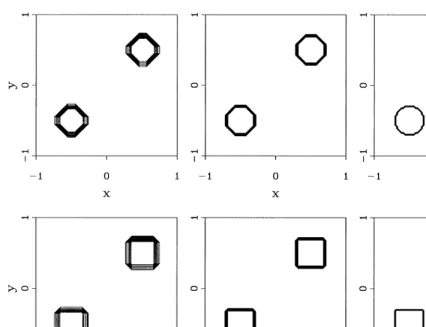
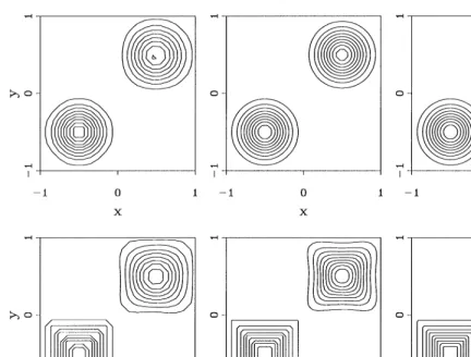
Both problems are solved on equidistant, cell-centered nite-volume grids with successively 20×20, 40×40 and 80×80 cells, so forhx=hy=h=101;201 and 401: Fig. 1 shows iso-line distributions of the
Fig. 1. Intial and nal exact discrete solutions for convection circle (up) and square (down), for from left to right:
h= 1 10;
1 20;
1 40.
2.2. Standard numerical method
The cell-centered nite-volume discretization of the integral form of (2.1) yields, on an equidistant grid with hx=hy=h; the semi-discrete equation
1
h
Z Z @c
@t dxdy+u(ci+1=2; j−ci−1=2; j) +v(ci; j+1=2−ci; j−1=2) = 0: (2.5)
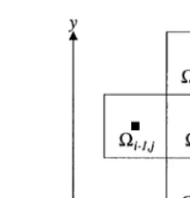
In here, the half-integer indices i− 1
2; j and i+ 1
2; j refer to the vertical cell faces @i−1=2; j and
@i+1=2; j, in between the cells i−1; j andi; j; and i; j and i+1; j, respectively (Figure 2). Likewise,
the indices i; j− 1
2 and i; j+ 1
2 refer to the horizontal cell faces @i; j−1=2 and @i; j+1=2, separating
Fig. 2. Cell-centered nite volume i; j with nearest neighbors.
We proceed by giving the standard numerical scheme for computing the cell-face uxes in the present two problems. At the vertical cell faces @i+1=2; j; i= 0;1; : : : ; n; j= 1;2; : : : ; n we apply
This limiter is a more accurate version of the =1
3-limiter presented in [11]. Concerning its TVD-properties, it can be directly seen that limiter (2.7) ts into Sweby’s TVD domain [19]:
06(r)6min(2r;2) for r¿0; (2.8a)
(r) = 0 for r60: (2.8b)
Concerning the accuracy properties of (2.7), while the=1
new = 1
3-limiter (2.7) also gives third-order accuracy in smooth extrema. To show these good accuracy properties, consider the 1-D model equation dc=dx = 0. The corresponding equation for nite volume i reads
ci+1=2−ci−1=2= 0; (2.9)
(The present in (2.6) has been omitted here; it is meant to avoid division by zero in practice, in the situation of a locally constant ow eld.) Let us rst consider the situation of a locally, monotonously increasing or decreasing solution and next that of a smooth extremum.
Locally monotonous solution. For this situation, through Taylor-series expansion aroundci, for ri+1=2 and ri−1=2 we nd
r= 1. Doing so, after further expansion around ci, from (2.9) and (2.10) it follows the modied
equation
So, to get third-order accuracy in monotonous ow regions, the limiter function (r) must satisfy
(1) = 1; (2.13a)
d(1) dr =
2
3: (2.13b)
Limiter (2.7) satises these requirements (as does the old limiter from [11]).
Smooth extremum. For a smooth extremum, through Taylor-series expansion aroundci, and through
the assumption that the extremum coincides with the cell center i (i.e., dci=dx= 0), we nd
ri−1=2=
and (2.10) we now get the modied equation
1
Limiter (2.7) satises these additional requirements. (The limiter from [11] does not.) The standard space discretization has been dened now.
Time integration. For the time integration we simply take the standard, four-stage Runge–Kutta scheme, which is fourth-order time-accurate for nonlinear problems. In all computational results to be presented hereafter, the time step is taken linearly proportional to the mesh size, and suciently small to ensure that time discretization errors are negligible with respect to space discretization errors. I.e., in all cases we take √u2+v2t=h61
2. According to [10], stability and monotonicity are guaranteed by these small time steps.
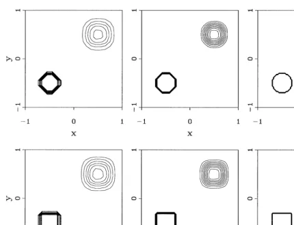
Reference results. In Fig. 3, as in Fig. 1, we give the iso-line distributions of the initial and nal solutions. (Iso-lines are given again at c= 0:1n; n= 1; : : : ;9:) In Table 1, some more quantitative information is given about these numerical solutions. In here, kck1 and kck∞ are the L1- and
L∞-norms of the solution errors. Due to the being discontinuous of both initial solutions, we observe
a rst-order accuracy behavior in kck1 and a zeroth-order behavior in kck∞.
3. Present level-set method
3.1. Principle
To explain the principle of the present level-set method — rst without feedback — for trans-parency reasons we consider the 1-D convection equation
@c @t +u
@c
Fig. 3. Initial and nal numerical solutions for convection circle (up) and square (down), through limited k=1 3-scheme, for from left to right:h= 1
10; 1 20;
1 40. Table 1
Numerical results for convection circle (up) and square (down), through limited =1
3-scheme Circle h= 1
10 h=
1
20 h=
1 40
kck1 3:2×10⁻² 1:7×10⁻² 9:7×10⁻³
kck∞ 5:7×10−
1 5:0×10−1 5:1×10⁻¹ Square h= 1
10 h=
1
20 h=
1 40
kck1 3:6×10⁻² 2:0×10−2 1:2×10⁻²
kck∞ 5:5×10−
1 6:2×10⁻¹ 6:4×10⁻¹
Denoting the level-set function again by , the extended equation reads
@q @t +u
@q
@x = 0; q=
c
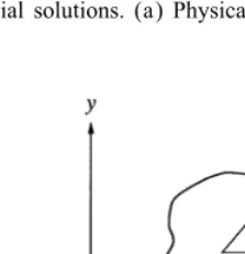
Fig. 4. Initial solutions. (a) Physical function; (b) level-set function.
Fig. 5. 2-D material–void interface.
Suppose that the initial solution c(x; t= 0) looks as in the sketch in Fig. 4a, i.e., with the interfaces at x= ±xf and with jumps from c= 1 to c= 0 over there. Then, for the corresponding initial
distribution of the level-set function, (x; t= 0); we propose the probability curve
(x; t= 0) = e−1=2(x=xf)2: (3.3)
A sketch of (3.3) is given in Fig. 4b. Note that (3.3) is innitely many times dierentiable at all points (including x= 0; a linear level-set function would not be dierentiable there). Higher-order accurate convection schemes can take full advantage of this dierentiability. Further note that the function has been chosen such that its inection points (its maximum slopes) coincide with the interfaces. (This gives the best posedness of the interface-detection problem.) In the level-set method, for the present 1-D model equation, a front is embedded in a 1-D function, while the front itself is a point-phenomenon only. This is typical for level-set methods: n-D physical fronts (n= 0;1 or 2) are embedded in (n+ 1)-D functions. We still remark that the choice (3.3) for the level-set function is rather arbitrary. Other functions, with equally good dierentiation properties, and interface values
f dierent from 1=√e; could have been chosen.
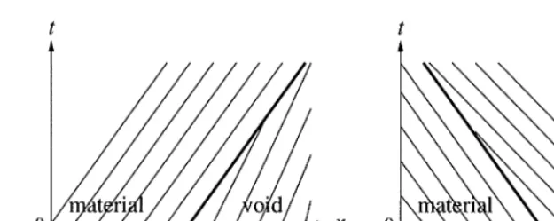
Fig. 6. Anti-convection for moving material–void interfaces. (a) Downstream-facing interface; (b) upstream-facing inter-face.
Next take as the initial level-set function
(r; ; t= 0) = e−1=2(r=rf)2; (3.4)
where rf=rf() is the radial distance from the point chosen to the material interface, for a given
angle ; ∈[0;2]. Doing so, we have f= 1=√e all over the interface. For many shapes, this
initialization works, also in 3-D, where it carries over in a spherical coordinate system.
3.2. Velocity eld
A subtle property of the convection of material–void interfaces is that the velocity eld is only dened in the material. Hence, for the convection of the level-set function in the void region, an articial velocity eld still has to be dened. The opportunity to make this choice, without being inhibited by physics, is a good chance in fact to improve the free boundary’s resolution. E.g., in the void region an articial velocity can be chosen which counteracts the eects of numerical diusion of the physical quantity c. For the 1-D convection equation (3.1), in the void region a velocity may be dened which looks as sketched in Fig. 6(a) and (b). So, for a downstream-facing front, u@ =@x ¡0; at the void side of the interface, a velocity may be chosen which is smaller than the velocity at the material side of the interface (Fig. 6(a)). This articial anti-convection implies converging characteristics and may thus lead to re-steepening of a diused front. To realize the steepening in case of an upstream-facing front, u@ =@x ¿0, the void velocity has to be taken greater than the material velocity (Fig. 6(b)).
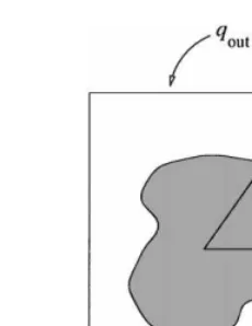
Fig. 7. Void region.
one can take the average velocity at the material interface. So, in 2-D, this elliptic velocity generator amounts to solving
3.3. Simple level-set results: shape tracking only
For the two test cases dened in Section 2.1, we can already present practically relevant level-set results now, viz. for the convection of the geometry. As the local origins of the r; -coordinate system introduced in Section 3.1, we simply take the centers of gravity of the initial circle and the initial square. For the initial function (r; ; t= 0) we take (3.4) and for its numerical convection scheme the non-limited =1
Fig. 8. Initial and nal numerical solutions for convection circular (up) and square (down) level-set function , through non-limited=1
3-scheme, for from left to right: h= 1 10;
1 20;
1 40:
with the radii r1=2; j(t); ri;1=2(t) and rf(t) exact for both the circular and the square shape. Applying
the identical time integration as in Section 2.2, the results depicted in Fig. 8 are obtained.
As in Tables 1 and 2, we give some more quantitative information about the numerical level-set solutions. As expected, higher-order accuracy isobtained here. For the circular shape,k k1 behaves almost third-order accurate. For the square solution, due to the nonsmoothness at the four corners, the accuracy behavior is less good: second-order almost, which is still better nevertheless than the orders of accuracy to be observed in Table 1.
Now the possibility also exists to compare the shape preservation properties of both approaches: the standard numerical (limited =13) approach from Section 2.2 and the present level-set approach. For additional comparison purposes, we also consider the corresponding, exact discrete solutions. For both the exact discrete solution and the solution obtained by the standard approach, the material interface is dened as the iso-line cf≡h (h being the mesh width). In the standard approach, as
Table 2
Numerical results for convection circular (up) and square (down) level-set function, through nonlimited =13 -scheme
Circular h= 1
10 h=
1
20 h=
1 40
k k1 9:5×10⁻³ 1:5×10⁻³ 1:9×10⁻⁴
k k∞ 1:6×10−
1 3:4×10⁻² 4:8×10⁻³ Square h= 1
10 h=
1
20 h=
1 40
k k1 1.4×10⁻² 4:4×10⁻³ 1:4×10⁻³
k k∞ 1:5×10−
1 9:3×10⁻² 5:0×10−2
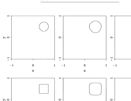
Fig. 9. Final shapes for circle (up) and square (down), for h= 1
40 and according to, from left to right: exact discrete solution c (iso-line c=cf=h), limited= 13-solutionc (iso-line c=cf=h) and nonlimited =13-solution (iso-line
= f=√1
level-set approach, this denition already exists: the iso-line f≡1=√e:For the 80×80-grid, in Fig. 9,
we present discrete shapes at t= 1, from left to right: (i) according to the exact discrete solution c, (ii) according to the limited =1
3 solution c and (iii) according to the nonlimited= 1
3 solution . (The iso-lines in the two most left graphs of Fig. 9 belong to the same solutions that have already been depicted in the two most right graphs of Fig. 1, and (likewise) the two middle graphs in Fig. 9 belong to the same solutions already depicted in the two most right graphs in Fig. 3.) For the circle, the dierence in quality between the standard numerical results and the level-set results is striking. Seen from Fig. 9, the shape preservation of the level-set circle is very good; numerical errors are very small. The depicted level-set circle is even more accurate than the plotted, exact discrete circle. The quality of the latter suers from the interface-denition problem. For the square, the level-set solution is less accurate than for the circle (because of the loss of one order of accuracy at the corners). Nevertheless, here as well, the level-set result is still much better than the standard numerical result in the middle graph.
4. Extended level-set results: Feedback with physics
The level-set results presented in the previous section are worthwhile. However, in practical appli-cations, shape preservation may not be the only goal. An accurate resolution of physical quantities at the interface may also be of interest. E.g., in a real uid dynamics problem, the velocity compo-nents at the interface are a particularly important issue, since they determine the motion of the free surface. Also, the density distribution along and near the interface may be of interest. Note that, so far, we do have obtained good shape preservation (the two right graphs in Fig. 9), but a physical quantity as density will still be diused at the interface (as demonstrated in the two middle graphs of Fig. 9). However, with the level-set function and equation added to a system of physical conservation laws, the useful knowledge to be extracted from the numerical solution of the level-set function does not need to be restricted to geometrical improvement of the free boundary only. Knowledge obtained from the level-set solution can also be fed back into the discretization of the physical equations. This feedback of the level-set function to physics is application-dependent and much eort may be put into it. Already for the present model for moving material–void interfaces, despite the model’s simplicity, it has appeared that dening the feedback is not straightforward; many possibilities exist. In [12], various feedback schemes are presented. Here, we present two such schemes. The model equation to be considered still is
@q @t +u
@q @x +v
@q
@y = 0; q=
c
; u=v= 1: (4.1)
4.1. First feedback
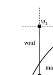
Fig. 10. Material–void interface cutting cell face.
cuts the cell face considered and where the corresponding cell-face value — say i+1=2; j — is less
than f. In such a case, the cell face should be left open. To realize this, we propose the following
scheme. First, we approximate the cell-vertex values 1 and 2 (Fig. 10). For the vertical cell faces
@i+1=2; j, i= 0;1; : : : ; n; j= 1;2; : : : ; n, these node values can be approximated by
( 1)i+1=2; j=
(
j= 1: i+1=2;1+12( i+1=2;1− i+1=2;2); else: 1
2( i+1=2; j−1+ i+1=2; j);
(4.2a)
( 2)i+1=2; j=
(
j=n: i+1=2; n+12( i+1=2; n− i+1=2; n−1); else: 1
2( i+1=2; j+ i+1=2; j+1);
(4.2b)
with i+1=2; j according to (3.6a). For the horizontal cell faces @i; j+1=2; i= 1;2; : : : ; n; j= 0;1; : : : ; n we have
( 1)i; j+1=2=
(
i= 1: 1; j+1=2+12( 1; j+1=2− 2; j+1=2); else: 12( i−1; j+1=2+ i; j+1=2);
(4.3a)
( 2)i; j+1=2=
(
i=n: n; j+1=2+12( n; j+1=2− n−1; j+1=2); else: 1
2( i; j+1=2+ i+1; j+1=2);
(4.3b)
with i; j+1=2 according to (3.6b). Then, at the vertical cell face @i+1=2; j, the rst feedback scheme
is
ci+1=2; j=
(((
1)i+1=2; j− f)(( 2)i+1=2; j− f)¡0: according to (2.6a) and (2.7);
else: max0; i+1=2; j−f
| i+1=2; j− f|
ci+1=2; j;
and at the horizontal cell face @i; j+1=2
ci; j+1=2=
(((
1)i; j+1=2− f)(( 2)i; j+1=2− f)¡0: according to (2:6b) and (2:7);
else: max0; i; j+1=2−f
| i; j+1=2− f|
ci; j+1=2;
(4.4b)
where ci+1=2; j and ci; j+1=2 in the right-hand sides are determined by (2.6) with limiter (2.7), and i+1=2; j and i; j+1=2 again by (3.6).
So, note that in (4.4), in fact, an extra limiting may be applied to the physical uxes, a limit-ing controlled by the level-set function. The level-set limitlimit-ing is binary; it either opens or closes cell faces. In the void region ( ¡ f) it may close cell faces. This obviously inhibits numerical
diusion into the void region. Note that to still preserve monotonicity, the original limiter (r) is still necessary. Since the binary limiter can have the values zero and one only, it cannot aect this monotonicity. Finally, note that the level-set limiter, with its ability to close cell faces, does not aect conservation; the basic nite-volume scheme remains unchanged. (What ows out of or into a cell across a face, remains to ow into or out of the cell neighboring that face.)
Numerical results obtained with this fed back scheme for each of the two test cases, are given in [12]. The results are not yet good; in the upstream void region, small amounts of mass may stagnate, they are pent up in cells with faces closed by the level-set limiter. The cause is clear; if in a cell
i; j; i−1=2; j; i+1=2; j; i; j−1=2 as well as i; j+1=2 are less than f and if the iso-line = f does not
cut any of the four cell faces @i−1=2; j; @i+1=2; j; @i; j−1=2 and @i; j+1=2; then all these four faces are closed, irrespective of the fact that there is still some mass in that cell (ci; j¿0).
4.2. Improved feedback
In improving the feedback, closure of cell faces will be done at the downstream sides of fronts only. In the upstream void region, an appropriate limiter will be applied: the superbee limiter [16]:
(r) =
0; r60;
2r; 0¡ r61
2; 1; 1
2¡ r61;
r; 1¡ r62;
2 else:
(4.5)
Because it is compressive, the superbee limiter will counteract diusion of the interface. Besides a front itself, its downstream and upstream sides can also be accurately distinguished by means of the level-set function. In 2-D, the downstream region is there where
(u; v)·3 ¡0: (4.6)
@
Now the complete ux formulae can be given. At the vertical cell faces we take:
i+1=2; j according to (3:6a);
And, similarly, at the horizontal cell faces:
i; j+1=2 according to (3.6b),
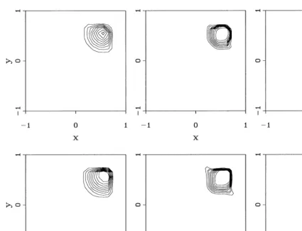
Fig. 11. Numerical solutionscfor convection circle (up) and square (down), through fed back level-set scheme, for from left to right: h= 1
10; 1 20;
1 40.
Table 3
Numerical results for convection circle and square, through fed back level-set scheme
Circle h= 101 h= 201 h= 401
kck1 2:0×10−2 1:1×10⁻² 5:4×10⁻³
kck∞ 5:4×10−
1 5:7×10⁻¹ 5:5×10⁻¹ Square h= 101 h=
1
20 h=
1 40
kck1 2:0×10−2 1:3×10⁻² 7:2×10⁻³
kck∞ 5:9×10⁻¹
6:0×10−1
Fig. 12. Curvilinear (left) and rectilinear (right) numerical solutionscfor convection downstream-facing interfaces, through standard (limited=1
3) scheme (h= 1 40).
In Section 4.1 of [5], Cocchi and Saurel present results for a test case comparable to the present diagonal convection of a square. (Cocchi and Saurel consider the diagonal convection of a square gas bubble.) In Fig. 24 of their paper, they show that they can accurately resolve a physical quantity (the density), not only at the downstream-facing part but also at the upstream-facing part of the interface. This dierence with our results can be explained from the dierence in methods; Cocchi and Saurel apply a sophisticated front-tracking method (with markers attached to the interface), whereas we apply a plain capturing method, without subcell resolution.
From the results in Fig. 11, it appears that the solution quality is particularly good at the downstream-facing interfaces. We illustrate this once more by means of the following simpli-cations of the two model problems. The equation and velocity to be considered are still the same, i.e., (2.1) and (2.3), respectively, but the initial solutions dier. Instead of (2.2a), rst we consider a downstream-facing curvilinear front only, viz.
c(x; y; t= 0) =
(
1; (x; y)∈(x−xc)2+ (y−yc)26(12)2; xc=yc=−1;
0 elsewhere, (4.9a)
and likewise, instead of (2.2b), the downstream-facing rectilinear front
c(x; y; t= 0) =
(
1; (x; y)∈[xc; yc]×[xc+12; yc+12]; xc=yc=−1;
0 elsewhere. (4.9b)
For both fronts, the corresponding boundary conditions are
c(x=−1; y; t) =
(
1; y6(yc+ 12) +vt;
0 elsewhere; (4.10a)
c(x; y=−1; t) =
(
1; x6(xc+ 12) +ut;
0 elsewhere. (4.10b)
In Fig. 12, the numerical solutions c at t= 1 are given, as obtained with the standard (i.e., the limited =1
Fig. 13. Curvilinear (left) and rectilinear (right) numerical solutionscfor convection downstream-facing interfaces, through fed back level-set scheme (h= 1
40).
approach are shown. Observation learns that the eect of closure of cell faces in the void region does not only lead to a thinning of the interface part diused into the void region, but also to a thinning of the part diused into the material.
5. Conclusions
For capturing free boundaries in an Eulerian formulation, the known advantages of level-set methods over most alternative Eulerian techniques are:
• level-set methods are smooth at physical discontinuities and, hence, allow us to maintain maximum numerical accuracy there,
• through the level-set function, the location of the discontinuity is clearly dened,
• the level-set function can be simply embedded in the system of physical equations and can be discretized collectively and consistently with these,
• there is no principal diculty in extending a level-set method from 2-D to 3-D. An additional advantage presented and worked out in this paper is that:
• the possibility exists to convect the level-set function as an active (instead of as a passive) scalar, i.e., to directly feed it back into the discretization of the physical equations (into the ux computations).
Acknowledgement
We thank the referees for their suggestions to improve this paper.
References
[1] C. Aalburg, Experiments in minimizing numerical diusion across a material boundary, M.Sc. Thesis, Department of Aerospace Engineering, University of Michigan, Ann Arbor, 1996. Also: http:==www.engin.umich.edu=research=
cfd=publications=publications.html.
[2] Y.C. Chang, T.Y. Hou, B. Merriman, S. Osher, A level set formulation of Eulerian interface capturing methods for incompressible uid ows, J. Comput. Phys. 124 (1996) 449 – 464.
[3] S. Chen, B. Merriman, S. Osher, P. Smereka, A simple level-set method for solving Stefan problems, J. Comput. Phys. 135 (1997) 8 – 29.
[4] A.J. Chorin, Flame advection and propagation algorithms, J. Comput. Phys. 35 (1980) 1 – 11.
[5] J.-P. Cocchi, R. Saurel, A Riemann problem based method for the resolution of compressible multimaterial ows, J. Comput. Phys. 137 (1997) 265 – 298.
[6] S.F. Davis, An interface tracking method for hyperbolic systems of conservation laws, Appl. Numer. Math. 10 (1992) 447 – 472.
[7] F.H. Harlow, J.E. Welch, Numerical calculation of time-dependent viscous incompressible ow of uid with free surfaces, Phys. Fluids 8 (1965) 2182 – 2189.
[8] C.W. Hirt, B.D. Nicholls, Volume of uid (VOF) method for dynamics of free boundaries, J. Comput. Phys. 39 (1981) 201 – 225.
[9] T.Y. Hou, Z. Li, S. Osher, H. Zhao, A hybrid method for moving interface problems with application to the Hele-Shaw ow, J. Comput. Phys. 134 (1997) 236 – 252.
[10] W. Hundsdorfer, B. Koren, M. van Loon, J.G. Verwer, A positive nite-dierence advection scheme, J. Comput. Phys. 117 (1995) 35 – 46.
[11] B. Koren, A robust upwind discretization method for advection, diusion and source terms, in: C.B. Vreugdenhil, B. Koren (Eds.), Numerical Methods for Advection–Diusion Problems, Notes on Numerical Fluid Mechanics, vol. 45, Vieweg, Braunschweig, 1993, pp. 117 – 138.
[12] B. Koren, A.C.J. Venis, A level-set method for moving material–void interfaces, Report MAS-R9731, CWI, Amsterdam, 1997. Also: http:==www.cwi.nl=static=publications=reports=MAS-1997.html.
[13] W. Mulder, S. Osher, J.A. Sethian, Computing interface motion in compressible gas dynamics, J. Comput. Phys. 100 (1992) 209 – 228.
[14] R. Peyret, T.D. Taylor, Computational Methods for Fluid Flow, Springer, Berlin, 1983.
[15] S. Osher, J.A. Sethian, Fronts propagating with curvature-dependent speed: algorithms based on Hamilton–Jacobi formulations, J. Comput. Phys. 79 (1988) 12 – 49.
[16] P.L. Roe, Some contributions to the modelling of discontinuous ows, in: B.E. Engquist, S. Osher, R.C.J. Somerville (Eds.), Large-Scale Computations in Fluid Mechanics, Lectures in Applied Mathematics 22, Part 2, American Mathematical Society, Providence, RI, 1985, pp. 163 – 193.
[17] J.A. Sethian, Level-Set Methods: Evolving Interfaces in Geometry, Fluid Mechanics, Computer Vision, and Materials Science, Cambridge University Press, Cambridge, 1996.
[18] M. Sussman, P. Smereka, S. Osher, A level set approach for computing solutions to incompressible two-phase ow, J. Comput. Phys. 114 (1994) 146 – 159.
[19] P.K. Sweby, High resolution schemes using ux limiters for hyperbolic conservation laws, SIAM J. Numer. Anal. 21 (1984) 995 – 1011.