www.elsevier.nl/locate/cam
Smoothing iterative block methods for linear systems with
multiple right-hand sides
K. Jbilou
Universite du Littoral, zone universitaire de la Mi-voix, Batiment H. Poincarre, 50 rue F. Buisson, BP 699, F-62280 Calais Cedex, France
Received 16 November 1998
Abstract
In the present paper, we present smoothing procedures for iterative block methods for solving nonsymmetric linear systems of equations with multiple right-hand sides. These procedures generalize those known when solving one right-hand linear systems. We give some properties of these new methods and then, using these procedures we show connections between some known iterative block methods. Finally we give some numerical examples. c1999 Elsevier Science B.V. All rights reserved.
MSC:65F10
Keywords:Block method; Smoothing; Iterative method; Nonsymmetric linear system; Multiple right-hand side; Block Krylov subspace
1. Introduction
Many applications such as electromagnetic scattering require the solution of several large and sparse multiple linear systems that have the same coecient matrix but dier in their right-hand sides. When all the second right-hand sides Bi’s are available simultaneously, these systems can be
written in a matrix form as
AX =B; (1.1)
where A is an N ×N sparse and large real matrix, B and X are N ×s rectangular matrices. In practice, s is of moderate size s≪N.
Recently, many authors have developed iterative solvers for the matrix equation (1.1). The popular ones, are the block biconjugate gradient (BBCG) [7] with a new stabilized version in [13], the block
E-mail address: [email protected] (K. Jbilou)
full orthogonalization method (BFOM) [10], the block generalized minimal residual (BGMRES) algorithm introduced by Vital [15] and the block quasi-minimum residual (BL-QMR) algorithm [4]. Recently, we introduced a new method called the global GMRES (GL-GMRES) method [6,9]. Note that block solvers such as BBCG and BFOM exhibit very irregular residual norm behavior.
Another class of solvers for (1.1) consists in using a single system called the seed system and generate by some method the corresponding Krylov subspace. Then, we project the residuals of the other systems onto this Krylov subspace. When the matrix A is symmetric and positive denite (spd), this technique has been used by Chan and Wang [3] for the conjugate gradient method. When the matrix A is nonsymmetric, a seed GMRES method has been dened in [14]. These last procedures are also attractive when the right-hand sides of (1.1) are not available at the same time; see [8,16].
When solving one right-hand linear system, Brezinski and Redivo Zaglia [1] proposed a hybrid procedure. Assuming that we have two methods for solving some linear system of equations, they dened a new method by taking a combination of both methods. This procedure generalizes the minimal smoothing (MRS) technique introduced in [12] and studied by Weiss in [19,18]; see also [20,5]. The aim of this paper is to extend these procedures to linear systems with multiple right-hand sides.
In Section 2, we introduce the block generalization of the hybrid procedure and give some prop-erties. We propose, in Section 2, a block minimal residual smoothing (BMRS) procedure and give some theoretical results. We will show that when the BMRS procedure is applied to BFOM then the obtained method is equivalent to BGMRES. Section 3 is devoted to some numerical examples. Throughout this paper, we use the following notations. For X and Y two matrices in RN×s, we
dene the following inner product hX; YiF= tr(XTY) where tr(Z) denotes the trace of the square
matrix Z and XT the transpose of the matrix X. The associated norm is the well-known Frobenius
norm denoted by k:kF. h: ; ;i2 will denote the Euclidean inner product andk:k2 the associated norm.
For V ∈RN×s, the block Krylov subspace K
k(A; V) is the subspace generated by the columns of
the matricesV, AV; : : : ; Ak−1V. If X= [X1; : : : ; Xs] is anN×s matrix whose columns are X1; : : : ; Xs,
we denote by vec(X) the vector of RNs, whose block components are the columns X1; : : : ; Xs of X.
Finally, Is is the identity matrix in Rs×s and ⊗ will denote the Kronecker product: C⊗D= [ci; jD]
for C and D two matrices.
2. Generalized smoothing procedure
Consider problem (1.1) and assume that we have two block iterative methods producing, respec-tively, at step k, the iterates Xk;1 and Xk;2 with the corresponding residuals Rk;1 and Rk;2. As was
suggested in [1] for one right-hand side linear systems, we dene the new approximation of (1.1) as follows:
Yk=Xk;1 +Xk;2(Is− ) (2.1)
and the corresponding residual
The matrix is chosen such that
(Rk;1−Rk;2)TSk= 0s: (2.2)
Setting Ek=Rk;1−Rk;2, the coecient matrix satisfying (2.2) is given as
= k=−(EkTEk)
−1ET
kRk;2: (2.3)
Hence
Sk=Rk;2+Ek k: (2.4)
From now on, we assume that the matrix Ek is of full rank.
Let Pk denotes the orthogonal projector onto the subspace generated by the columns of the matrix
Ek=Rk;1−Rk;2. Then it is easy to see that Pk=Ek(EkTEk)−1EkT. It follows that
Sk= (Is−Pk)Rk;2: (2.5)
The residual Sk can also be expressed as
Sk= (Is−Pk)Rk;1: (2.6)
The residual Sk of the generalized smoothing method can be expressed as a Schur complement. In
fact if we set
M=
R
k;2 Ek
EkTRk;2 EkTEk
:
Then from (2.5), we have
Sk= (M\EkTEk) =Rk;2−Ek(EkTEk)
−1ET
kRk;2
which is the Schur complement of ET
kEk in M.
From (2.5) it can be seen that jth column Skj ofSk is obtained by projecting orthogonally the jth
column Rjk;2 of Rk;2 onto the subspace span{R1k;1−R1k;2; : : : ; Rsk;1−Rsk;2}. This shows that
kSkjk26kR
j
k;2k2; j= 1; : : : ; s:
We also have
kSkjk26kRjk;1k2; j= 1; : : : ; s:
Therefore,
kSkkF6min(kRk;1kF; kRk;2kF): (2.7)
We have the following result:
Proposition 1. The residuals dened by the generalized smoothing procedure satisfy the relations (1) ST
kSk=SkTRk;1 and SkTSk=SkTRk;2.
(2) The coecient matrix k given by (2:3) solves the minimization problem
kSkkF= min
Proof. (1) We use expressions (2.5) and (2.6) and the results of (1) follow. (2) Let S=Rk;2+Ek , then
kSk2
F=hRk;2+Ek ; Rk;2+Ek iF
=kRk;2k2F+ 2hRk;2; Ek iF+hEk ; Ek iF:
If = [ 1; : : : ; s], we denote by vec( ) the vector of Rs2
whose components are the columns of , i.e.,
vec( ) =
1
.. .
s
:
Note that vec(Ek ) = (Is⊗Ek)vec( ), where ⊗ denotes the Kroneker product.
If we set (vec( )) =kSk2
F, then we have
(vec( )) =kvec(Rk;2)k22+ 2hvec(Rk;2);(Is⊗Ek)vec( )i2+h(Is⊗Ek)vec( );(Is⊗Ek)vec( )i2:
And the gradient of the function is given by
→
grad((vec( ))) =2(Is⊗ETkEk)vec( ) + 2(Is⊗EkT)vec(Rk;2):
Hence the gradient of is zero if and only if
(EkTEk) +EkTRk;2= 0:
Therefore,
= k=−(EkTEk)−1ETkRk;2:
Then k minimizes kRk;2+Ek k2F over ∈Rs
×s.
In the following, we will consider a special case of the generalized block smoothing procedure. Instead of combining two dierent block methods we consider only one method and at sep k we combine the current approximation Xk with the approximation Yk−1 of the generalized smoothing
procedure.
3. Smoothed iterative block methods
3.1. A block minimal residual smoothing algorithm
The norm of the residuals produced by some block iterative methods such as those produced by the BBCG algorithm, the BL-CG algorithm (when A is symmetric and positive denite) and by BFOM may heavily oscillate. So it would be interesting to apply the block smoothing procedure to such methods to get a norm nonincreasing of the new residual.
Let us consider now the following particular case of the generalized block minimal residual smoothing procedure: suppose that Xk;1, which will be denoted Xk, is the kth iterate computed by
some iterative block method and take Xk;2=Yk−1 in expression (2.1). Then we obtain the block
Algorithm 1. Block minimal residual smoothing (BMRS) algorithm
Y0=X0; S0=R0;
Yk=Yk−1+ (Xk−Yk−1) k
Sk=Sk−1+ (Rk−Sk−1) k:
Where the s×s coecient matrix k is given by
k=−(EkTEk)
−1ET
kSk−1 (3.1)
with Ek=Rk−Sk−1 assumed to be of full rank.
Owing to the minimization property (2.7) for Frobenius norm of the residual Sk decreases at each
iteration
kSkkF¡min(kRkkF;kSk−1kF): (3.2)
Note that for one right-hand linear systems, the BMRS procedure reduces to the well-known mini-mal residual smoothing (MRS) procedure introduced in [12] and studied in [17,18]; see also [20]. Generalizations of MRS have been introduced and studied in [2,5].
For the BMRS procedure, we have the following properties:
Proposition 2. Let (Rk) be the residuals generated by some iterative block method and let Sk be
the sequence of the residuals produced by the BMRS procedure; then we have (1) ST
kRk=SkTSk−1;
(2) ST
kSk=SkTSk−1;
(3) ST
kSk=SkTRk;
(4) Sk= (Is−Pk)Sk−1 where Pk is the orthogonal projector onto the subspace spanned by the
columns of the matrix Ek=Rk−Sk−1.
Proof. Results (1) – (3) are derived from the results of Proposition 1. Result (4) is obtained from (2.5) by taking Sk−1 instead of Rk;2.
Proposition 3. Let Rk be the residuals generated by some block iterative method for solving (1:1)
and let Sk be the residual dened by the BMRS procedure. Then
(i) kSkk2F=kSk−1k2F− kE T
kSk−1k2(ET
kEk)−1
and
(ii) kSkk2F=kRkk2F− kE T
kRkk2(ET
kEk)
−1
where kYk2 (ET
kEk)
−1= tr[YT(EkTEk)−1Y] is the Frobenius norm of Y ∈Rs×s with respect to the spd
matrix (ET
kEk)−1.
Proof. (i) We havekSkk2F=tr(SkTSk) and using (2) of Proposition 2, we also havekSkk2F=tr(SkTSk−1).
It follows from the expression of Sk that
kSkk2F= tr[S T
k−1Sk−1] + tr[SkT−1(Rk−Sk−1) k]
=kSk−1k2F+ tr[S T
Replacing k by its expression (3.1), we obtain
(ii) The residual Sk produced by the BMRS procedure can be written as
Sk=Rk−Ek(EkTEk)
−1ET
kRk: (3.3)
Using (3.3) and (3) of Proposition 2, we get
SkTSk=RTkRk−RTkEk(EkTEk)
When the matrix A is large and sparse, the most important class of iterative block methods for solving linear systems with multiple right-hand sides are block Krylov subspace methods. So when applying the BMRS procedure to such methods it is interesting to know if the obtained methods are also block Krylov subspace methods.
If the residuals Rk are generated by a block Krylov subspace method, then Rk can be expressed
as
Then the residual Rk can be written as
Rk=Pk(A)◦R0
When applying the BMRS procedure to block Krylov subspace methods, we have the following result:
Proposition 4. If the approximations Xk are generated by a block Krylov subspace method then
the corresponding iterates Yk produced by the BMRS procedure are also generated by a block
Krylov subspace method. The residuals Sk are expressed as
Proof. We prove the property by induction on the index k. The property is true for k= 0. Assume
The kth residual Sk of the BMRS procedure can be written as
Sk=Sk−1(I− k) +Rk k:
Hence, using (3.4) and the last expression of Sk, we get
Sk= S0+
The block BCG (BBCG) algorithm is a block Lanczos-type algorithm introduced in [7] for solving linear systems with multiple right-hand sides. At step k, the residual Rk generated by this algorithm
is such that Rk−R0 lies in the right block Krylov subspace Kk(A; AR0) = span{AR0; A2R0; : : : ; AkR0}
Then the orthogonality relation can be expressed as
˜
RT0Ai(Pk(A)◦R0) =Os; i= 0; : : : ; k−1:
This is equivalent to the block linear system
C0+C11+· · ·+Ckk=Os;
C1+C21+· · ·+Ck+1k=Os;
: : : : : : : : : : : : : : : : : : : : : : : : : : : : : :
where the s×s matrice Ci is given by Ci= ˜R
T
0AiR0. Hence, Pk exists and is unique if and only if
the preceding block linear system is nonsingular that is the block Hankel determinant
H(1)
The block BCG algorithm is described as follows:
P0=R0; P˜0= ˜R0
for k= 1;2; : : :
Pk=Rk+Pk−1k; P˜k= ˜Rk+ ˜Pk−1˜k;
Rk=Rk−1+APk−1k; R˜k= ˜Rk−1+ATP˜k−1˜k;
where the coecient matrices are dened by
k= ( ˜P
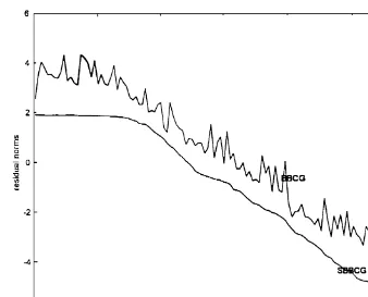
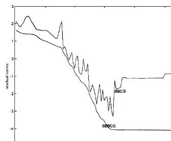
One disadvantage of the block BCG algorithm is that it often exhibits very irregular residual norm behavior. This problem can be overcome by applying the BMRS procedure to this algorithm. The smoothed block BCG (SBBCG) algorithm is given as follows:
Algorithm 2. Smoothed block BCG (SBBCG) algorithm
Y0=X0; S0=R0
Yk=Yk−1+ (Xk−Yk−1) k
Sk=Sk−1+ (Rk−Sk−1) k
where Xk is the approximation generated by the BBCG algorithm and
k=−(EkTEk)
−1ET
kSk−1 with Ek=Rk−Sk−1:
Problems of breakdowns and near breakdowns for the BBCG algorithm and the corresponding smoothed one are not treated in this work. Note also that an ecient implementation of the block iterative methods consists in delating, during the iterations, the linear systems that have been already converged.
3.3. Smoothing block FOM
In this subsection, we will show that when applying the BMRS procedure to the block full orthogonalization method (BFOM) [10], we obtain the block GMRES (BGMRES) method.
BFOM is a block generalization to the well known FOM [10]. The generated approximate Xk is
such that
and
Rik=Bi−AXki⊥Kk(A; R0) for i= 1; : : : ; s:
The sequence of residuals (Rj) produced by BFOM satises the following relation:
RT
iRj= 0; i6=j: (3.5)
BGMRES computes approximate solution X′
k of (1.1) such that kR0 −AZkF is minimized over
Z ∈Kk(A; R0). Hence the norm of the residual R′k veries
kR′
kkF= min
Z∈Kk(A; R0)kR
′
0−AZkF:
The implementations of BFOM and BGMRES are based on the block Arnoldi procedure [11]. Let us rst give a proposition that will be used in the main result of this subsection.
Proposition 5. Assume that we have an iterative block method producing a sequence of residuals such thatRT
iRj= 0fori6=j:Then the sequence of residuals (Si)generated by the BMRS procedure
satises the following relations: (i) RT
kSj=Os; j= 0; : : : ; k−1;
(ii) ST
kEj=Os; j= 1; : : : ; k; with Ej=Rj−Sj−1;
(iii) ST
kSk=SkTR0 for k¿0.
Proof. (i) The residual Sj can be expressed as Sj=
Pj
i=0Rii; j where i; j ∈Rs×s. Since RTkRi=Os
for i= 0; : : : ; k−1 it follows that RT
kSj=Os.
(ii) Is easily shown by induction.
(iii) At step k, the residual Sk can be written as
Sk=R0+
k
X
i=1
Ei i;
then multiplying on the left both sides of this last relation by ST
k and using (ii) we get SkTSk=SkTR0.
We can state now the main result of this subsection.
Proposition 6. Let(Rk)be the sequence of residuals generated byBFOM and let (Sk)be the
se-quence of residuals obtained by applying theBMRS procedure to BFOM:Then we have
kSkkF= min
Z∈Kk(A; R0)kR0−AZkF:
Proof. At step k the residual Sk can be expressed as
Sk=R0+
k
X
i=1
Ei i:
Then
=
Let B denotes the following block matrix:
Fig. 1. Matrix A1; N= 2500; s= 10.
Using the fact that RT
iR0= 0 for i6= 0 and using (i) and (ii) of Proposition 5, we obtain EiT(Si−1−
R0) = 0 for i= 1; : : : ; k and then
→
grad( ( ˜v)) = 0. This shows that
kSkkF= min
1;:::;k
R0+
k
X
i=1
Ei i
F
: (3.8)
Finally, using Proposition 4, we have Ei∈Ki(A; AR0) for i=1; : : : ; k−1. Therefore (3.8) becomes
kSkkF= min
Z∈Kk(A; R0)kR0+AZkF:
The result of this proposition shows that if the BMRS procedure is applied to BFOM, the obtained method is equivalent to the BGMRES method.
4. Numerical examples
The numerical tests reported here were run on SUN Microsystems workstations using Matlab. In these experiments, we compared the BBGC algorithm for solving problem (1.1) with the smoothed BBCG (SBCG) algorithm. The initial guess X0 was taken to be zero and the second
Fig. 2. MatrixA2; N= 1104; s= 5.
with coecients uniformly distributed in [0 1]. For the two experiments, we chose s= 10 and s= 5. The tests were stopped as soon as (kSkk=kR0k)610−7.
For the rst experiment, the matrix A1 represents the 5-point discretization of the operator
L(u) =−u+(ux+uy)
on the unit square [0;1]×[0;1] with homogeneous Dirichlet boundary conditions.
The discretization was performed using a grid size of h=1=51 which yields a matrix of dimension
N = 2500; we chose = 0:1.
In the second experiment, the matrix A2 was Scherman4 taken from the Harwell Boeing collection.
In Figs. 1 and 2, we plotted the residual norms in a logarithmic scale versus the number of iterations for the two experiments.
References
[1] C. Brezinski, M. Redivo Zaglia, A hybrid procedure for solving linear systems, Numer. Math. 67 (1994) 1–19. [2] C. Brezinski, Projection Methods for Systems of Equations, North-Holland, Amsterdam, 1997.
[3] T. Chan, W. Wang, Analysis of projection methods for solving linear systems with multiple right-hand sides, SIAM J. Sci. Comput. 18 (1997) 1698–1721.
[5] M. Heyouni, H. Sadok, On a variable smoothing procedure for conjugate gradient type methods, Linear Algebra Appl. 268 (1998) 131–149.
[6] K. Jbilou, A. Messaoudi, H. Sadok, Global FOM and GMRES algorithms for matrix equations, Appl. Numer. Math., to appear.
[7] D. O’Leary, The block conjugate gradient algorithm and related methods, Linear Algebra Appl. 29 (1980) 293–322. [8] Y. Saad, On the Lanczos method for solving symmetric linear systems with several right-hand sides, Math. Comp.
48 (1987) 651–662.
[9] Y. Saad, M.H. Schultz, GMRES: a generalized minimal residual algorithm for solving nonsymmetric linear systems, SIAM J. Sci. Statis. Comput. 7 (1986) 856–869.
[10] Y. Saad, Iterative Methods for Sparse Linear Systems, PWS Publishing, New York, 1995.
[11] M. Sadkane, Block Arnoldi and Davidson methods for unsymmetric large eigenvalue problems, Numer. Math. 64 (1993) 687–706.
[12] W. Schonauer, Scientic Computing on Vector Computers, North-Holland, Amsterdam, New York, Tokyo, 1997. [13] V. Simoncini, A stabilized QMR version of block BICG, SIAM J. Matrix Anal. Appl. 18 (2) (1997) 419–434. [14] V. Simoncini, E. Gallopoulos, An iterative method for nonsymmetric systems with multiple right-hand sides, SIAM
J. Sci. Comput. 16 (1995) 917–933.
[15] B. Vital, Etude de quelques methodes de resolution de problemes lineaires de grande taille sur multiprocesseur, Ph.D. Thesis, Universite de Rennes, Rennes, France, 1990.
[16] H. Van Der Vorst, An Iterative Solution Method for Solvingf(A) =b, using Krylov subspace information obtained for the symmetric positive denite matrix A, J. Comput. Appl. Math. 18 (1987) 249–263.
[17] R. Weiss, W. Schonauer, Accelerating generalized conjugate gradient methods by smoothing, in: R. Beauwens, P. Groen (Eds.), Iterative Methods in Linear Algebra, North-Holland, Amsterdam, 1992, pp. 283–292.
[18] R. Weiss, Convergence behavior of generalized conjugate gradient methods, Ph.D. Thesis, University of Karlsruhe, 1990.
[19] R. Weiss, Properties of generalized conjugate gradient methods, Numer. Linear Algebra Appl. 1 (1994) 45–63. [20] L. Zhou, H.F. Walker, Residual smoothing techniques for iterative methods, SIAM J. Sci. Comput. 15 (1994)