POTENTIAL OF PHOSPHORUS POLLUTION IN THE SOIL OF
THE NORTHERN GAZA STRIP, PALESTINE
Mazen Hamada1*), Adnan Aish2) and Mai Shahwan1)
1)
Department of Chemistry, Faculty of Science, Al Azhar University- Gaza P.O. Box. 1277 Gaza, Palestine
2)
Institute of Water and Environment, Faculty of Science, Al Azhar University- Gaza P.O. Box. 1277 Gaza, Palestine
*)
Corresponding author E-mail: [email protected]
Received: June 2, 2011/ Accpeted: July 27, 2011
ABSTRACT
The damage and negative consequences of the Israeli Cast Lead on Gaza in the period between December 2008 – January 2009 is not only limited to the number of martyrs and wounded people, the destruction of houses and the infrastructure, but it also reached the environ-ment. This paper investigates the occurrence of phosphorus (P) in the soil of the northern governorate of the Gaza Strip which has been shaped as a result of the heavily bombing of white phosphorus on Gaza during the war. We have measured soil Phosphorus concentrations in three different areas; agricultural, non-agricultural and urban areas. The obtained Olsen P values in most of the soil samples were ranked very high. The maximum value of phosphorous determined in agricultural areas was about 110.9 mg/ kg, in the non-agricultural areas adjacent to boarders 63.3 mg/ kg, and in urban areas 85.2 mg/ kg. The results show that the potential of phosphorus in the northern of the Gaza Strip is becoming higher than the allowed Olsen P values.
Keywords: phosphorus, soil pollution, Olsen P, Gaza Strip.
INTRODUCTION
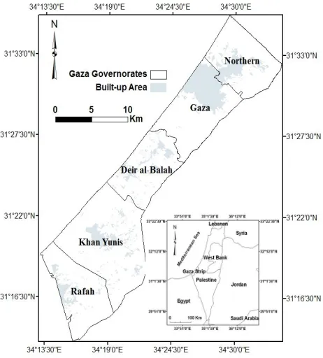
Gaza Strip is located at the south-eastern coast of the Mediterranean Sea, between longitudes 34° 2” and 34° 25” East, and latitudes 31° 16” and 31° 45” North. It is an area of about 365 km2 and it is 45 km long and its width ranges from 6 to 12 km approximately (Figure 1). It is located in the transitional zone between a temperate Mediterranean climate in the west and
north, and an arid desert climate of the Sinai Peninsula on the east and south. The population characteristics are strongly influenced by political developments, which have played a significant role in their growth and distribution along the Gaza Strip. The total population is around 1,562,000 (PCBS, 2009). Temperature gradually changes throughout the year; it reaches its maximum in August (summer) and its minimum in January (winter).
Figure 1. Location map of the Gaza Strip
The average of the monthly maximum temperature ranges between 17.6 C° in January and 29.4 C° in August. The average of the monthly minimum temperature in January is about 9.6 C° and 22.7 in August. The rainfall in the Gaza Strip gradually decreases from the north to the south. The values range from 410 mm/year in the north to 230 mm/year in the south (Aish, 2008).
Gaza topography is characterized by elongated ridges and depressions, dry stream-beds and shifting sand dunes. The ridges and depressions generally extend NE-SW direction, parallel to the coastline. Ridges are narrow and consist primarily of Pleistocene-Holocen sand-stone (locally named as Kurkar) alternated with red brown layer (locally named as Hamra). In the south, these features tend to be covered by sand dunes. Land surface elevations range from mean sea level to about 110 m above mean sea level. The geology of coastal aquifer of the Gaza Strip consists of the Pleistocene age Kurkar group and recent (Holocene age) sand dunes. The Kurkar group consists of marine and Aeolian calcareous sandstone (Kurkar), reddish silty sandstone (Hamra), silts, clays, unconsolidated sands and conglomerates (Gvirtzman et al., 1984). aquitard beneath the Gaza Strip, consisting of a sequence of marls, marine shale’s and claystones. The Kurkar group consists of complex sequence of coastal, near-shore and marine sediments. The Gaza Strip Pleistocene granular aquifer is an extension of the Mediterranean seashore coastal aquifer. It extends from Askalan (Ashqelon) in the North to Rafah in the south, and from the seashore to 10 km inland. The aquifer is composed of different layers of dune sandstone, silt clays and loams appearing as lenses, which begin at the coast and feather out to about 5 km from the sea, separating the aquifer into major upper and deep sub aquifers. The aquifer is built upon the marine marly clay Saqiye Group (Goldenberg, 1992). In the east-south part of the Gaza Strip, the coastal aquifer is relatively thin and there are no discernible sub aquifers (Melloul and Collin, 1994). The Gaza aquifer is a major
component of the water resources in the area. It is naturally recharged by precipitation and additional recharge occurs by irrigation return flow. The consumption has increased sub-stantially over the past years; the total groundwater use in year 2009 is about 165 Mm3/year, the agricultural use about 74 Mm3/year, domestic and industrial consumption about 91 Mm3/year (PWA, 2009). The ground-water level ranges between 5 m below mean sea level (msl) to about 6 m above mean sea level.
The soil in the Gaza Strip is composed mainly of three types, sands, clay and loess. The sandy soil is found along the coastline extending from south to outside the northern border of the Strip, in the form of sand dunes. The thickness of sand fluctuates from two meters to about 50 meters due to the hilly shape of the dunes. Clay soil is found in the north eastern part of the Gaza Strip. Loess soil is found around Wadis, where the approximate thickness reaches about 25 to 30 m. (Jury and Gardner, 1991).
and silt-sized material (Sharpley and Rekolainen, 1997; Quinton et al., 2001; Owens and Walling, 2002), and this material will stay in suspension longer compared to coarser material (which will also have a lower P content).
In this study, the soil-P (Olsen-P) in the northern district of the Gaza Strip after the war was determined. This was done to evaluate the change in concentration of soil-P in particular on the depth average of 0-20 cm because of its impact on water quality and associated effects on public health.
MATERIALS AND METHODS
Sampling and Sample Preparation:
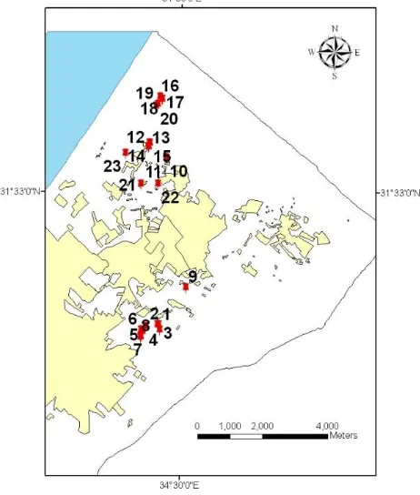
Twenty three soil samples were collected from the northern governorate of the Gaza Strip in May 2009. They were taken from different categorized areas (agricultural, non-agricultural and urban), with the help of auger to a depth of 0-20 cm. In all cases, samples were put in clean plastic bags and were homogenized. They were, then, air-dried and were passed through a mesh sieve with 2 mm openings. Figure 2 shows the locations of the soil samples taken from the northern of the Gaza Strip.
Particle Size Distribution
The particle size distribution of the soils was determined by the mechanical analysis using the Bouyoucos hydrometer, as outlined by Sheldrick and Wang (1993). Sand consists of particles >2 mm, silt of particles from 2 mm down
to 2 μm, and clay particles < 2μm. 40 g of soil
were put into a 600 mL beaker where 250 mL of ultra pure water and 100 mL of 0.5 % sodium hexametaphosphate were added. The latter reagent helped the sample be dispersed chemically. The suspension in the beaker was kept overnight. The next day, the content, helped with ultra pure water, was transferred to a dispersing cup and was mixed for 5 minutes with an electric stirrer. The sample was thus dispersed mechanically too. The suspension, helped with ultra pure water, was then transferred to a 1 L sedimentation cylinder and ultra pure water was added to take volume to 1 L. Some time was then allowed for the mixture to equilibrate thermally and a plunger was inserted to mix thoroughly. If there were foams, some drops of amyl alcohol were added. As soon as the mixing was complete
the hydrometer was lowered into the suspension and a reading was taken after 40 seconds. The mixture was again thoroughly mixed with the plunger and another reading was taken after 7 hours. The hydrometer was also lowered into a cylinder with ultra pure water only in order to take the blank reading.
Figure 2. Sample location map of the northern governorate of Gaza Strip
Calcium Carbonate (CaCO3)
The method employed for measuring the CaCO3 content of the soils was the Calcimeter
method, taken from Rowell (1994). This method is quick, simple and accurate. The Calcimeter was used to measure the CO2 evolved from the
soil samples when their CaCO3 content reacts
with 4 N HCl. The Calcimeter had previously been calibrated with standard amounts of CaCO3,
and thus the amount of CO2 which corresponds
to the CaCO3 content of the soil samples was
Soil pH
The method for measuring the pH in the soils was taken from Bascomb (1974). The pH was measured in 1 : 2.5 w/v soil : water suspension and 0.01 M CaCl2. Ten grams of soil
were weighed into a 50 mL plastic centrifuge tube and 25 mL of ultra pure water were added. The suspensions were shaken in an end-to-end shaker at 20 rpm at 21 0C for 15 minutes. The samples were, then, left to stand for 1 hour and the pH value determined using a pH meter was previously calibrated using 4.0, 7.0 and 9.2 buffer solutions.
Chemical Determination of Phosphorus in Soil
Sample Extraction
There are different extractable forms of phosphorus. According to Olsen et al. (1954), Chang and Jackson (1957), Psenner et al. (1985), Yanishevskii (1996), Sabbe and Dunham (1998), Overman and Scholtz (1999) and Reddy et al. (1999), chemically extractable forms of phosphorus include water-soluble phosphorus (WSP), readily desorbed phosphorus (RDP), algal available phosphorus (AAP) and NaHCO3
extractable phosphorus (Olsen-P). In this study Olsen-P method was used for the extraction of available phosphorous in the tested soil samples.
Determination of Moisture Correction Factor (mcf)
Before determining the p- available in the studied samples, their moisture percentage (m) and the moisture factor correction (mcf) should be determined. The results of soil analysis are to be calculated on the basis of oven dried sample weight. The determination of (mcf) was obtained as follows:
A pre-clean crucible was dried in oven at 105Co for 2 hours and then cooled down to room temperature in desiccator. At least 10g of sample were weighed and transferred into the empty
A: weight of empty crucible
B: weight of crucible + sample C: weight of dried crucible + sample
Olsen-P
A weight of 2.50 g of soil sample was placed in a glass bottle and shaken for 0.5 h with 50 mL of 0.5M NaHCO3 solution, adjusted to pH
8.5. The suspensions were filtered through 0.45mm Whatman filter membrane and the filtrates were analyzed for Olsen-P (Olsen et al., 1954; Gonsiorczyk et al., 1998). The analytical results were normalized to air-dry weight {Pf (dw)}
according to the following formula:
Pf (dw) = Pf (ww)/(1 – mcf/100) where Pf (ww) is
the wet-weight.
RESULTS AND DISCUSSION
One of the unique characteristics of phosphorus is its immobility in soil. Practically all soluble phosphors from fertilizer or manure are converted in the soil to water insoluble phosphorus within a few hours after application. However, runoff water usually contains very low quantities of soluble phosphorus, even when phosphorus is surface applied, because of phosphorus immobility in soil. In general, soil test phosphorus should be 10 – 30 mg kg-1 for the field crops and somewhat higher for potato and some vegetable crops, including cabbage, carrot, melons and tomatoes (Schulte and Kelling, 1996).
The soil types of the study area are described broadly based upon the USDA (United States Department of Agriculture) soil triangle. The types of soils found are categorized as loamy, loamy sand, sandy and sandy loam.
The pH-values of all tested soil samples ranged between 7.6 and 8.7. This shows that all of the tested soils are slightly alkaline. The widespread soil alkalinity in the tested area is due to the presence of Calcium Carbonate CaCO3 in
the soil samples. The percentage of CaCO3 found
in the samples of the agricultural areas ranges between 3.8 and 15.2, in the non-agricultural areas between 9.2 and 15.5 and in the urban areas between 2.8 and 15.8. From the above mentioned investigations, it can be concluded that the white phosphorus thrown in the tested areas is converted into P2O5 which is still
available in high concentration as soluble orthophosphates (HPO42- and H2PO4-)at the top
for slightly basic soils and this complies with our soil analysis results. The high concentration of calcium in the soil means that in the near future the surpluses of P will react with Ca to form insoluble phosphorus compounds and accumulated into deeper soil layers. In long run, these may contaminate the soil, the crops, the ground water and vegetation causing considerable adverse impact on the health of consumers and local populations.
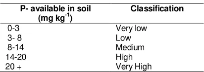
Table 1 shows the degree of classification of P available in soil according to the extracted phosphorus by Olsen-method (Bashour and El Sayeg 2007). The highest P-available should not exceed a concentration of 20 mg kg-1 soil.
The P concentration in the twenty three soil samples in different locations ranged from 2.12 mg kg-1 to 110.90 mg kg-1. In agricultural areas, the P values in all samples were ranked very high and reached a maximum of about 110 mg kg-1 as shown in Table 2. These soil surpluses of P will destroy the natural ecosystem of animals and plants and contaminate the crops products through the food chain. The farmers usually use fertilizers containing phosphorous for their crops in the tested area. The agricultural area targeted by phosphorus bombs and remnants of phosphorus bombs, which are burned by touching, were also observed during the soil sampling in this area. The concentrations of P available detected had exceeded the allowed Olson P limits.
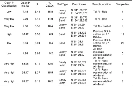
The Non-agricultural areas are located in the eastern part of invaded area where the Israeli forces had used Phosphorous bombs to cover their attacks. The potential of phosphorus in half of the samples is classified as high to very high concentrations which exceeded the allowed limits, it ranged between 16.40 mg kg-1 to 63.27 mg kg-1 as shown in Table 3. These areas should have neglected P values because they are close to the boarders where no agricultural activities are allowed.
The samples from urban areas were taken from streets and house yards in Biet Lahia which were hit by phosphorus bombs. The potential of phosphorus in samples 10, 14, 15 and 22 was very high and reached a maximum concentration of 85.8 mg kg-1.Samples number 21 and 23 were taken from areas which are not thrown by phosphorous bombs to have an interior comparison. The analysis shows that these soil samples had low concentrations as expected.
Table 4 illustrates the soil analysis results in urban area.
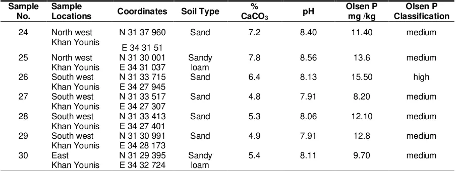
A comparison was also conducted between the study sites and areas in Khan Younis governorate in the south of the Gaza Strip, which was not hit by white phosphorus. These areas are mostly planted with citrus trees and vegetables where farmers are using fertilizers containing phosphorus. The P value measured in Khan Younis area ranged between 8.20 to 15.50 mg kg-1 as shown in Table 5. By comparing the results it was found that the P concentrations in the comparative area were much less than that of the study area and within the range level of agricultural fields
Table 1. Classification of P-available in soil according to the Olsen-method P- available in soil
(mg kg-1)
Health and Environmental Effect of Phos-phorus Weapons
Phosphorus weapons which were used in urban areas against civilians and the environment were severely damaging. White phosphorus is a highly flammable incendiary material which ignites when exposed to oxygen. White phosphorus flares in spectacular bursts with a yellow flame when fired from artillery shells and produces dense white smoke. White phosphorus has a significant, incidental, incendiary effect that can severely burn people and set structures, fields, and other civilian objects in the vicinity on fire. White phosphorus has destructive effects on the environment and also plants and may remain within the deep soil for several years without any changes.
Table 2. Analysis data for agricultural soil samples
CaCO3 Soil Type Coordinates Sample location
Sample No.
High 18.19 8.40 15.2 Loam N 31° 30,687
E 34° 29,601
Tal Al- Rais
adjacent to boarders 3
Low 3.19 8.56 18.4 Loamy
Sand
N 31° 30,74 E 34° 29,324
Tal Al- Rais /eastern
side1 of Al -Tofah 4
Bitlahia - seyafa close
the northern boarder 1 16
Very high 55.42 7.91 2.8 Loamy
Sand
N 31° 34,525 E 34° 29,627
Bitlahia - seyafa close
the northern boarder 2 17
Very high 50.53 8.11 8.2 Loamy
Sand
N 31° 34,519 E 34° 29,62
Bitlahia - seyafa close
the northern boarder 3 18
Table 3. Analysis data for non-agricultural soil samples
Olsen P Classification
Olsen P
mg /kg pH
%
CaCO3 Soil Type Coordinates Sample location Sample No.
Table 4. Analysis data for urban soil samples
CaCO3 Soil Type Coordinates Sample location
Sample
Table 5. Analysis data for agricultural area which was not attacked by Phosphorous bombs in Khan Younis
Sample No.
Sample
Locations Coordinates Soil Type
%
The potential of Phosphorous pollution after the war on Gaza was investigated in the northern district of Gaza Strip. The P values were ranked very high in most of the soil samples and exceeded the Olsen P limits. In Agricultural areas the P values in all samples were ranked very high and reached a maximum of about 110 ppm. This will destroy the natural ecosystem of animals and plants and contaminate agricultural products through the food chain. In the Non-Agricultural areas, the especially among children and the elderly.
REFERENCES
Aish, A., O. Batelaan, and F. De Smedt. 2008. Distributed recharge estimation for groundwater modelling using WetSpass model, case study Gaza strip, Palestine. Submitting to the Arabian journal for science and engineering.
Bascomb, C.L. 1974. Soil survey laboratory methods. Soil survey technical mono-graph, No 6, Harpenden, p. 14-42. Bashour, E. and A. El Sayeg. Methods for soil
analysis for arid and semi-arid areas, 2007. pp. 103.
Bell, S.G. and G.A Codd. 1996. Detection analysis and risk assessment of cyanobacterial toxins. In: Hester, R.E., and R.M. Harrison (Eds.), Agricultural chemicals and the environment. issues in environmental science and techno-logy No. 5. Royal Society of Chemistry, Cambridge. p. 109–122.
Chang, S.C. and M. L. Jackson, 1957. Fraction of soil phosphorous. Soil. Sci.84: 133-144.
Correll, D.L. 1998. The role of phosphorus in the eutrophication of receiving waters: A review. Journal of Environmental Quality 27, 261–266.
Eckert D.J. and J.W. Johnson. 1985. Phos-phorus fertilization in no-tillage corn production. Agronomy Journal 77: 789– 792.
Goldenberg, L. C. 1992. Evaluation of the water balance in the Gaza Strip. Geological survey, Report TR-GSI/16/92 (in Hebrew).
Gonsiorczyk, T., P. Casper and R. Koschel. 1998. Phosphorus-binding forms in the sediment of an oligotrophic and an eutrophic hardwater lake of the Baltic lake district (Germany), Water Science and Technology 37: 51–58.
Gvirzman,G. G.M. Martinotti, and S. Moshkovitz. 1984. Stratigraphy of the Kurkar group (Quaternary) of the coastal plain of Israel: geological survey of Israel research. pp. 64.
Jury, W. and W. Gardner. 1991. Soil physics. Fifth edition. ISBN: 0-471-83108-5. p. 4-18.
Kronvang B., A. Laubel, and R. Grant. 1997. Suspended sediment and particulate phosphorus transport and delivery pathways in an arable catchment, Gelbaek stream Denmark. Hydrological Processes 11: 627–642.
Lennox, S.D., R.H. Foy, R.V. Smith, and C. Jordan.1997. Estimating the contribution from agriculture to the phosphorus load in surface water. In: Tuney, H., O.T.Carton, P.C. Brookes, A.E.Johnston (Eds.). Phosphorus loss from Soil to water. CAB International, Wallingford, UK. p. 55–75.
Maguire, R.O., A.C. Edwards, and M.J. Wilson. 1998. Influence of cultivation on the distribution of phosphorus in three soils from NE Scotland and their aggregate size fractions. Soil Use and Manage-ment 14: 147–153.
Melloul A.J. and M. Collin. 1994. The hydro-logical malaise of the Gaza Strip. Isr. J. Earth Sci. 43(2): 105-116.
Olsen, S.R., C.V. Cole, F.S. Watanabe, and L.A. Dean. 1954. Estimation of available phosphorus in soils by extraction with sodium bicarbonate. USDA Circulation. USDA, Washington DC. pp. 939. Overman, A.R., and R.V. Scholtz. 1999.
Langmuir – Hinshelwood model of soil phosphorus kinetics. Communications in Soil Science and Plant Analysis 30: 109-119.
Owens, P.N. and D.E. Walling. 2002. The phosphorus content of fluvial sediment in rural and industrialised river basins. Water Research 36: 685–701.
Page T., P.M. Haygarth, K.J. Beven, A. Joynes, T. Butler, C. Keeler, J. Freer, P.N. Owens, and G.A. Wood. 2005. Spatial variability of soil phosphorus in relation to the topographic index and critical source areas: sampling for assessing risk to water quality. Journal of Environmental Quality 34: 2263–2277. Palestinian Central Bureau of Statistics (PCBS).
2006. Projected population in the Palestinian territory, Establishments report, Ramallah, Palestine. pp. 5. Palestinian Water Authority, 2009. Water
Psenner R., R. Pucsko and M. Sager. 1985. Die Fractionierung organischer und anorganischer Verbindungen von Sedimenten. Arch. Hydrobiol./ Suppl., 70: 111-115.
Quinton, J.N., J.A. Catt, and T.M. Hess. 2001. The selective removal of phosphorus from soil: is event size important? Journal of Environmental Quality 30: 538–545.
Reddym D.D., A.S. Rao, P.N. Takkar. 1999. Effects of repeated manure and fertilizer phosphorus additions on soil phos-phorus dynamics under a soybean – wheat rotation. Biology and Fertility of Soils 28: 150 – 155.
Rowell, D.L. 1994. Soil science: Methods and applications. Longman, Harlow.
Sabbe, W.E., and S.C. Dunham. 1998. Comparison of soil phosphorus extractants as affected by fertilizer phosphorus sources, lime recommendation and time among four Arkansas soils. Communications in Soil Science and Plant Analysis 29: 1763 – 1770.
Schulte, E.E. and K.A. Kelling. 1996. Soil and applied phosphorus, University of Wisconsin Extension PublicationA2520. Sharpley, A. 1985. Depth of surface soil-runoff
interaction as affected by rainfall, soil slope and management. Soil Science Society of America Journal 49: 1010-1015.
Sharpley, A.N. and S. Rekolainen. 1997. Phosphorus in agriculture and its environmental implications. In: Tuney, H., O.T. Carton, P.C. Brookes, and A.E. Johnston (Eds.). Phosphorus Loss from Soil to Water. CAB International, Wallingford, UK. p. 1–54.
Sheldrick, B.H. and C. Wang. 1993. Particle size distribution. In: Carter, M.R. (Ed.) Soil sampling and methods of analysis. Canadian Society of Soil Science, Lewis Publishers. p. 499-509.
Simard R.R., S. Beauchemin, and P.M. Haygarth. 2000. Potential for preferential pathways for phosphorus transport. Journal of Environmental Quality 29: 97–105.
Weil,R.R., P.W. Benedetto, L.J. Sikora, and V.A. Bandel. 1988. Influence of tillage practices on phosphorus distribution and forms in three ultisols. Agronomy Journal 80: 503–509.
Withers, P.J.A., I.A. Davidson, and R.H. Foy. 2000. Prospects for controlling diffuse phosphorus loss to water. Journal of Environmental Quality 29: 167–175. Yanishevskii, P.F. 1996. Chemical evaluation of