Dynamic Model of a Multibending Soft Robot Arm
Driven by Cables
Federico Renda, Michele Giorelli
, Student Member, IEEE
, Marcello Calisti, Matteo Cianchetti
, Member, IEEE
,
and Cecilia Laschi
, Senior Member, IEEE
Abstract—The new and promising field of soft robotics has many open areas of research such as the development of an exhaustive theoretical and methodological approach to dynamic modeling. To help contribute to this area of research, this paper develops a dy-namic model of a continuum soft robot arm driven by cables and based upon a rigorous geometrically exact approach. The model fully investigates both dynamic interaction with a dense medium and the coupled tendon condition. The model was experimentally validated with satisfactory results, using a soft robot arm working prototype inspired by the octopus arm and capable of multibend-ing. Experimental validation was performed for the octopus most characteristic movements: bending, reaching, and fetching. The present model can be used in the design phase as a dynamic simu-lation platform and to design the control strategy of a continuum robot arm moving in a dense medium.
Index Terms—Biologically inspired robots, continuum robots, dynamics, soft robots.
NOMENCLATURE
⋆ Variable in the reference configuration.
· Derivative with respect to time.
′ Derivative with respect tos. ConvertsR6 inse(3). ConvertsR3 inso(3).
t ∈RTime.
s ∈RReference arc-length parametrization.
g (s, t)∈SE(3)Configuration matrix.
ξ (s, t)∈se(3)Local deformation twist vector.
η (s, t)∈se(3)Local velocity twist vector.
ζ (s, t)∈se(3)∗Wrench twist vector.
u (s, t)∈R3 Position vector in the global reference frame.
R (s, t)∈SO(3)Orientation matrix.
q (s, t)∈R3 Local linear strain.
k (s, t)∈R3 Local spatial curvature.
v (s, t)∈R3 Local linear velocity.
w (s, t)∈R3 Local angular velocity.
N (s, t)∈R3 Internal force.
M (s, t)∈R3 Internal torque.
n (s, t)∈R3 Distributed external force.
m (s, t)∈R3 Distributed external torque.
Manuscript received December 3, 2013; revised April 14, 2014; accepted May 16, 2014. Date of publication June 9, 2014; date of current version September 30, 2014. This paper was recommended for publication by Associate Eitor and Editor B. J. Nelson upon evaluation of this reviewer’s comments. This work was supported by the European Commission within the ICT-FET OCTOPUS Integrating Project under Contract 231608.
The authors are with the BioRobotics Institute, Scuola Superiore Sant’Anna, 56025 Pisa, Italy (e-mail: [email protected]; [email protected]; [email protected]; [email protected]; [email protected]).
Color versions of one or more of the figures in this paper are available online at http://ieeexplore.ieee.org.
Digital Object Identifier 10.1109/TRO.2014.2325992
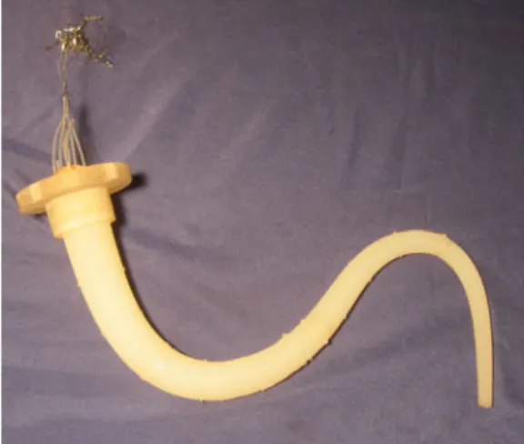
Fig. 1. Soft robot arm driven by 12 cables embedded inside the silicone body and fastened at different distance from the base. This is the prototype used for the experimental validation of the dynamic model presented in this paper.
g (s, t)∈R3Distributed gravity force.
b (s, t)∈R3Distributed buoyancy force.
d (s, t)∈R3Distributed drag force.
a (s, t)∈R3Distributed added mass force.
cl (s, t)∈R3Distributed force due to cables load.
cθ (s, t)∈R3Distributed torque due to cables load.
pi (s)∈R3Distance from the midline to theith cable in the
local reference frame.
uc (s, t)∈R3 Cable position vector in the global reference
frame.
tc (s, t)∈R3Tangent vector to the cable.
uj (t)∈R3 Position vector of thejth reconstructed marker.
I. INTRODUCTION
C
ONTINUUM soft robots are a class of robots almost com-pletely made of soft elastic materials (see Fig. 1). They may be regarded as the natural evolution of hyperredundant snake-like robots [1] with a completely soft structure of infinite degrees of freedom (DOFs), intrinsically underactuated and ex-tremely adaptable to the environment [2]. A continuum robot arm changes shape during operation and shows continuum bend-ing, allowing both positioning in space and interaction with the environment (e.g., object manipulation [3], walking [4]).This kind of robot arm is undoubtedly promising, especially in the field of autonomous intelligent robots, where robots need to operate in an unstructured environment. Indeed, they are 1552-3098 © 2014 IEEE. Personal use is permitted, but republication/redistribution requires IEEE permission.
intrinsically safe; they comply with the environment and do not need a fine and heavy control architecture.
Furthermore, their infinite DOFs can be exploited to obtain dexterous behavior in constrained environments, enabling them to be applied to new industrial fields.
Numerous examples of continuum robots can be found in [2]; among these, some of the most popular examples are the octopus-inspired robot arm described in [3] and the elephant trunk robot arm in [5].
Since soft robot shapes are affected significantly by external loads [2], a dynamic model is fundamental for exploiting the effect of these loads in the execution of a task. In order to model continuum robot arms, traditional mathematical tools, typically used for robot dynamic modeling, cannot be applied. A contin-uum approach is required, with distributed parameters instead of concentrated parameters, and nonlinear partial differential equations need to be considered. In the robotics field, existing models can be divided into two main categories: constant and nonconstant curvature approximation. They vary in the degree of precision obtained. The constant curvature approximation can be considered as the simplest approach to modeling soft robots. As specified in various constant curvature works (see [6]–[8]), this approximation fails in many practical cases, for example, when the environmental loads (such as gravity) are significant or in the case of nonconstant sections of the robot arm. For cable-driven robot arms, the constant curvature approximation also fails in the coupled tendon condition [9]. For a detailed review of piecewise constant-curvature approximation works, see [6]. Among them, the most significant achievements for this study are reported in [7] and [9], where an exhaustive analysis of tendon actuation is given and the control system is shown, for a cable-driven continuum manipulator. Another application of the constant curvature approximation is described in [8] for a pneumatic continuum manipulator.
Nonconstant curvature models belong to three categories: continuum approximation of hyperredundant systems [10]– [12], the spring–mass model [13], [14], and the Cosserat ge-ometrically exact approach [15]–[23].
Continuum approximation of hyperredundant systems was probably the first continuum approach to be proposed in the robotics community, unveiling a variety of applications such as snake locomotion [10] or trunk manipulation [11], [12]. How-ever, the latest robotic platforms developed, which are made of highly deformable continuum bodies, have led quite natu-rally to using a pure continuum approach to modeling from the beginning.
Regarding spring–mass models, they cannot reproduce the majority of actuation principles; they present heavy computa-tional efficiency problems and need to be experimentally cali-brated for every new application. However, this kind of model has been successfully applied to describing biological contin-uum arms as in [14].
Cosserat geometrically exact models are the closest to the mechanics of continuum robot arm structures and actuation. For this reason, this approach was chosen for the study.
The state of the art on Cosserat geometrically exact mod-els for soft robot arms has been limited so far to static
analysis [17], [19], [22], [23] or to the theoretical presen-tation of dynamic cases, without performing simulations or experimental comparisons [16], [18], [20] and without consider-ing external dynamic loads such as drag forces and added mass forces. On the contrary, regarding locomotion, in [15], the ge-ometrically exact model of a Cosserat beam, whose strains are imposed by control torques or constraint forces, is proposed. The resulting dynamics is that of a continuous rigid multi-body system which can be solved with a continuous version of the (Newton–Euler-based) Luh algorithm [24]. Once coupled to the elongated body theory of Lighthill [25], this approach solves the dynamics of a self-propelled swimming hyperedun-dant fish-like robot [15]. More recently, in [21], the controlled strains of [15] were replaced by passive strains governed by constitutive laws, and the Lighthill model was extended to the case of a nonquiescent fluid. Again, the use of a Newton–Euler-based algorithm allowed the authors to address the case of a dead fish passively swimming in a von Karman Vortex Street. In all these cases, some of the strains of the general Cosserat beam model are forced to zero, and the resulting model is that of an inextensible Kirchhoff beam (i.e., with no transverse shear-ing). On the contrary, in this paper, all the strains of the Cosserat model are governed by strain-stress laws, including stretching which drastically changes the shape of equations. Remarkably, in this case, since there are no longer any internal constraints, the Newton–Euler algorithms can be circumvented by using a simple finite-difference resolution. Furthermore, while in all these works the problem of the technological implementation of actuation is not addressed, in this paper, a recently developed efficient solution based on cables is proposed [26]. Finally, the paper goes beyond these theoretical works by assessing the proposed model through comparisons between simulations and experiments.
In addition, although theoretically considered, previous works show simulations of Cosserat beam with constant generalized elasticity [16] (constant elasticity and constant section), while nonconstant elasticity, as simulated in this study, leads to con-tinuum robot arms that are more suitable for grasping objects, as described in [27].
In further detail, this study provides a complete description of the loads that can be applied to a continuum robot. The model addresses all the hydrodynamic forces exerted on a robot arm moving in a dense medium, i.e., buoyancy, drag, and added mass forces. Moreover, the strains of the Cosserat model are gov-erned by a specific linear viscoelastic constitutive law (Kelvin– Voight), while related mechanical tests on the material are pre-sented. Finally, to the best of our knowledge, this is the first time in the continuum robotics literature that a dynamic experimental validation is performed, with a working prototype driven by 12 cables (see Fig. 1), inspired by the octopus arm [26], modeled by a geometrically exact beam and with nonconstant generalized elasticity.
by the discussion of the results. Finally, the last section is left for the conclusions. A complete summary of variables and operators is given in the Nomenclature.
II. THEORETICALFRAMEWORK
In the geometrical exact approach, a robot arm is viewed as a Cosserat rod. Outside robotics, there is a vast literature on the dynamical theories of Cosserat rods, in particular [29]–[32] should be considered for a detailed derivation of the Cosserat beam theory. The relevant features for soft robotics applications have been extrapolated from this vast literature and are presented in the following sections. Below, the kinematics and dynamics of the Cosserat rod theory are described using geometrical formu-lation and notations [28], [33]. For a useful and recent reference to the geometric literature in continuum robotics, see [34].
A. Kinematics
In the Cosserat rod theory, the configuration of a beam at a cer-tain time is characterized by a position vectoru(s, t)∈R3and a material orientation matrixR(s, t)∈SO(3), parameterized by the material abscissas∈[0, L]⊂Rand timet∈[0,∞)⊂R, whereLis the total length of the robot arm. Thus, the robot arm configuration space is defined as a functional space of curves
g(s, t)∈SE(3), with
The tangent vector field along the curve g(s, t) is defined by ξ(s, t) =g−1∂g/∂s=g−1g′. It is an element of the Lie
algebrase(3)of the Lie groupSE(3). The hat represents the isomorphism between the twist vector spaceR6 andse(3):
k(s, t)∈R3represents the angular strain measuring the bend-ing and the torsion state of the beam. The tilde is the usual isomorphism between a vector of R3 and the corresponding skew-symmetric matrix.
In the case of straight reference configuration, the undeformed space twist is constant and equal to ξ⋆ = (0,0,0,1,0,0)T
(where ⋆ denotes any quantity evaluated in its reference con-figuration). Sinceξ⋆ is the tangent field ofg⋆, this means that
the rotational component ofg⋆(s)(i.e., inSO(3)) is constant
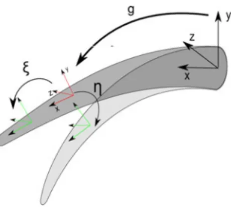
and that the local first axisxhas been fixed perpendicular to sections (see Fig. 2). On the other hand, the other two local axes can be placed arbitrarily on the plane of the section. Below, we will assume that they lie along the principal inertia axis of the cross section with the origin of the local reference frame placed at the centre of the circular sections.
Fig. 2. Sketch visualization of the kinematics and the geometrical meaning of the elementsg,ξ, andη. The reference frames on the figure are those used in the model.
Looking at the fixed reference frame of Fig. 2, the following reference configuration was considered:
The time evolution of the configuration curve g is rep-resented by the twist vector field η(s, t)∈R6 defined by velocity, respectively, of a material element at a given instant.
In accordance with these kinematics, the time evolution of the rod-like robot arm is determined by the twist vector fieldη, shown as follows:
˙
u=Rv, R˙ =Rw. (1)
For a sketch representation of the kinematics, see Fig. 2.
B. Compatibility Laws
We have seen above thatg′=gξ. By taking the derivative of this equation with respect to time and recalling thatg˙ =gη, we obtain the following compatibility equation between velocity and deformation variables:ξ˙=η′ +ξη−ηξ. In terms of twist
Finally, by splitting it into linear and angular components, and rearranging the terms, we obtain
˙
q =v′+k×v−w×q
˙
k =w′+k×w (2)
which are the compatibility laws used in the model.
C. Dynamics represent the density of the rod and the section area, respectively,
Iis the identity matrix, andJ(s)∈R3⊗R3 is the second mo-ment of the area tensor, which is equal toJ = diag(Jx,Jy,Jz).
Jy(s),Jz(s)∈Rare the second moments of the area of the rod
cross section with respect to axisyandz(equal toπr4/4for
a circular cross section with radiusr(s)∈R), andJx(s)∈R is the polar moment of the area around the axis x equal to
Jx =Jy +Jz.
Let us callζi(s, t)∈se(3)∗the wrench of forces applied by
the left part (x < s) into the right part (x≥s) of the beam, across sections. By taking the derivative ofζiwith respect to
s, we obtainζ′
The equilibrium on the infinitesimal material elementdsis given by the internal wrench of forces and the external wrench of distributed applied forcesζ′
i−ad∗ξ(ζi) +ζe′. By the laws of
Newtonian mechanics, we know that the total wrench of applied forces is equal to the fine-rate of change of the kinetic wrench; thus, by taking the derivative w.r.t.tof the kinetic wrench, we obtain the following dynamics equation:
ζ′
i−ad∗ξ(ζi) +ζe′ = Γ ˙η−ad∗η(γ). (3)
Let us specify the angular and linear components of the in-ternal and exin-ternal wrenches: the external force and torque for unit ofs.
By splitting (3) in the linear and angular components and rearranging the terms, we obtain
N′+k×N+n=ρAv˙ +w×ρAv
M′+k×M+q×N+m=ρJw˙ +w×ρJw.(4)
Once multiplied bydson both sides, (4) corresponds to the classical Newton equations applied to the infinitesimal piece of beamds.
D. Constitutive Laws
The internal force and torque can be related through material constitutive laws to the mechanical strains. These strains are defined as the difference between the deformed configuration (ξ) and the reference configuration (ξ⋆).
In particular, the components ofk−k⋆ measure the torsion and the bending state in the two directions. Similarly, the com-ponents ofq−q⋆ represent the longitudinal strain (extension, compression) and the two shear strains.
Linear constitutive equations for an isotropic hyperelastic ma-terial were chosen both for the elastic and the viscous members, and no bulge effects were considered. This simple approach is justified by the intended aim of this model for robotics appli-cation, that is, to describe the global dynamics and geometric properties of the system, neglecting details on material behavior. The simplest viscoelastic constitutive model is the Kelvin– Voigt model, which simply adds a viscous contribution linearly, proportional to the rate of strain, to the elastic contribution:
ζi= Σ(ξ−ξ⋆) + Υ( ˙ξ), whereΣ(s)andΥ(s)∈R6⊗R6are,
respectively, the screw stiffness matrix and the screw viscosity matrix equal to G∈Rare the Young modulus and the shear modulus, respec-tively. For an isotropic material, we have G=E/2(1 +ν), whereν∈Ris the Poisson ratio.
According to [35], elastic and viscous contributions have the same form. In the case of 1) moderate curvature of the rod in its reference configuration, 2) strain rates that vary slowly com-pared with the internal relaxation processes, and 3) a homoge-neous isotropic material, an explicit formula for the damping parameters of the model can be obtained in terms of stiffness parameters and retardation time constants, which are defined as the ratios of the shear viscosities w.r.t. the elastic moduli. Thus, for an incompressible material (ν= 0.5), the following expres-sion holds:R3⊗R3 ∋Vl(s) = diag(3μA(s), μA(s), μA(s)),
R3⊗R3∋Vθ(s) = diag(μJx(s),3μJy(s),3μJz(s)), where μ∈R is the shear viscosity that can be formulated in terms of the retardation time constant (τ) asμ=Eτ /3.
Expressed withR3vectors, the constitutive equations are the following:
N=Kl(q−q⋆) +Vlq˙,culoM=Kθ(k−k⋆) +Vθk˙.
(5)
III. EXTERNALLOADS
This section will analyze the external loads taken into account for the present model.
Finally, the external load represented by the action of the cables on the robot arm will be analyzed.
Equation (6), as seen below, shows how these loads form the termsnandmof the equilibrium equations (4)
n=g+b+d+a+cl,culom=cθ (6)
whereg(s, t)∈R3is the gravity load,b(s, t)∈R3is the buoy-ancy, d(s, t)∈R3 is the drag load, and a(s, t)∈R3 is the added mass load. Finally, the action of the cables can be divided into distributed force and torque component namedcl(s, t)and
cθ(s, t)∈R3, respectively.
The hydrodynamic model is essentially that developed in [15]. This model accounts for added mass, buoyancy (and grav-ity) along with drag forces. While the first two models (added mass and buoyancy forces) are entirely deducible from alge-bra based on the assumption of the ideal fluid (incompressible, unviscous) and on the high aspect ratio (length/radius) of the arm, the theoretical modeling of drag forces has not yet found a closed solution (based on the boundary layer theory). As a result, the drag forces are modeled with an empirical model due to Morisonet al.[36]. The complete model was validated through extensive Navier–Stokes simulation in the case of the self-propelled swimming of an elongated fish in [37].
A. Gravity and Buoyancy
Gravity and buoyancy are simply the product between the mass per unit ofs, respectively, of the robot armρand of the mediumρw ∈R, and the gravity accelerationgr∈R. As shown
in (7), the resultant vector is rotated to the local reference frame, according to
g+b= (ρ−ρw)ARTG (7)
where Gis the gravity acceleration vector expressed asG= (0,−gr,0)T in the fixed frame.
B. Drag Load
The drag load vector is proportional to the square of the velocity vector and is directed in the opposite direction. The amplitude of the drag load is also determined by the geometry of section sand by hydrodynamics phenomena expressed by empirical coefficients. Equation (8) shows the resultant vector used in this model:
d=−ρwvTvD
v
|v| (8)
whereD(s)∈R3⊗R3 is a tensor which incorporates the ge-ometric and hydrodynamics factors in the viscosity model. It is equal toD= diag(1
2πrCx,rCy,rCz)for circular cross
sec-tions, wherer(s)∈Ris the radius of the sections, andCx,Cy,
Cz ∈Rare the empirical hydrodynamic coefficients.
In the case of circular cross sections, the drag forces produce no moment on the cross section.
C. Added Mass Load
The added mass load vector is proportional to the acceleration vector and is directed in the opposite direction. As in the case of
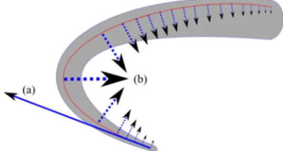
Fig. 3. Sketch of the cable loads. (a) Concentrated load where the cable is fastened. (b) Distributed load along the path of the cable inside the robot body.
the drag load, the amplitude is also determined by the geometry of section s and by hydrodynamics phenomena expressed in part by correction coefficients.
For a circular cross section, the added mass load does not have an angular component. Furthermore, the x linear component is neglected because transversal acceleration is low (there is no global movement, just deformation). Equation (9), as seen below, shows the resultant added mass vector used in this model:
a=−d(ρwFv)
dt =−ρwFv˙ +w×ρwFv (9)
where F(s)∈R3⊗R3 is a tensor which incorporates the geometric and hydrodynamics factors. It is equal to F =
diag(0, ABy, ABz), whereBy and Bz ∈R are the
hydrody-namic correction coefficients for the added mass model.
D. Cable Load
A cable acts on the robot arm in two different ways: by a con-centrated load where the cable is fastened (ins¯) [see Fig. 3(a)] and by a distributed load along the cable path inside the robot arm body [see Fig. 3(b)]. The former has an amplitude equal to the cable tension T(t)∈R and is directed in the opposite direction with respect to the cable tangent vector −Ttc(¯s) .
The latter is proportional to the cable tension and to the cable bendingTtc′(s)[7].
To model these loads, we need to define the kinematics of the cables. Since the cables are embedded inside the robot body, their relative position with the robot arm midline re-mains constant. Thus, we can define the cable position vector
uc=u+Rp, wherep(s)∈R3 is the local distance from the
midline to the cable at a certain section s(px= 0 holds; see
Fig. 4).
Unlike rods, cables do not present shear strains due to the low thickness of the cross section. This allows us to derive the vector tangent to the cabletc(s, t)∈R3simply by taking the derivative
of the position vector with respect tosand normalizingtc=
uc′/|uc′|.
With this expression at hand, the concentrated and distributed load exerted by the cable (ζecc(s, t),ζec′(s, t)) can be calculated:
ζecc =Ad∗g(ζeccr ) =
−p×T RTt c
−T RTt c
ζec′=Ad∗g(ζecr ′) =
p×T RTt c′
T RTt c′
Fig. 4. Design parameters of the prototype, cable numbering, and their posi-tions inside the silicone body.
where
are the concentrated and distributed cable load in the fixed frame as defined previously, and
Let us highlight the force and torque played by a cable an-chored ins¯:
IV. MULTIPLEBENDINGDYNAMICMODEL
At this point, all the elements of the model have been il-lustrated. Here, the system of second-order partial differential equation is reported in the state form∂z/∂t=f(z, z′, z′′, t): The kinematics equations (1), the compatibility equations (2), and the dynamic equations (4) can be recognized. The dynamic
equations are deduced from the space derivative of the constitu-tive equations (5) and the external loads (6), in turn composed by (7)–(9) and (10). The above partial differential equations would be of first order if elastic (and not viscoelastic) constitutive equations were considered.
A. Multiple Cable and Discontinuity
The present model is suitable for managing the multiple cable and coupled tendon issue. In the case ofkanchorage sections andhcables per section, the external loadsnandmchange as follows:
In addition, for every anchorage cross section, the contribution of the concentrated loads of the cables fastened there has to be added. Mathematically, for thekth anchorage section, placed in
s=Lk, we have The apices+,−indicate, respectively, the positive and negative limit of the dynamic (4).
B. Boundary Conditions
Att= 0, the robot arm is in relaxed configuration; thus, all the quantities are known: u(s), R(s), q(s), k(s), v(s), and
w(s). In the simulations below, the relaxed configuration is the equilibrium position, which is reached when the prototype is subject to gravity.
Ats= 0, the robot arm is fixed to a mobile base and the so-called kinematics boundary condition is obtained, and∀tv(0) andw(0)are known. In the simulations below, a static base was chosen.
Finally, ats=L, the so-called static boundary condition is obtained, and∀tq(L)−q⋆(L)andk(L)−k⋆(L)are known. Since there are no tip loads in our model (if the small tangential drag load is neglected), the following holds:q(L)−q⋆(L) = (0,0,0)T, andk(L)−k⋆(L) = (0,0,0)T.
C. Numerical Scheme Analysis
The simulation process starts with the choice of the cable tensions in timeT(t). At every time step, the space derivatives ofv,w,q,k,q˙, andk˙ are numerically calculated by a forward (from base to tip) finite differentiation forv andw and by a backward finite differentiation for the others. Afterward, the model equations (12) are integrated.
and a decentralized space differentiation (Upwind). Here, we used a second-order Runghe–Kutta time integration (by means of theode23function), a right (toward the tip) differentiation forvandw,and a left (toward the base) differentiation forq,
k,q˙, andk˙; under this condition, we obtained a truncation error ofO(dt2+ds).
With the artificial diffusion idea in mind [38], the choice be-tween forward and backward differentiation was made follow-ing the information flow direction of these variables led by the boundary conditions. The so-called kinematic (v,w) boundary condition was obtained at the base and the static (q,k) boundary condition at the tip (see Section IV-B).
The necessary condition for the stability of the explicit nu-merical scheme is represented by the Courant–Friedrichs–Lewy condition, which states that dtds/|v1| for the first-order
member anddtds2/|v
2|for the second-order member, where |v1|and|v2|are the largest velocity coefficients of the hyperbolic
equations that in our case are|v1|=
E/ρand|v2|= 3μ/ρ.
The model was run on an AMD Phenom(TM) II X4 965 processor, at 784 MHz and 3.25 GB of RAM, and took on average of 28 min for 1 s of simulation. This time could probably be improved by parallelizing of the integration process, i.e., by dedicating and synchronizing different cores for the time integration of every material point of the discretization.
V. EXPERIMENTALVALIDATION
The following paragraphs describe the working prototype (see Fig. 1) and the experimental setup, as well as the 3-D video reconstruction process used to extract the experimental data.
A. Multiple Cables Prototype
The prototype is composed of a single conical piece of sil-icone (that represents our Cosserat rod) actuated by 12 cables immersed inside the robot body. Let us call the base radius
Rmax and the tip radiusRm in ∈R. Since the entire robot body
is made of silicone, E,G,ν,μ, and ρare constant along s. Nevertheless, the viscoelasticity of the rod is not constant due to the reduction of the circular section area alongs.
The geometric proportion between the robot arm and the real octopus arm is similar. The silicone densityρis close to biological tissue density, and the cables play the role of the longitudinal muscle of the octopus arm.
The cables are anchored four at a time at three different lengths along the robot arm. Let us call themL1,L2, andL3 ∈R
from the base to the tip (see Fig. 4). For each anchored section, a circular piece of rigid polymer is immersed in the arm section, which allows the cross fixing of the four cables and presents appropriate holes allowing the rest of the cables to reach their own anchoring points.
For further details on design and fabrication, a similar proto-type has been presented in [26].
Let us callpi(s)∈R3 the distance from the midline to the
cablei∈[1,12]⊂N(see Fig. 4). We havepi(s) =piconstant
∀i, and|pi|=|pj|for the four cables of the same anchorage
section, i.e., the amplitudes are the same. Furthermore, we have
pi/|pi|=pj/|pj|for the three cables of different anchoring
TABLE I
DESIGNPARAMETERS OF THEPROTOTYPESILICONEBODY
Parameter Value
Rm a x 15 m m
Rm i n 4 m m
L 418 m m
L1 98 m m
L2 203 m m
L3 311 m m
k 3
h 4
E 110 kPa
μ 300 Pa·s
ν 0.5
ρ 1.08 kg/dm3
TABLE II
DESIGNPARAMETERS OF THEPROTOTYPECABLES
Cable pym m pz m m
1 −9 0
2 0 −9
3 9 0
4 0 9
5 −6 0
6 0 −6
7 6 0
8 0 6
9 −3 0
10 0 −3
11 3 0
12 0 3
TABLE III
ENVIRONMENTPARAMETERS(Re≃104)
Parameter Value
ρw 1.022 kg/dm3
g r 9.81 m/s2
Cx 0.01
Cy 2.5
Cz 2.5
By 1.5
Bz 1.5
section but on the same side, i.e., the directions are the same (see Fig. 4).
For the values of the design parameters described previously, see Tables I and II.
The prototype works in water, characterized by the parameters summarized in Table III.
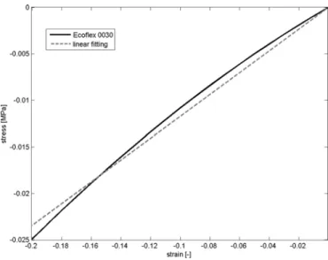
Fig. 5. Stress-strain plot of experimental compression tests on 0030 Ecoflex and linear fitting (slope=0.117, RMS error=0.9904).
Fig. 6. Experimental setup. (a) Servomotors, (b) force sensors, (c) cables, (d) L-shape supporting structure, (e) LED, (f) silicone robot arm, (g) moving marker, and (h) fixed marker.
data available for commercial elastomers typically ranging from tens to thousands of Pa·s.
The specific viscosity measures of the silicone used here (Smooth-On Ecoflex 0030) were planned, since the technical data sheet of the product gives no numerical reference of vis-cosity after polymerization. Nevertheless, a dynamic method (such as the oscillatory strain) should be used, because the typ-ical relaxation time of a silicone (τ = 3μ/E) is in the order of tenths of a second, which limits the use of a static method as creep [40].
B. Measurement Setup
The arm [see Fig. 6(f)] is lodged on a supporting structure and is immersed in a tank filled with water. The robot arm is actuated
by the 12 cables [see Fig. 6(c)] attached to four servomotors [see Fig. 6(a)] at a time, depending on the movement performed. The cable tensions are measured by four force sensors [see Fig. 6(b)], positioned on the supporting structure. The servomotors are driven by a microcontroller, which implements a control routine based on a PID regulator. The reference signals for the PID controller are the desired cable tensions, which are sent from a laptop connected to the microcontroller by a serial protocol. When the test starts, an LED [see Fig. 6(e)] attached outside the tank lights up.
1) Supporting Structure: The supporting structure [see Fig. 6(d)] is composed of two parts: a Perspex plate, where the servomotors are fixed, and a L-shape structure of aluminium, which holds an adjustable base, where the prototype is fixed.
The cables are pulled by servomotors. A pulley system is used to decrease the friction between the cables and the supporting structure. The force sensors are connected by the cables to the servomotors on one side and to the robot arm on the other side. Since the force sensors are fixed near the servomotors, they can measure the tension of the cables at that specific position. They cannot provide in-formation about force dissipated through friction along the structure.
2) Hardware and Software Systems: The core of the hard-ware system is the Ingenia Communication Module iCM4011, based on dsPIC30F4011, which is a 16-bit RISC micro-controller with an oscillator frequency of 7.37 MHz. The microcontroller takes as input the voltages provided by the am-plifier of the four force sensors and commands four servomo-tors (HS-785HB Hitech) via its digital ports. The servomoservomo-tors and the sensors are supplied by a 5-V voltage reference. The force sensor used for this application is an S-beam load cell built by Futek (model FSH00103). The sensor has a capac-ity of 22 N and a sensitivcapac-ity of 2 mV/V, and it shows negli-gible nonlinearity and hysteresis effects. The amplifier mod-ule (2039 Ministrain built by Meco) is composed of a voltage regulator for the sensor power supply and an amplifier stage with a fixed gain of 500, a trimmer for zero regulation, and a low-pass filter (0–1 kHz). A program developed in C language was purposely created to implement the digital controller (PID) on the dsPIC. The reference signals for the PID regulator are the desired cable tensions, which are sent from a laptop via the serial protocol RS-232. A program is executed on the lap-top to perform the robot movement. The program, written in M-code sends the desired cable tensions with an appropriate timing and receives the sensor values, which are stored in a text file.
C. Three-Dimensional Video Reconstruction
reference frames as the object-space reference frame, inxyz
coordinates, and the image-plane reference frame, inuv coor-dinates. Rearranging from [41], the equations that map the two reference frames are
u= H1x+H2y+H3z+L4
H9x+H10y+H11z+ 1
v= H5x+H6y+H7z+H8
H9x+H10y+H11z+ 1
(14)
whereH1. . . H11 are calledDLT parameters, and they reflect
the relationships among the 3-D coordinates of the object-space reference frame and the 2-D coordinates of the image-plane reference frame for a specific two-camera system. Note that
H1. . . H11 represent the physical parameters of the cameras
settings: They need to be derived through a calibration process to allow reconstruction.
The camera settings applied here are the same as those used in [4]. Two cameras, 11 DLT parameters, and eight fixed markers [see Fig. 6(h)], calledcontrol points, which define the calibration frame, were used. The calibration frame has a volume of about 125dm3, and all the arm movements belong to this volume. It is worth mentioning that, since calibration is an iterative process, in order to obtain the 11 DLT parameters using the least-squares method, the minimum number of control points required is 6. However, by increasing the redundancy of the system, the accu-racy of the reconstruction increases; thus, eight control points were used.
Once the DLT parameters are identified, reconstruction is possible. Four markers [see Fig. 6(g)] were placed along several sections of the arm, plus one reference marker was placed on the base of the arm. This latter marker did not move during the experiments. Two high-speed cameras (100-fps temporal resolution, 1240 × 1000 spatial resolution, black and white acquisition) were used. Anad hocsoftware was developed to automatically extract the 2-D position from the images and then perform 3-D reconstruction. The cameras were positioned to avoid occlusions as much as possible; however, when occlusion occurred, the markers were extracted manually.
VI. RESULTS ANDDISCUSSION A. Trials and Measurements
The same inputs (tension of the cables) were applied to the real prototype and to the model. Then, the trajectories of four markers placed on the robot arm atL1, L2,L3, and Lwere
compared between the two. This process was repeated for sev-eral cases of study inspired by the octopus’ most characteristic movements: bending, reaching [14], and fetching [39]. Bending is the creation of a global curvature along the full arm length. Reaching is the propagation of a strong local bend from the base to the tip. Fetching is the movement with which the octo-pus brings food to the mouth, located at the base of the arms, obtained by two opposite bends that create three segments.
Two types of errors were defined: the mean errorem(t)∈R,
as the mean normalized summation at each time step of the Euclidean distance between the relatives simulated and real markers, and the tip error et(t)∈R, as the normalized
Euclidean distance between the model and prototype tip po-sition
et(t) = |
u(L, t)−u4(t)| L
em(t) =
et(t) +3j= 1|u(Lj, t)−uj(t)|/L
4 . (15)
The former is an effective indicator of the mean distance between the real and simulated configuration of the prototype, while the latter provides the robotics community with a more appropriate accuracy evaluation, since it indicates the traditional end effector position error. Moreover, the tip distance is almost always the largest one because a bending error occurring on the robot arm length is integrated and amplified toward the tip.
In (15),uj(t)∈R3 is the reconstructed position of thejth
marker, andu(Lj, t), in this case, represents the position of the
jth simulated marker, which is not exactly the position of the midline ats=Lj, since it is located on the surface of the robot
arm.
Starting from reference measurements and parameters, the model was calibrated manually by shaping the material param-eters ρ,μ,E (see Table I) and the hydrodynamic coefficients
Cy,Cz,By, andBz(see Table III).
The model was tested by performing the three different move-ments: bending, reaching, and fetching; the former two are pla-nar movements, while the latter is a 3-D movement (which could also be performed as a planar movement; we decided to choose a 3-D movement to properly test the feasibility of the model).
In order to reproduce these behaviors in our prototype, a different number of cables were pulled at the same time (one cable for bending, two cables for reaching, and three cables for fetching) at different anchoring levels. This allowed the multibending properties of the model to be simulated and tested.
B. Results
The model was compared with experimental data with satis-factory results.
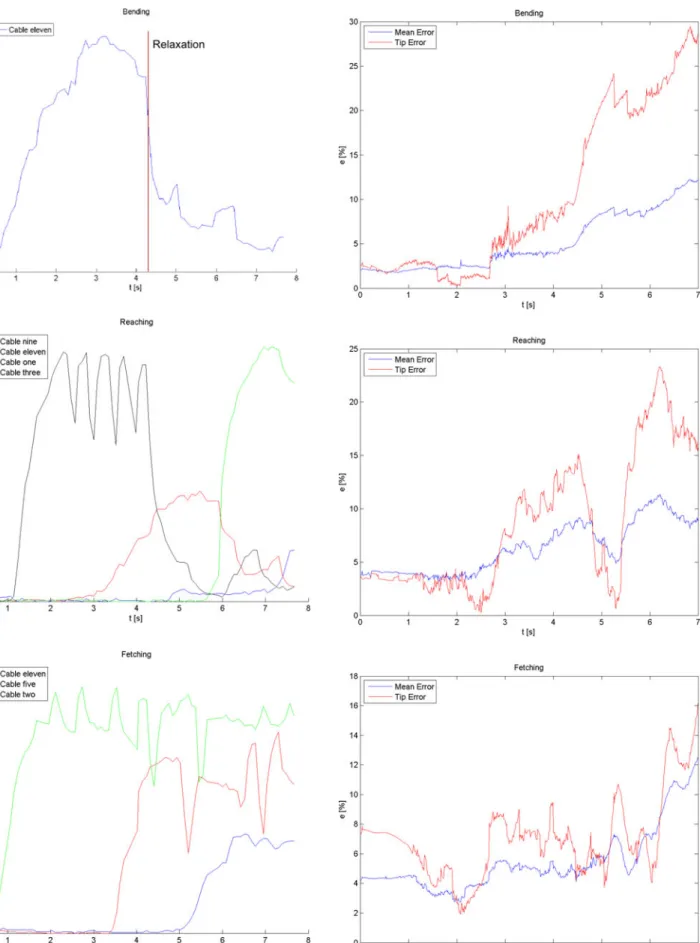
1) Bending: Cable 11 (see Fig. 4) was pulled to a tension of
∼2 Nfor 4 s and then released for the rest of the test [see the top of Fig. 7]. The trend of the mean and tip error defined in (15) is reported at the top of Fig. 8.
2) Reaching: Cables 3, 11, 1, and 9 (see Fig. 4) were pulled sequentially to a tension of, respectively,∼4 N,∼2 N,∼4 N, and∼1 N. The cables were activated with an interval of 2 s between one another, and, once they reached the desired strength, the tension was held for 3 s, for cables 3 and 11, and 1 s, for cables 1 and 9 [see the middle of Fig. 7]. Only two cables were pulled at the same time. The trend of the mean and tip error is reported in the middle of Fig. 8.
Fig. 7. Graphics of the cables tension versus time. From the top: cable 11 of the bending test; cables one, three, nine, and 11 of the reaching test; and cables two, five, and 11 of the fetching test.
TABLE IV
EXPERIMENTALVALIDATIONRESULTS
Test Mean Error Tip Error Bending 5.1% 10.3%
Reaching 5.2% 8.5%
Fetching 5.4% 7.0%
Bending
(actuated phase) 2.7% 3.4%
In all the tests, both the real and the simulated robot arm start from the equilibrium position that is reached when the prototype is subject to gravity only.
C. Discussion
When analyzing the results of Fig. 8 (whose values are re-ported in Table IV), an average (in time) mean error of5.1%, 5.2%, and5.4%was found for the bending, reaching, and fetch-ing tests, respectively. These indexes approximately express the mean distance between two curves in space: real and simulated. The tip error was calculated to provide a more common ac-curacy index for the robotics community. As shown in Fig. 8, an average tip error of10.3%,8.5%, and7.0%was found for the bending, reaching, and fetching tests, respectively. These errors are acceptable for a continuum soft robot arm in dynamic conditions, as they sum up the small bending errors along the arm length due to the level of complexity of the model. The videos attached show the similarity between the behavior of the prototype and of the model. These tests represent a starting point for future analysis, since for the first time in the continuum robotics literature, physical experiments have been performed to evaluate the transient response of a dynamic rod model of a robot.
The errors measured during the validation trials may derive from several parts of the system. The authors believe that the limited approximation and simplification adopted in the model represent a minor source of errors, whereas the fabrication of the prototype with soft materials introduces some relevant drawbacks and poorly controllable inaccuracies, as analyzed by Giorelliet al.[27]. Another source of errors may derive from the lack of systematic parameter identification, because of the high computational time of the model.
The authors, however, believe that the most important source of errors is the lack of a friction model in the simulations. Friction occurs upon contact between the cables and the silicone body and between the cables and the rigid polymer part of the anchoring section. In the second part of the bending test, the relaxation of the robot arm is driven by friction only, since the tension is close to zero [see the top of Fig. 7]. In this part, the difference between the model and the real data increases significantly. When the average errors of the bending test were calculated for the actuated part only, the mean and tip error were 2.7%and3.4%, respectively, i.e., less than half of the result of the complete test (see Table IV).
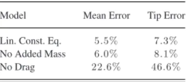
TABLE V WORSENEDMODELRESULTS
Model Mean Error Tip Error Lin. Const. Eq. 5.5% 7.3%
No Added Mass 6.0% 8.1%
No Drag 22.6% 46.6%
D. Worsened Model Analysis
In order to investigate which parts of the model are more significant, different chopped models were compared with re-spect to the fetching experimental data, which are the most exhaustive among the others. The model was evaluated with a linear elastic constitutive law [μ= 0in (5)], in the absence of added mass load [By =Bz = 0in (9), i.e., very low Re number]
and finally in the absence of drag load [Cx=Cy =Cz ≈0in
(8), i.e., very high Re number]. The results are reported in Fig. 9 and summarized in Table V.
The results show that internal viscosity influence is almost negligible in terms of mean and tip error; actually, it increases the errors of less than0.5%of the total arm length. This means that the general shape of the moving arm is preserved. Neverthe-less, the simulation shows that in this condition, the robot arm is highly unstable and reveals fast oscillation around the equilib-rium position, although the computational cost is highly reduced (∼8 min) due to the arguments discussed in Section IV-C. On the contrary, the absence of the added mass load determines an increase in errors of about1%of the robot arm length without reducing the computational cost significantly. Finally, if there is no drag load, the model prediction is completely useless.
To conclude, this analysis suggests that internal viscosity should be kept as low as possible in order to guarantee solution stability and to minimize the computational cost. Furthermore, the environment drag load is revealed to contribute most signif-icantly to the robot arm dynamics.
VII. CONCLUSION
A geometrically exact dynamic model of a continuum soft robot arm driven by cables has been developed. The complex coupled tendon behavior was considered, as well as all the hy-drodynamic forces exerted on a robot arm moving in a dense medium. The strains of the Cosserat model were governed by a specific linear viscoelastic constitutive law (Kelvin–Voight), while related mechanical tests on the material were performed and have been presented.
The model was experimentally validated, for the first time in the continuum robotics literature, with a working prototype inspired by the octopus arm, composed of a single conical piece of silicone with nonconstant generalized elasticity and actu-ated by 12 cables immersed inside the robot body. The cables are anchored four at a time, at three different lengths along the robot arm, allowing multibending behavior. The movements per-formed in the experimental trials were chosen among the best characterized movements of the octopus: bending, reaching, and fetching. These tests make it possible to span the dynamic
properties of the model and to appreciate the coupled tendon behavior in 3-D space. The results show an average mean dis-tance between the real and the simulated robot arm of1.8 cm, the4.6%of the total length of the robot arm, and an average tip (max) error of3.1 cm, the 7.3%of the total length of the robot arm, which is acceptable for a continuum soft robot arm in dynamic condition, given the level of complexity of the model. In any case, these tests represent the first starting point for future analysis. The experiments suggest that static friction should be added between the cables and the rest of the body in order to improve model performance.
In order to investigate which parts of the model are more sig-nificant, different chopped models were compared with respect to the experimental data. The results suggest that internal vis-cosity should be kept as low as possible in order to guarantee solution stability and minimize the computational cost, and that attention must be paid to the environment drag load which most significantly contributes to robot arm dynamics.
The present model can be used in the design phase as a simu-lation platform. For soft robot arms, the possibility to simulate dynamic behavior is even more important than in traditional rigid robotics, since the interaction with and exploitation of the environment is critical for their behavior. The model can also be used to design the control strategy of a soft robot arm moving in a dense medium.
The promising field of soft robotics lacks an exhaustive theo-retical and methodological approach to dynamic modeling. The authors believe that this study is an important contribution in this direction, especially for its completeness. Furthermore, the geometric notation used in this paper offers a privileged point of view to understand how to generalize the dynamics of con-tinuum soft robot arms in the case of concon-tinuum distributed actuation performed, in this case via cables.
ACKNOWLEDGMENT
The authors would like to thank A. Arienti for the original idea of the robot arm design, M. Follador for his technical support during the prototype fabrication, and G. Santerini for the video editing (all are from the BioRobotics Institute, Scuola Superiore Sant’Anna, Pisa, Italy).
REFERENCES
[1] S. Hirose,Biologically Inspired Robots: Snake-Like Locomotors and Ma-nipulators. New York, NY, USA: Oxford Univ. Press, 1993.
[2] D. Trivedi, D. C. Rahn, M. W. Kier, and D. I. Walker, “Soft robotics: Biological inspiration, state of the art, and future research”Appl. Bionics Biomech., vol. 5, pp. 99–117, 2008.
[3] C. Laschi, B. Mazzolai, V. Mattoli, M. Cianchetti, and P. Dario, “Design of a biomimetic robotic octopus arm,”Bioinspiration Biomimet-ics, vol. 4, p. 015006, 2009. Available: http://iopscience.iop.org/1748-3190/4/1/015006.
[4] M. Calisti, A. Arienti, F. Renda, G. Levy, B. Mazzolai, B. Hochner, C. Laschi, and P. Dario “Design and development of a soft robot with crawling and grasping capabilities,” inProc. IEEE Int. Conf. Robot. Au-tom., May 2012, pp. 4950–4955.
[5] W. Hannan and D. Walker, “Kinematics and the implementation of an elephants trunk manipulator and other continuum style robots,”J. Robot. Syst., vol. 20, pp. 45–63, 2003.
[7] D. B. Camarillo, C. F. Milne, C. R. Carlson, M. R. Zinn, and J. K. Salisbury, “Mechanics modeling of tendon-driven continuum manipulators,”IEEE Trans. Robot., vol. 24, no. 6, pp. 1262–1273, Dec. 2008.
[8] E. Tatlicioglu, I. D. Walker, and D. M. Dawson, “New dynamic models for planar extensible continuum robot manipulators,” inProc. IEEE/RSJ Int. Conf. Intell. Robots Syst., San Diego, CA, USA, 2007, pp. 1485–1490. [9] D. B. Camarillo, C. R. Carlson, and J. K. Salisbury, “Configuration track-ing for continuum manipulators with coupled tendon drive,”IEEE Trans. Robot., vol. 25, no. 4, pp. 798–808, Aug. 2009.
[10] G. S. Chirikjian and J. W. Burdick, “The kinematics of hyper-redundant robot locomotion,”IEEE Trans. Robot. Autom., vol. 11, no. 6, pp. 781–793, Dec. 1995.
[11] H. Mochiyama, “Hyper-flexible robotic manipulators,” inProc. IEEE Int. Symp. Micro-NanoMechatron. Human Sci., Nagoya, Japan, 2005, pp. 41–46.
[12] G. S. Chirikjian, “Hyper-redundant manipulator dynamics: A continuum approximation,”J. Adv. Robot., vol. 9, no. 3, pp. 217–243, 1995. [13] T. Zheng, D. T. Branson, R. Kang, M. Cianchetti, E. Guglielmino,
M. Follador, G. A. Medrano-Cerda, I. S. Godage, and D. G. Cald-well, “Dynamic continuum arm model for use with underwater robotic manipulators inspired by octopus vulgaris,” in Proc. IEEE Int. Conf. Robot. Autom. St. Paul, MN, USA, May 14–18 2012, pp. 5289–5294.
[14] Y. Yekutieli, R. Sagiv-Zohar, R. Aharonov, Y. Engel, B. Hochner, and T. Flash, “Dynamic model of the octopus arm. I. biomechanics of the octopus reaching movement,”J. Neurophysiol., vol. 94, no. 2, pp. 1443– 1458, 2005.
[15] F. Boyer, M. Porez and W. Khalil, “Macro-continuous computed torque algorithm for a three-dimensional eel-like robot,”IEEE Trans. Robot., vol. 22, no. 4, pp. 763–775, Aug. 2006.
[16] D. C. Rucker and R. J. Webster, “Statics and dynamics of continuum robots with general tendon routing and external loading,”IEEE Trans. Robot., vol. 27, no. 6, pp. 1033–1044, Dec. 2011.
[17] D. C. Rucker, B. A. Jones, and R. J. Webster, “A geometrically exact model for externally loaded concentric-tube continuum robots,” IEEE Trans. Robot., vol. 26, no. 5, pp. 769–780, Oct. 2010.
[18] D. Trivedi, A. Lot, and C. D. Rahn, “Geometrically exact models for soft robotic manipulators,”IEEE Trans. Robot., vol. 24, no. 4, pp. 773–780, Aug. 2008.
[19] B. A. Jones, R. L. Gray, and K. Turlapati, “Three dimensional statics for continuum robotics,” inProc. IEEE/RSJ Int. Conf. Intell. Robots Syst., St. Louis, MO, USA, 2007, pp. 11–15.
[20] I. Tunay, “Spatial continuum models of rods undergoing large deformation and inflation,”IEEE Trans. Robot., vol. 29, no. 2, pp. 297–307, Apr. 2013. [21] F. Candelier, M. Porez, and F. Boyer, “Note on the swimming of an elongated body in a non-uniform flow,” J. Fluid Mech., vol. 716, pp. 616–637, 2013.
[22] F. Renda, M. Cianchetti, M. Giorelli, A. Arienti, and C. Laschi, “A 3D steady-state model of a tendon-driven continuum soft manipulator inspired by the octopus arm,”Bioinspiration Biomimetics., vol. 7, no. 2, p. 025006, 2012. Available: http://iopscience.iop.org/1748-3190/7/2/025006. [23] F. Renda and C. Laschi, “A general mechanical model for tendon-driven
continuum manipulators,” inProc. IEEE Int. Conf. Robot. Autom., May 14–18, 2012, pp. 3813–3818.
[24] J. Y. S. Luh, M. W. Walker, and R. C. P. Paul, “On-line computa-tional scheme for mechanical manipulator,”J. Dyn. Syst., Meas., Control, vol. 102, no. 2, pp. 69–76, 1980.
[25] J. Lighthill, Mathematical Biouid-Dynamics. Philadelphia, PA, USA: SIAM, 1973.
[26] M. Cianchetti, A. Arienti, M. Follador, B. Mazzolai, P. Dario, and C. Laschi, “Design concept and validation of a robotic arm inspired by the octopus,”Mater. Sci. Eng. C, vol. 31, pp. 1230–1239, 2011. [27] M. Giorelli, F. Renda, M. Calisti, A. Arienti, G. Ferri, and C. Laschi,
“A two dimensional inverse kinetics model of a cable driven manipulator inspired by the octopus arm,” inProc. IEEE Int. Conf. Robot. Autom., May 14–18, 2012, pp. 3819–3824.
[28] F. Boyer, S. Ali, and M. Porez, “Macrocontinuous dynamics for hyperre-dundant robots: application to kinematic locomotion bioinspired by elon-gated body animals,”IEEE Trans. Robot., vol. 28, no. 2, pp. 303–317, Apr. 2012.
[29] D. Q. Cao and R. W. Tucker, “Nonlinear dynamics of elastic rods using the Cosserat theory: Modelling and simulation,”Int. J. Solids Struct., vol. 45, pp. 460–477, 2008.
[30] J. C. Simo, “A finite strain beam formulation. The three dimensional dynamic problem: Part I,”Comput. Methods Appl. Mech. Eng., vol. 49, pp. 55–70, 1985.
[31] J. C. Simo and L. Vu-Quoc, “On the dynamics in space of rods undergoing large motions—A geometrically exact approach,”Comput. Methods Appl. Mech. Eng., vol. 66, pp. 125–161, 1988.
[32] S. S. Antman,Nonlinear Problems of Elasticity(Applied Mathematical Sciences), vol. 107, 2nd ed. New York, NY, USA: Springer, 2005. [33] R. M. Murray, Z. Li, and S. S. Sastry,A Mathematical Introduction to
Robotic Manipulation. Boca Raton, FL, USA: CRC, 1994.
[34] G. S. Chirikjian, “Variational analysis of snakelike robots” inRedundancy in Robot Manipulators and Multi-Robot Systems(Lecture Notes in Elec-trical Engineering), vol. 579, D. Milutinovi and J. Rosen, Eds. Berlin, Germany: Springer, 2013, pp. 77–91.
[35] J. Linn, H. Lang, and A. Tuganov, “Geometrically exact Cosserat rods with Kelvin-Voigt type viscous damping,”Mech. Sci., vol. 4, pp. 79–96, 2013.
[36] J. R. Morison, M. P. O’Brien, J. W. Johnson, and S. A. Schaaf, “The force exerted by surface waves on piles,”Petroleum Trans. AIME, vol. 189, pp. 149–154, 1950.
[37] F. Boyer, M. Porez, A. Leroyer, and M. Visonneau, “Fast dynamics of a three dimensional eel-like robot: Comparisons with Navier-Stokes simu-lations,”IEEE Trans. Robot., vol. 24 , no. 6, pp. 1274–1288, Dec. 2008. [38] A. Quarteroni,Modellistica Numerica Per Problemi Differenziali, 3rd ed.
Milano, Italy: Springer, 2006.
[39] G. Sumbre, G. Fiorito, T. Flash, and B. Hochner, “Octopuses use a human-like strategy to control precise point-to-point arm movements,”Curr. Biol., vol. 16, pp. 767–772, 2006.
[40] H. A. Barnes, J. F. Hutton, and K. Walters,An Introduction to Rheology
(Rheology Series). Amsterdam, The Netherlands: Elsevier, 1989. [41] L. Chen, C. W. Armstrong, and D. D. Raftopoulos, “An investigation on
the accuracy of three-dimensional space reconstruction using the direct linear transformation technique,”J. Biomech., vol. 27, pp. 493–500, 1994.
Federico Rendareceived the B.Eng. and M.Eng. de-grees in biomedical engineering from the University of Pisa, Pisa, Italy, in 2007 and 2009, respectively. He is currently working toward the Ph.D. degree in biorobotics with the BioRobotics Institute, Scuola Superiore Sant’Anna, Pisa.
In 2013, he was a visiting Ph.D. student with the IRCCyN Lab, Ecole des Mines de Nantes, Nantes, France. His research interests include geometrically exact modeling of continuum-soft robots and their use in an embodied intelligent perspective.
Michele Giorelli (S’11) received the B.Eng. and M.Eng. degrees in control system engineering from the Polytechnic University of Bari, Bari, Italy, in 2006 and 2009, respectively. He is currently working to-ward the Ph.D. degree in robotics.
Marcello Calistireceived the B.S. degree in me-chanical engineering from the University of Perugia, Perugia, Italy, in 2005, the M.S. degree in biomed-ical engineering from the University of Florence, Florence, Italy, in 2008, and the Ph.D. degree in biorobotics from the BioRobotics Institute, Scuola Superiore Sant’Anna, Pisa, Italy, in 2012.
His research interests include the field of biorobotics and signal processing, specifically in the design and control of bioinspired robots and in image processing for feature extraction and analysis.
Matteo Cianchetti(M’07) received the Master’s de-gree in biomedical engineering (with Hons.) from the University of Pisa, Pisa, Italy, in July 2007 and the Ph.D. degree in biorobotics (with Hons.) from the BioRobotics Institute, Scuola Superiore Sant’Anna, Pisa.
He is currently involved in the OCTOPUS Inte-grating and STIFF-FLOP InteInte-grating Projects (EU-funded projects). He is currently an Assistant Profes-sor with the BioRobotics Institute, Scuola Superiore Sant’Anna. His research interests include bioinspired robotics, especially on technologies for soft robotics, artificial muscles, and bioinspired design.
Dr. Cianchetti is a Member of the Robotics and Automation Society.
Cecilia Laschi(SM’12) received the M.S. degree in computer science from the University of Pisa, Pisa, Italy, in 1993, and the Ph.D. degree in robotics from the University of Genova, Genova, Italy, in 1998.
From 2001 to 2002, she was a JSPS Visiting Researcher with Waseda University, Tokyo, Japan. He is currently an Associate Professor of biorobotics with the BioRobotics Institute, Scuola Superiore Sant’Anna, Pisa, where she serves as the Vice Di-rector. Her research interests include the field of humanoid and soft biorobotics. She has coauthored more than 40 ISI papers (around 200 in total).