International Guidelines for the Estimat

(1)

International Guidelines for the

Estimation of the Avoidable Costs of

Substance Abuse

By:

David Collins

Helen Lapsley

Serge Brochu

Brian Easton

Augusto Pérez-Gómez

Jürgen Rehm

Eric Single

(2)

Preface

These guidelines were commissioned by Health Canada as part of an international initiative to develop sound methodologies and approaches for estimating the socio-economic avoidable costs of substance abuse. Health Canada would like to extend its appreciation and thanks to the participants of this initiative who are each recognized in their own country, as an expert in the field.

The current document is meant to provide guidance for developing pilot studies on estimating avoidable costs. Because it is expected that these guidelines will continually evolve with future applications and studies, an International Steering Committee on Estimating Avoidable Costs of Substance Abuse was established. Governments and organizations that plan to undertake pilot studies on estimating avoidable costs of

substance abuse are invited to become members of the International Steering Committee. It is hoped that these guidelines will be helpful to both developing and developed

countries. When undertaking studies, guideline users are strongly advised to focus on a single substance, e.g. alcohol, tobacco, or illicit drugs. As well, before avoidable costs can be estimated, good basic data on aggregate costs of the substance being studied must already exist.

For questions or information regarding the guidelines and the International Steering Committee on Estimating Avoidable Costs of Substance Abuse, please contact Health Canada at the following address.

Office of Research and Surveillance International Steering Committee on

Estimating Avoidable Costs of Substance Abuse Drug Strategy and Controlled Substances Programme Healthy Environments and Consumer Safety Branch Health Canada

123 Slater Street, A.L. 3509C Ottawa ON K1A 1B9

E-mail: ors_brs@hc-sc.gc.ca Fax: (613) 948-7977

(3)

List of tables

Table 1 – Substance abuse cost estimates and their policy uses... 10

Table 2 – Social costs associated with substance abuse ... 15

Table 3 – Drug-attributable diseases for which the WHO has estimated attributable fractions... 18

Table 4 – Resulting prevalence of tobacco smoking in per cent after a -10 per cent shift in exposure distribution in Canada 2003, by gender ... 30

Table 5 – Impact of exposure shift of -10 per cent in exposure to tobacco smoking on disease-specific, tobacco-attributable mortality in Canada, 2002 (number of deaths) ... 30

Table 6 – Estimates of potentially preventable mortality in Australia ... 32

Table 7 – Adult smoking prevalence, WHO sub-region AMR-D ... 35

Table 8 – Avoidable proportions of smoking burdens, WHO sub-region AMR-D... 36

Table 9 – Estimated numbers of lives lost and saved due to low risk and risky/high risk drinking when compared to abstinence, Australia, 1998... 47

Table 10 – The 14 epidemiological sub-regions... 57

Table 11 – Sample of the epidemiological information presented in Ezzati et al (2004) ... 59

Table 12 – Crime-attributable fractions (prisoners), by category of crime, Australia, 2001... 70

Table 13 – Crime-attributable fractions (police detainees) by category of crime, Australia, 2001 ... 70

Table 14 – Summary: The effectiveness of childhood interventions ... 86

Table 15 – Summary: The effectiveness of interventions for young people ... 87

Table 16 – Summary of broad-based strategies ... 88

Table 17 – Summary: The effectiveness of demand reduction interventions... 89

Table 18 – Summary: The effectiveness of law enforcement interventions for licit drugs... 90

Table 19 – Summary: The effectiveness of law enforcement interventions for illicit drugs... 91

(7)

Table 21 – Summary: The effectiveness of tobacco and alcohol harm reduction

interventions... 93

Table 22 – Summary: The effectiveness of illicit drug harm reduction interventions ... 94

Table 23 – Relevance of avoidable costs to the health and welfare system in Central and South American countries ... 102

Table 24 – Attributed relevance of alcohol and drugs to the commission of specific crimes/offences in Central and South American countries... 103

Table 25 – Relevance of illicit drugs to the judiciary system in Central and South

(8)

Acknowledgments

These guidelines are the result of collaborative work between members of the

International Working Group, appointed to oversee the project, and participants at the June 2005 Ottawa workshop organised and funded by Health Canada. David Collins (Australia) and Helen Lapsley (Australia) wrote the original discussion document which was presented and reviewed at the Ottawa workshop. They then undertook extensive revision and expansion of the document informed by other workshop papers, discussions at the workshop and subsequent written comments from workshop participants. The second draft was circulated to the Working Group for further comment, following the receipt of which the final version was produced.

In such a collaboration, assigning credit to individual authors is not simple. However, some authors have made particularly significant and identifiable contributions:

• Jürgen Rehm (Canada and Switzerland), Benjamin Taylor (Canada), Jayadeep Patra (Canada) and Gerhard Gmel (Canada and Switzerland) for the exposition “From the classical to the distributional method in epidemiology”;

• Brian Easton (New Zealand) and Eric Single (Canada) for the discussion of the reliability and usefulness of avoidable cost estimates;

• Serge Brochu (Canada) for discussion of the derivation of the attributable fractions for crime;

• Eric Single (Canada) for the examination of the implications of unrecorded alcohol production and consumption for the estimation of the social costs of alcohol;

• Augusto Pérez-Gómez (Colombia) for discussion of issues relating to the estimation of the avoidable costs of substance abuse in Central and Southern America.

While all workshop participants made valuable contributions, it should be acknowledged that particularly important perspectives came from (in alphabetical order) Serge Brochu (Canada), Brian Easton (New Zealand), Rick Harwood (United States), Claude

Jeanrenaud (Switzerland), Pierre Kopp (France), Jacques Le Cavalier (Canada), Augusto Pérez-Gómez (Colombia), Jürgen Rehm (Canada and Switzerland) and Tim Stockwell (Canada).

(9)

1 Introduction

1.1 Background

Between 1994 and 2002 the Canadian Centre on Substance Abuse (CCSA) held a series of symposia and workshops in Canada and the United States, with the purpose of developing a set of guidelines for estimating the social costs of substance abuse (in particular, alcohol, tobacco and illicit drugs). The guidelines were intended to encourage and facilitate international research, in both developed and developing countries, into the costs of substance abuse.

The meetings brought together international experts involved in this type of research together with policymakers, bureaucrats and NGO representatives interested in the policy applications of such research. As a result of these meetings a team of experts, mainly economists and epidemiologists, from a range of countries (Australia, Canada, Colombia, France, New Zealand and the USA) produced two editions of International guidelines for estimating the costs of substance abuse. These were originally published by the CCSA. The second edition, with minor modifications, was subsequently published by the World Health Organization (see Single et al, 2003) and, as a result, has achieved wide

circulation. It has been influential in encouraging the spread of international research projects to estimate the social costs of substance abuse.

As the Guidelines explained, estimates of the costs of substance abuse constitute just one component in a range of potential economic information on substance abuse. The

(10)

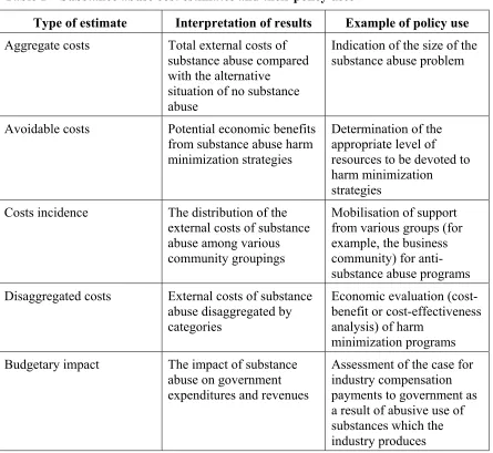
Table 1 – Substance abuse cost estimates and their policy uses

Type of estimate Interpretation of results Example of policy use Aggregate costs Total external costs of

substance abuse compared with the alternative

situation of no substance abuse

Indication of the size of the substance abuse problem

Avoidable costs Potential economic benefits from substance abuse harm minimization strategies

Determination of the appropriate level of resources to be devoted to harm minimization strategies

Costs incidence The distribution of the external costs of substance

Disaggregated costs External costs of substance abuse disaggregated by

Budgetary impact The impact of substance abuse on government expenditures and revenues

Assessment of the case for industry compensation payments to government as a result of abusive use of substances which the industry produces

The Guidelines provide considerable information on estimation of what, in Table 1 above, are referred to as aggregate costs. However, while aggregate cost estimates are extremely valuable for a number of purposes, as an indicator of the overall economic burden borne by the community as a result of substance abuse, they indicate neither the proportion of such aggregate costs which are potentially avoidable nor the nature of the programmes and policies best suited to achieve this cost avoidance. It was agreed by participants at workshops convened to develop the original guidelines that the next logical step in this area of research would be to proceed to the estimation of avoidable costs, which indicate the benefits potentially available to harm minimization programs.

In 2004, at the 46th Session of the Commission on Narcotic Drugs, the Government of Canada informed member states of its intention to launch an international initiative to develop guidelines for estimating avoidable costs of substance abuse. CCSA proposed the convening of a workshop to develop these guidelines. Health Canada agreed to

(11)

workshop attendees represented a wide range of academic disciplines, organizational backgrounds and countries. Two Australian economists, David Collins and Helen Lapsley, were commissioned to produce for the workshop a paper surveying the issues and problems involved in estimating the avoidable costs of substance abuse. Other papers dealing with specific areas of this research exercise were also commissioned for

presentation at the workshop. The survey paper and the other commissioned papers formed the basis for discussions at the workshop. The present avoidable cost guidelines represent a revised version of the original survey paper, very substantially rewritten and extended by its original authors in the light of the other commissioned papers and of discussions at the workshop. Where these new avoidable cost guidelines make extensive use of, or reference to, workshop papers or the comments of workshop participants, their authors are also formally acknowledged as joint authors of this report.

It is intended, as far as possible, to avoid overlap between this study and the previously published Guidelines_{for estimating the aggregate social costs of substance abuse. This} report concentrates on estimating the avoidable_{costs of substance abuse. It does not} attempt to discuss the wider issues involved in estimating the aggregate social costs of substance abuse except insofar as they are relevant to the estimation of avoidable costs. It is presumed that readers will already have some familiarity with the original aggregate cost Guidelines_.

However, international data on substance abuse have improved and, in some respects, the original Guidelines _{have the potential for further development. This is particularly true in} areas such as the epidemiological evidence about the effects of substance abuse and in the identification of drug-attributable crime. Accordingly, it is hoped that a third edition of the aggregate cost Guidelines _{will eventually be produced. In the meantime, this new} information needs to be acknowledged in the avoidable cost guidelines, even though technically it is more specifically related to the estimation of aggregate costs than to avoidable costs. Thus, the explanation of these developing areas is presented here but, in order to maintain the logical flow of this report, the information is presented in

appendices rather than in the main body of the report.

The aggregate cost Guidelines_{were produced by a group of authors all of whom had} practical experience in the estimation of the social costs of substance abuse. On the other hand, since the estimation of substance abuse avoidable_{costs is such a new area of} research, in which there is little published literature, few of the present authors have practical experience in this research area. With avoidable cost projects in various

(12)

1.2 The nature of avoidable costs

In estimating the aggregate costs of substance abuse, comparison must be made between the actual substance abuse situation and some alternative hypothetical situation, known as the counterfactual situation. This counterfactual, though often not specifically identified, is in most cost studies that of a situation of no past or present abuse of the substance(s) in question. Thus the counterfactual situation is implicitly one in which the community would bear no substance abuse costs. By comparing the actual situation with the counterfactual zero-abuse situation, the extra costs which that abuse imposes on the community can be calculated.

However, the hypothetical counterfactual situation is, as Single et al point out,

“hypothetical and not realizable under any circumstances. Estimates of the total costs of drug abuse comprise both avoidable and unavoidable costs. Unavoidable costs comprise the costs which are currently borne relating to drug abuse in the past, together with the costs incurred by the proportion of the population whose level of drug consumption will continue to involve costs. Avoidable costs are those costs which are amenable to public policy initiatives and behavioural changes.”

Thus, avoidable cost estimates provide an indication of the benefits potentially available to the community as a whole as a result of directing public resources to the prevention or reduction of substance abuse. They provide valuable economic information on the basis of which a more efficient allocation of productive resources could be achieved. It would be theoretically possible to have a situation in which, although aggregate substance abuse costs were high, avoidable costs were so low as not to justify public expenditures

designed to reduce abuse. In practice this is an unlikely scenario but it is one that might well be put forward, as an interpretation of aggregate cost estimates, by sectional interests opposed to the reduction of substance abuse. Although few estimates have been made of avoidable costs, those that have been made (see, for example, Collins and Lapsley, 1996 and 2002) indicate that avoidable costs represent in the order of fifty per cent of

aggregate costs. In the Australian context this level of avoidable costs provides

potentially very high rates of return on expenditures to reduce substance abuse (Collins and Lapsley, 1999 and 2004).

Avoidable cost estimates do not, on their own, indicate the rates of return which the community might achieve. Cost benefit analysis, or at the very least cost effectiveness analysis, is necessary to produce this type of information. However, without knowledge of the avoidable component of substance abuse costs it is difficult to undertake

meaningful cost-benefit analysis of prospective expenditures on prevention and/or treatment.

The process of estimating social costs involves estimating the relevant avoidable proportion of each of the cost categories and applying these proportions to each of the relevant aggregate cost estimates. Since not all substance abuse costs fall on the

(13)

1.3 Reasons for estimating avoidable costs

The original Guidelines_{laid out the four major purposes of guidelines for estimating the} aggregate social costs of substance abuse. These were:

1. Economic estimates are frequently used to argue that policies on alcohol, tobacco and other drugs should be given a high priority on the public policy agenda. 2. Cost estimates help to appropriately target specific problems and policies. 3. Economic cost studies help to identify information gaps, research needs and

desirable refinements to national statistical reporting systems.

4. The development of improved abuse cost estimates offers the potential to provide baseline measure to determine the efficacy of drug policies and programs.

Avoidable_{cost estimation can be justified on the same basis.}

1.3.1 Priority for substance abuse expenditures

In most countries, the allocation of public funds between competing programs is substantially influenced by pubic servants trained in economics or finance, who are looking to maximize the social rates of return on public expenditures. Accordingly, as part of the decision-making process, they utilize information on economic evaluation of the proposed expenditures. While aggregate cost estimates indicate the economic impact of substance abuse, they do not indicate what proportions of these costs are avoidable, and over what period of time. It is possible that some forms of substance abuse are much more susceptible to prevention measures than others, and so may yield higher gross benefits. Thus, avoidable cost estimates give a better indication of the potential benefits of anti-abuse programs and policies, though they still do not indicate the costs, and the rates of return, of appropriate programs. This issue is considered further below.

1.3.2 Appropriate targeting of specific problems and targets

Estimates of the avoidable costs of substance abuse, in conjunction with estimates of the aggregate costs, provide an extremely valuable information resource for policy analysis and design. This information is of two types:

• Cost estimation data. In the process of developing cost estimates, researchers generate virtually all the information necessary to value the benefits (that is, the reduction in social costs) of programs, once their physical outputs (in terms of , say, improved health outcomes, lower work absenteeism and reduced crime rates) have been determined:

(14)

Accordingly, avoidable cost estimation will facilitate both program analysis (through cost benefit analysis) and design of appropriate programs likely to yield the best achievable social rates of return.

1.3.3 Identification of information gaps and research needs

Systematic analysis of avoidable costs is likely to highlight information gaps which, when rectified, will facilitate improved policy design. This information will include answering such questions as:

• What substance abuse outcomes are potentially achievable?

• How best may these outcomes be achieved?

• Over what periods of time would these outcomes be achievable?

Since this information, in terms of both scientific analysis and policy analysis, will inevitably not be static, it will be necessary to review and update information concerning potential best practice on a regular basis.

1.3.4 Provision of baseline measures to determine the efficiency of drug policies and programs

Once policy makers have at their disposal measures of best practice substance abuse outcomes, they will be able much more efficiently to evaluate their existing anti-abuse policies and their allocation of public expenditures to and between anti-abuse programs. There is every reason to believe that the provision of avoidable cost estimates should lead to better policy design.

1.4 Reasons for producing avoidable cost guidelines

Almost no research work has been undertaken internationally to estimate the avoidable costs of substance abuse. There has, therefore, been little development of the necessary underlying theory, and data have not been systematically collected for this purpose. These research difficulties in this area are compounded by the fact that research skills from various disciplines are needed, including criminology, economics and

epidemiology.

The objective of guidelines in this area of research is to provide the theoretical and data framework for the estimation of the avoidable costs of substance abuse. Like the original

Guidelines_{, this publication is intended to provide a framework for analysis rather than a}

rigidly prescribed methodology.

It is hoped that these guidelines will encourage and facilitate the development in various countries of avoidable cost studies, leading to the provision of better information bases for the determination of national policies to counter substance abuse. Over time the underlying estimation methodologies will develop and improve. In addition,

(15)

2 Social costs

2.1 The types of social costs attributable to substance abuse

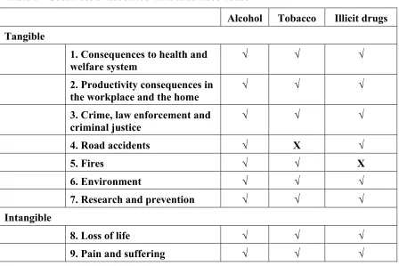
The aggregate cost Guidelines_(Singleet al_{, 2003) identify the main categories of} substance abuse costs. These are summarized in Table 2 below, which also indicates which categories of costs are relevant to which drugs.

Table 2 – Social costs associated with substance abuse

Alcohol Tobacco Illicit drugs Tangible

1. Consequences to health and welfare system

√ √ √

2. Productivity consequences in the workplace and the home

√ √ √

3. Crime, law enforcement and criminal justice

√ √ √

4. Road accidents √ X √

5. Fires √ √ X

6. Environment √ √ √

7. Research and prevention √ √ √

Intangible

8. Loss of life √ √ √

9. Pain and suffering √ √ √

Note: the symbol √ indicates relevant and the symbol X indicates not relevant

(16)

Tangible cost categories

1. Consequences to health and welfare system

1.1 Medical

2.1 Productivity consequences in the workplace

2.1.1 Reduction in paid workforce 2.1.2 Absenteeism

2.1.3 Reduced on-the-job productivity

2.2 Productivity consequences in the home

2.2.1 Reduction in unpaid workforce 2.2.2 Sickness

3. Crime, law enforcement and criminal justice

3.1 Law enforcement

3.7 Lost productivity of prisoners 3.8 Lost productivity of criminals 3.9 Insurance administration

4. Road accidents

4.1 Productivity in the workplace 4.2 Productivity in the home 4.3 Health care

(17)

It is probable that the basis for estimating the avoidable percentage of some cost

categories may be equally applicable to other cost categories. For example, the avoidable proportion of alcohol-attributable medical costs will probably also be applicable to alcohol-attributable hospital costs. However, for the purposes of systematic research, it is necessary to list all cost categories individually.

2.2 Health impacts of substance abuse

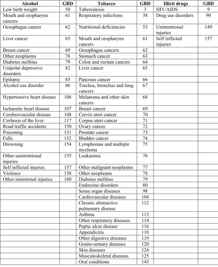
Table 3 lists all the conditions which a recent WHO international study (Ezzati et al, 2004) has concluded are causally and quantifiably linked to the abuse of alcohol, tobacco or illicit drugs. Quantifiability is very important since, if causal relationships are not quantifiable, it is not possible to estimate the costs of substance abuse or the potential benefits from appropriate anti-abuse policies. In practice, this list of quantifiable drug-attributable diseases has been steadily growing and other studies have produced different lists (see, for example, Appendix B which lists a substantially greater number of

(18)

Table 3 – Drug-attributable diseases for which the WHO has estimated attributable fractions

Alcohol GBD Tobacco GBD Illicit drugs GBD

Low birth weight 50 Tuberculosis 3 HIV/AIDS 9

Mouth and oropharynx cancers

61 Respiratory infections 38 Drug use disorders 90

Oesophagus cancer 62 Nutritional deficiencies 53 Unintentional injuries

149 Liver cancer 65 Mouth and oropharynx

cancers

61 Self inflicted injuries

157 Breast cancer 69 Oesophagus cancers 62

Other neoplasms 78 Stomach cancer 63

Diabetes mellitus 79 Colon and rectum cancers 64 Unipolar depressive

disorders

82 Liver cancer 65

Epilepsy 85 Pancreas cancer 66

Alcohol use disorder 86 Trachea, bronchus and lung cancers

67

Hypertensive heart disease 106 Melanoma and other skin cancers

68 Ischaemic heart disease 107 Breast cancer 69 Cerebrovascular disease 108 Cervix uteri cancer 70 Cirrhosis of the liver 117 Corpus uteri cancer 71 Road traffic accidents 150 Ovary cancer 72

Poisoning 151 Prostate cancer 73

Falls 152 Bladder cancer 74

Drowning 154 Lymphomas and multiple myeloma

75 Other unintentional

injuries

155 Leukaemia 76

Self inflicted injuries 157 Other malignant neoplasms 77

Violence 158 Other neoplasms 78

Other intentional injuries 160 Diabetes mellitus 79

Endocrine disorders 80

Other respiratory diseases 114

Peptic ulcer disease 116

(19)

3 Avoidable costs: the Feasible Minimum

3.1 Introduction

Where a particular event or medical condition can have more than a single cause it is necessary to have estimates of drug-attributable fractions. For instance, alcohol is not the only cause of road accidents nor is smoking the only cause of fire deaths. If the smoking-attributable fraction for lung cancer were estimated to be 0.84, it would then be known that 84 per cent of lung cancer cases were caused by smoking, the remaining 16 per cent of cases being attributable to other causes. In the absence of the relevant attributable fraction it is impossible to attribute the correct proportion of the total harm to substance abuse. In almost all cases the use of direct measures involves knowledge of attributable fractions.

This requirement can represent, in some areas of harm, a major difficulty in cost estimation. Calculation of attributable fractions (also known as aetiological fractions or attributable proportions) requires two fundamental pieces of information – the relative risk (measuring the causal relationship between exposure to the risk behaviour and the condition being studied) and prevalence (measuring the proportion of the relevant

population engaging in the risky activity). For some types of harm the relative risk can be assumed to be similar for genetically and economically similar populations. Applying the estimated prevalence for each population to the relevant relative risk will yield

attributable fractions which can be used to estimate harm in various populations (countries).

In practice, the attributable fractions in cost studies are derived from estimates of relative risks derived from research studies across a range of comparable countries. Generally, the calculations of the attributable fractions for all countries have in the past derived from studies conducted in a large set of countries with similarly high levels of economic development.

However, for some types of harm it would be quite unsafe to assume similar relative risks even in countries at similar levels of economic development. The most obvious type of harm in this context is crime where, for a range of cultural, social, legal and other reasons, relative risks can vary greatly even between countries with similarly high per capita incomes. A good example of the different rates of this type of harm is alcohol-attributable violence where experience varies greatly, even among Western European countries.

(20)

1. Even if substance abuse were to end immediately, many deaths and

hospitalizations (and other adverse consequences which lead to costs to the economy) would continue due to the lagged effects of past substance abuse.

2. When a risk factor (like substance abuse) causes a death or hospitalization, in a sense it may prevent another risk factor from causing a death or hospitalization. The obvious example is the fact that mortality is inevitable: everyone dies eventually from something or another, and if it is not due to substance abuse, it will be due to another cause.

3. There would necessarily be huge policy costs to end all substance abuse (in the unlikely event that this were possible), and it virtually impossible to estimate these costs as such policies have not even been identified, let alone costed.

The extent of the first problem is very difficult (and in practical terms, virtually impossible) to estimate. Given a set of assumptions concerning time intervals between different levels of use or risky behaviours and the onset of disease or death (information that is generally lacking), one could attempt to make estimates of lagged effects for some causes. But even if this could be done (which is highly doubtful), it would be limited to only a small subset of diagnoses. And in any case, the exercise would be of little use due to the second and third problems. Even with perfect information on the aetiology of substance-related diseases and accidents, researchers must still confront the other two problems.

It could be considered that the term substance abuse is misleading, because a significant portion of the burden attributable to drugs is caused by use only, i.e. by individuals who do not fall under the gold standard definitions of substance dependence or abuse (Rehm, 2003). For example, a road accident may be attributable to the intoxication (as defined by legislated maximum permissible blood alcohol content) of a driver who, nevertheless, would not fulfil any criterion of dependence or abuse in the International Classification of Diseases, Tenth Revision (ICD-10) (WHO, 1992-1994) or the Diagnostic and Statistical Manual of Mental Disorders, Fourth Edition (DSM-IV-R) (American Psychiatric

Association, 1994). Such alcohol use is often labelled as alcohol misuse. On the other hand, much alcohol use can, by any definition, clearly be categorised as abuse

Since social cost studies are essentially economic studies, they require a definition of substance abuse which is meaningful in economic terms. To economists, substance abuse exists when substance use involves the imposition of social costs additional to the

resource costs of the provision of that drug. Abuse occurs if society, including the substance user, incurs extra costs as a result of the drug use. Any use of illicit substances is deemed to be abuse since if use is deemed to be illegal it is clearly considered by society to be abuse

(21)

3.2 The concept of avoidability

The social costs of substance abuse worldwide are high (see, for example, Single et al, 1998; Harwood et al, 1998; Collins and Lapsley, 2002; and Andlin-Sobocki and Rehm, 2005). These costs are mainly related to the costs of health care, crime and law

enforcement, and losses in productivity. The substance abuse-related burden of disease is composed of the mortality and morbidity attributable to the abuse of alcohol, tobacco, and illegal drugs and is one of the main underlying components in substance abuse-related social costs. Knowing the overall attributable costs of substance abuse or the overall substance-abuse attributable disease burden has been found unsatisfactory, as it is not clear which proportion of the costs or the burden could in principle be changed. This changeable part has been labelled the avoidable cost or avoidable burden (WHO, 2002). Estimating avoidable burden is an important element in the process of estimating avoidable costs.

The first step in estimating avoidable burden is to conceptualise the attributable burden of disease; that is, the burden of a given disease in a given population that is identified as due to a specific exposure to a risk factor or multiple risk factors. Consequently, that portion of disease burden could, in principle, be reduced or eliminated if the causative exposure is reduced or eliminated. Attributable burden is conceptualized regardless of whether such a reduction is achievable in practice or not.

Based on the conceptualization of attributable burden, it is then possible to introduce the term avoidable burden of disease. The latter term denotes the proportion of disease burden that can be reduced by changing the current exposure distribution to an alternative, more favoured, exposure distribution. Clearly, the size of the avoidable burden caused by a given risk factor will always be smaller than or, at most, equal to the burden attributable to that risk factor. Little has been written on the problems of

estimating avoidable burdens/costs and so a discussion is presented below of a method to estimate avoidable burden specifically for substance use as a risk factor, with special emphasis on methodological problems and potential solutions.

3.3 Avoidability, optimality and zero tolerance

The avoidable burden/costs discussed here should be contrasted with the economist’s concept of the optimal level of substance abuse. Economists argue that the optimal level of drug consumption is reached when the incremental cost to the community as a whole of achieving a given reduction in consumption is exactly matched by the incremental benefit to the community of that reduction. If the incremental benefit is greater than the incremental cost, achieving optimality would require a further reduction in consumption. If the cost exceeds the benefit, then consumption has been reduced to sub-optimal levels.

The concepts of avoidability and optimality can lead to quite different outcomes. It is perfectly possible that optimal levels of consumption may not be achievable. For

(22)

to be optimal. In any event, there are likely in practice to be severe informational problems in determining optimal consumption levels. These guidelines concentrate on issues relating to the estimation of the avoidable costs of substance abuse, not the optimal levels of substance abuse.

Some public health advocates consider that the target for public health interventions should be a zero level of substance abuse. This might be called a zero tolerance approach. There are, for the purposes of these guidelines, problems with this approach from an economic perspective.

Economists would argue, as explained above, that in most situations the optimal outcome is not zero substance abuse but a level at which the additional costs of reducing abuse further are matched by the additional social benefits of that reduction. Even if zero substance abuse were achievable, in most instances the costs of achieving that outcome would exceed the benefits. In other words, the resources could be used more productively elsewhere.

In practice, zero abuse is not likely to be an achievable outcome. The concept of avoidable costs relates to what is achievable in the real world, not what would be desirable in an ideal world of unlimited resources.

3.4 Approaches to calculation of the Feasible Minimum

From an economic policy perspective, it is necessary to determine the maximum

quantifiable, measurable reduction in substance abuse costs which effective policies can be expected to achieve. The lowest achievable level of substance abuse can be termed the Feasible Minimum, and the four methodologies discussed here can be regarded as ways in which a Feasible Minimum can be calculated in order to provide policy objectives. Of course, such avoidable cost estimates assume that the calculation of total cost estimates will have already been undertaken. Various possible approaches exist for estimation of the Feasible Minimum.

One method of achieving an estimate of a Feasible Minimum is the use of the classic epidemiological approach, deriving the attributable burden from calculations of relative risk and the prevalence. From this calculation of the attributable burden, both past and future risk factor distributions can be estimated, which also provide data to enable the calculation of a Feasible Minimum. This approach can be modelled to demonstrate the difference between the attributable and the avoidable burden.

Armstrong applied this concept in his work on prevention, using a measure which he described as the “Arcadian normal” as his feasible minimum for preventable mortality for a range of conditions. Instead of using epidemiological data from which to calculate the feasible minimum, he used as a comparator the lowest recorded rate (e.g. of lung cancer) which had been achieved by a country which could be considered a reasonable

(23)

This concept does not in itself suggest that similar policies, regulations, and even health behaviours are necessarily appropriate nor transferable from the comparator country, but simply indicates what amount of burden reduction and costs have been able to be

achieved. A disaggregation of effective policies from a comparator country may be useful in developing economic evaluation studies, and provide guidance on resource distribution which could be made to different policy implementations.

Another possible approach to estimation of the Feasible Minimum is to use recently-published WHO data on drug-attributable fractions, morbidity and mortality. These data can be used to identify best performance among countries in sub-regions identified by the WHO as having common characteristics. This approach could be adopted for countries where insufficient domestic data are available. Although the only practical solution for many countries, it should be noted that this method is likely to be highly imprecise, given the multiple layering of assumption underlying the application of attributable fractions from one setting to another.

There may also be circumstances in which evidence about the known effectiveness of specific interventions may be used in avoidable proportions. This constitutes a fourth type of approach.

All four approaches are described in more detail below. Inevitably there are difficulties and complexities both in deriving the attributable fraction and then in calculating the proportion which is avoidable, which indicates the Feasible Minimum.

3.5 From the classical to the distributional approach in

epidemiology

Two different approaches to the epidemiology of risk factor attribution can be broadly distinguished: the classical epidemiological approach where, on the basis of a 2x2 table, disease risk can be estimated with respect to exposure and non-exposure of various populations to a single specific risk factor. Based on this categorically derived relative risk and the prevalence, the attributable burden can be derived, resulting in an estimate for a population who have already been exposed, i.e. focussing on the past. The main counterfactual scenario (Maldonado and Greenland, 2002) in this approach asks the question: “What would have happened if no exposure had occurred?”

More modern developments of epidemiology ask the question: “What would happen if risk factor distributions shifted to different counterfactual scenarios?” (Murray and

Lopez, 1999). The modern approach not only looks at distributional shifts at one time, but also takes the future time dimension into consideration, and thus is able to predict future developments.

(24)

policy. We will also consider potential interactions and competing risks between influencing factors.

(25)

3.5.1 An epidemiological model to estimate avoidable burden

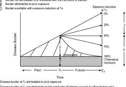
Figure 1 illustrates the conceptual model of the difference between attributable and avoidable burden, cited from the epidemiological model of Murray et al_(2003).

Figure 1 – A conceptual model of attributable and avoidable risk with increasing projected burden

Source: Murray, C.J.; Ezzati, M.; Lopez, A.D.; Rodgers, A.; and VanderHoorn, S (2003). “Comparative quantification of health risks conceptual framework and methodological issues”,

Population Health Metrics, 1(1): 1-20.

Consider the disease burden at time T0 (that portion which is attributable to prior

exposure), denoted by the letter a_{in Figure 1. This is all the burden of disease which can} be attributed to prior exposure of the risk factor under consideration before T0.

Burden not attributable to or avoidable with the risk f actor of interest Burden attributable to prior exposure

Burden avoidable with exposure reduction at To

a Disease burden at Toat tributable to prior expos ure

b Disease burden at Tonot attributable to t he risk f actor of interest (caused by other factors only). The burden not attribut able to the risk f actor of interest (grey area) may be decreasing, constant or increasing over time. The constant case is shown in t he figure.

c Disease burden avoidable at Tx with a 50% exposure reduction at To. d Remaining disease burden at Txaf ter a 50% reduction in risk fact or exposure

(26)

In the example, a general situation is given where the background burden, i.e. the burden due to other factors except the risk factor under consideration, is constant over time. This background burden is denoted by the letter b_{at time T}₀_{and, because it is constant over} time in this specific example, the burden is the same size at all time points. Of course, in other situations the burden attributable to other factors than the risk factor under

consideration may fluctuate.

The burden attributable to the risk factor under consideration in the example is increasing constantly over time until time T0. Then different scenarios are shown. Let us discuss three of them. If nothing (e.g. intervention, changes in cultural acceptance) happens at time T0, the attributable burden continues to increase linearly. On the other hand, if the exposure is reduced completely, then the attributable burden is decreasing until time Tx, when it reaches zero.

Consider tobacco use as an example in a society where prevalence rates have been increasing and would continue to increase without any intervention. If some drastic intervention could reduce smoking completely at a certain time point, smoking-related disease burden would not be zero the moment thereafter. Instead, some burden of disease would persist, e.g. burden of disease due to existing tobacco-related lung cancer, and some people may even develop new lung cancer based on their past exposure.

Now consider a reduction of exposure to the risk factor by 50 per cent at time T0. In the example, such a reduction would mean that a constant attributable burden would result. This burden is, of course, a mixture of the impact of past exposure (i.e. prior to T0) plus the impact of the exposure after T0.

Three main components have to be known to estimate this model. They are:

1. The relationship between exposure (i.e. the risk factor under consideration) and disease burden (attributable risk) and its temporal trend

2. The amount of burden caused by other factors than the risk factor under consideration and the temporal stability of this burden.

3. The specific trajectory of burden reduction after exposure reduction

Methods to estimate the relationship between a certain exposure distribution and disease burden are well established (e.g., odds ratios, relative risks; see Rothman and Greenland, 1998). Similarly, methods to estimate the proportion of burden attributable to the

distribution of a certain risk factor were developed some decades ago and were first described by Miettinen (1972) in the early 1970s and Walter a little while later (Walter, 1976; 1980). They have since been used to generate estimates of the attributable burden for substance use and other risk factors around the world (Ezzati and Lopez, 2000). The key concept used herewith is that of an attributable fraction (AF; also called the

(27)

Below are the two formulas for the case of continuous exposure levels and the discrete case, both of which are fully developed and described elsewhere (Walter, 1976; 1980; Eide and Heuch, 2001; Murray et al., 2003).

The contribution of a risk factor to disease can be estimated by comparing the burden due to the observed exposure distribution in a population with that from another distribution

(rather than a single reference level such as non-exposed) as described by the generalized equation shown as Equation 1.

Equation 1

where PIF is the “potential impact fraction”, a generalized form of the attributable fraction; RR(x) is the relative risk at exposure level x, P(x) is the population distribution of exposure, P' (x) is the counterfactual distribution of exposure, and m the maximum exposure level. As Murray et al. (2003) have noted, this formula can be further

generalized to deal with a situation, where the relative risks change in the counterfactual scenario.

The corresponding relationship when exposure is described as a discrete variable with k levels is given by Equation 2.

Equation 2:

i: exposure level category

RRi: relative risk at exposure level i

Pi: prevalence of the ith category of exposure

The concept of attributable fraction (or the generalized form of PIF), as defined here, can only describe a snapshot at a specific time. Attributable fractions without including a time dimension are not able to characterize those cases whose occurrence would have been delayed or in part prevented due to exposure reduction (see Greenland and Robins, 1988). As a remedy, Greenland and Robins (1998) recommend the use of aetiologic fractions with a time dimension to account for this shortcoming. Time-based measures are

(28)

The theoretical minimum risk (see Figure 1) is trickier to define than the exposure-burden relationship. Theoretical minimum risk denotes the exposure distribution that would result in the lowest population burden, irrespective of whether such a distribution is currently attainable in practice (Murray and Lopez, 1999). In the example it was set at zero attributable burden, but this is not necessarily always the case. Consider alcohol, and assume only one relevant exposure dimension in disease aetiology (see below for a discussion of volume and patterns of drinking as a two-dimensional exposure

association), such as average volume of drinking. Minimal risk then occurs at zero (i.e. no drinking at all) for most related diseases such as cancer or traffic injury, but not for some whose risk actually decreases at exposures greater than zero e.g. heart disease (Rehm et al_{, 2003a; Rehm}et al_{, 2003b; Rehm}et al_{, 2004). For composite outcome}

measures, e.g. all-cause mortality, there is also reason to believe that the level of the exposure associated with minimum burden is greater than zero (i.e. some level of drinking) (Rehm et al_{, 2001; Gmel}et al_{, 2003). The exact value of exposure associated}

with the minimal burden will depend on the composite measure used, and the disease distribution in the country or region examined. Thus, the theoretical minimum risk will fluctuate across cultures.

A theoretical minimum risk with an exposure greater than zero has interesting

implications. For alcohol in the above example it means that, even if drinking occurs at the theoretical minimum, there will be some attributable disease burden. For instance, in a society with relatively large coronary burden and assuming a theoretical minimum risk for the population occurring at approximately 1 drink/day, there will be disease burden associated with such an exposure level of moderate drinking, e.g., for certain

gastrointestinal diseases (Taylor et al_{, 2005) or accidents (Rehm and Gmel, 2003).}

The above example is hypothetical for several reasons:

a) It assumes all people having the same exposure level (1 drink/day for all people) rather than a distribution of exposure, known to exist for all populations drinking alcohol. (Skog, 1985). Note that the above statement only refers to the existence of a distribution and does not specify the exact shape of it (e.g., lognormal vs. Poisson).

b) It completely disregards the fact that alcohol has at least two dimensions relevant for disease, average volume of alcohol consumption and patterns of drinking (Rehm et al_{, 2003a).}

c) There is no known intervention, which would result in the above-mentioned distribution of 1 drink/day for all (Babor et al_{., 2003; Room}et al_{., 2005).}

In more general terms, the following points can be made:

a) We should always model shifts in risk factor distributions when estimating avoidable burden of disease.

(29)

c) We need other counterfactual scenarios in addition to the theoretical minimum risk, when estimating avoidable burden of disease. The question will be where to obtain the counterfactual scenarios from.

The trajectory of the burden reduction after changes in exposure is also difficult to define, not only because it should incorporate changes of exposure reduction as well, but because it also has to make estimates for the change of relative risk over time of several disease outcomes, potentially both acute (e.g., alcohol and deaths from drinking and driving) and chronic (e.g. alcohol and chronic pancreatitis). For instance, after a change of smoking status to abstinence, we have to know the relative risk of an ex-smoker after one year after abstaining, two years after abstaining, three year after abstaining, and so on. For acute outcomes, the problem is much easier. Once the prevalence of alcohol, tobacco or illicit drugs is reduced, all the acute outcomes (e.g. injuries) are reduced accordingly. To give an example: while drinking over the past years does affect the cancer risk of people today, even if they started abstaining in between, it does not affect the traffic accident risk.

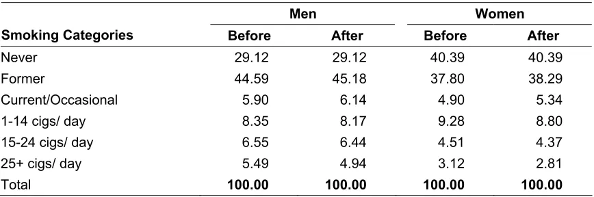
3.5.2 An example: shifting the smoking distribution in Canada by 10 per cent

(30)

Table 4 – Resulting prevalence of tobacco smoking in per cent after a -10 per cent shift in exposure distribution in Canada 2003, by gender

Men Women

Smoking Categories Before After Before After

Never 29.12 29.12 40.39 40.39 Former 44.59 45.18 37.80 38.29 Current/Occasional 5.90 6.14 4.90 5.34

1-14 cigs/ day 8.35 8.17 9.28 8.80 15-24 cigs/ day 6.55 6.44 4.51 4.37 25+ cigs/ day 5.49 4.94 3.12 2.81

Total 100.00 100.00 100.00 100.00

Table 4 shows the gender-specific shift in prevalence of smoking for different categories before and after a 10 per cent decrease in each exposure prevalence category as described above. Overall, smoking prevalence decreased by 2.2 per cent on both genders. The impact this shift distribution had on tobacco-related disease-specific mortality was modelled based on the mortality data for 2002. The baseline scenario was taken from the second Canadian study on social costs of substance abuse where tobacco-related

attributable burden was modelled gender, age and disease specific with a counterfactual scenario of zero smoking as the level denoting minimal risk (Baliunas et al., 2005). To estimate avoidable burden, the shift in prevalence was again modelled specifically by gender, age and disease, resulting in the reduction of smoking-related mortality

summarized in Table 5. The relative risk to denote the relationships between category of exposure and outcome were taken from meta-analyses (for details see Baliunas et al., 2005). More than 20 different disease categories had to be modelled in order to arrive at Table 5.

Table 5 – Impact of exposure shift of -10 per cent in exposure to tobacco smoking on disease-specific, tobacco-attributable mortality in Canada, 2002 (number of deaths)

Lung

(31)

A distributional shift of 10 per cent in the exposure level to tobacco smoke resulted in 938 fewer tobacco-attributable deaths, 2.1 per cent less than before the shift. The largest absolute differences before and after were seen for lung cancer and cardiovascular diseases, and also for deaths due to lung cancer and ischemic heart disease attributable to passive smoking. However, relative differences were most pronounced for the acute outcomes.

The above example illustrates the possibilities of modelling avoidable burden using the above specified framework based. It also illustrates which points still have to be

improved. First, smoking-related attributable burden is still modelled in a way using current levels of smoking as an indicator of cumulated past exposure. While this

procedure is usual in the literature and the basis of the most-used software for calculation smoking-attributable mortality, it clearly introduces measurement error, which may increase, as smoking behaviour across the lifespan does not seem to be as stable as it used to be. Second, the distributional shift is somewhat arbitrary in two ways: it is not clear why a 10 per cent shift should be the basis for avoidable burden, nor are the actual shifts in prevalence empirically based. For instance, in interventions underlying reductions in smoking prevalence such as taxation, different shifts in smoking prevalence distributions might be seen (e.g. changing from the highest smoking level into abstention). Finally, it is again a snapshot picture, depicting one change without incorporating the time dimension.

However, to generally select which shifts should be modelled, and how realistic they are, it may still be helpful to look at similar countries or historical trends as comparators. Thus, one would first screen plausible developments based on historical trends or the distribution in other countries, and then model shifts in risk factor distributions and subsequently the avoidable burden associated with this shift. For the Canadian example below, one would look at the distributional changes resulting from intervention packages being used in countries or regions similar to Canada and model avoidable burden

accordingly.

3.6 The Arcadian normal

A second type of approach to estimating the Feasible Minimum is by estimating what has become known as the Arcadian normal_{. Pioneering work in this area was done by}

Armstrong (1990). His work was expressed in terms of preventable mortality and

morbidity but it is reasonable to extend the concepts embodied in his work to other costs such as the property costs resulting from drug-attributable crime or smoking-attributable fires. He talks of assuming “the existence of some level of disease that might reasonably be achieved if only we knew all that might reasonably be known about the causes of the disease in question and could apply them in practical programmes in the community. There is no simple way of identifying this level of disease but it may be assumed to be less than the lowest level of disease that obtains in some group of genetically similar populations”. Armstrong terms this level of disease the ‘Arcadian normal’ “because it represents the nearest approach that we can make to harmony between humankind and its environment. Arcadia, in ancient Greece, was a region renowned for the contented

(32)

Armstrong’s approach is to compare the most recently available age standardised mortality rates for a range of causes in a group of countries with genetically similar populations and with similar living standards. He takes the Arcadian normal to be the lowest age-standardised mortality rate for each cause of death in the 20 European countries he studied and from these he estimates the proportions of potentially preventable mortality in Australia. His results are presented in Table 6 below.

Table 6 – Estimates of potentially preventable mortality in Australia

Cause of death

Circulatory diseases 410 France 265 35.4

Ischaemic heart disease 231 France 76 67.1

Cerebrovascular disease 95.6 Canada 57.5 39.8

Respiratory diseases 64.7 Austria 42.5 34.3

Chronic bronchitis,

Injury and poisoning 50.4 England and Wales

34.3 31.9

Road crashes 17.9 England and

Wales

8.8 50.8

Suicide 11.8 Greece 3.9 66.9

* Age-standardised mortality rate per 100,000 of the population Source: Armstrong (1990)

Note that Armstrong’s table, as presented in his 1990 paper, is reproduced above solely to illustrate the concept of the Arcadian normal. It is not suggested that the actual estimates of the normals presented in that paper should be used in future studies. Clearly new information has become available in the years since Armstrong’s important paper was published.

(33)

America, Western Europe, Oceania). Even though the Arcadian normal expressed in terms of smoking prevalence may be 15 per cent now, it will probably be much lower in another decade. This calls to question the whole idea of using historical examples as an absolute standard. Fifty years from now the Arcadian normal for smoking may only be 5 per cent or 10 per cent. Two hundred years ago it would have been close to zero. Arcadian normals are a reasonable approximation for a given place and time period only.

Table 6 above indicates that the more disaggregated is the information on mortality and morbidity, the more likely it is to lead to accurate estimates of the normal. As an

illustration, Table 6 shows that the derivation of individual Arcadian normals for specific types of cancer would be more accurate in producing percentages preventable than simply applying the across-the-board figure for all cancers. This is especially true when dealing with drug attributable diseases, since the drug attribution factors for different diseases will vary widely (and will, in many cases, be zero).

In principle it would be desirable to have individual Arcadian normals for every drug-attributable condition, although this is, in practice, unlikely to be achievable.

In estimating the Arcadian normal, direct or indirect (proxy) measures can be used. Direct measures are physical or financial measures which relate directly to the costs attributable to substance abuse. For example, alcohol-attributable road accidents or smoking-attributable fire deaths are direct measures of harm resulting from substance abuse. Economists can then translate these physical measures into financial costs. However, for almost every harm linked to substance abuse there are multiple causes. Alcohol is not the only cause of road accidents nor is smoking the only cause of fire deaths. Where a particular event or medical condition can have more than a single cause it is necessary to have estimates of substance-attributable fractions. For example, if the smoking-substance-attributable fraction for lung cancer were estimated to be 0.84, it would then be known that 84 per cent of lung cancer cases were caused by smoking, the remaining 16 per cent of cases being attributable to other causes. In the absence of the relevant attributable fraction it will be impossible to attribute the correct proportion of the total harm to substance abuse. In almost all cases the use of direct measures involves knowledge of attributable fractions.

This requirement can represent, in some areas of harm, a major obstacle to the use of direct measures. As indicated above, calculation of attributable fractions requires two fundamental pieces of information – the relative risk and prevalence. For some types of harm the relative risk can be assumed to be similar for genetically and economically similar populations. Applying the estimated prevalence for each population to the relevant relative risk will yield attributable fractions which can be used to estimate harm in the various populations (countries).

Nevertheless, there exist some significant issues with the Arcadian normal which must be acknowledged when making these types of calculations

(34)

• Second, the theoretical minimum needed in our framework is for burden of disease across different diseases, not for an individual disease category. Summing up across disease categories has the additional problem that the Arcadian normal will stem from different countries (in Armstrong’s analysis, France for CHD, Austria for infectious disease, Sweden for digestive disease etc.) which means different burdens from factors other than the exposure under consideration have to be taken into account.

• Third, countries may be so different with respect to other factors that they may not be comparable as regards achievable disease reduction. There might also be other reasons, such as cultural differences (e.g. Muslim countries with very low alcohol consumption), which explain different exposure levels, and such “feasible” exposure levels might not be really feasibly achieved in other countries.

An additional issue is that the Arcadian normal procedure should require appropriate adjustment for long-term global trends, such as the trend away from smoking. Smoking rates are declining significantly across the board in many regions (e.g., North America, Western Europe, Oceania). Even though the Arcadian normal expressed in terms of smoking prevalence may be 15 per cent now, it will probably be much lower in another decade. This calls to question the whole idea of using historical examples as an absolute standard. Fifty years from now the Arcadian normal for smoking may only be 5 per cent or 10 per cent. Two hundred years ago it would have been close to zero. Arcadian normals are a reasonable approximation for a given place and time period only.

Armstrong’s Arcadian normal will not work for the model proposed above because this model needs instead an exposure-specific feasible minimum of disease burden. The concept of the Arcadian normal could, however, be transferred to exposure and could define feasible exposure changes based on the minimum of exposure distributions in similar societies achieved by intervention. It would thus introduce a Feasible Minimum (Murray and Lopez, 1999) – defined as an exposure distribution that has already been achieved in comparable societies. This possibility is developed in Section 3.7 below.

Using a Feasible Minimum will result in more practically achievable solutions and thus less avoidable burden than if using a purely theoretical minimum. It would also be possible to estimate pathways towards the avoidable burden in hypothetical scenarios based on changes to current risk factor exposure, making this a powerful statistical tool for policy and intervention development. However, we would still have to deal with problems of comparability between countries.

3.7 Exposure-based comparators

(35)

The recent publication by the World Health Organisation of Comparative Quantification of Health Risks (Ezzati et al, 2004) has produced a significant improvement in the

availability of information on the relationships between, on the one hand, substance abuse and, on the other, mortality and morbidity. The Annex to Ezzati et al (op cit) provides population attributable fractions for a wide range of substance abuse-disease

relationships, classified by age, sex and sub-region. Also provided, cross-classified according to the same variables, are attributable fractions for years of life lost to

premature mortality (YLL) and overall disease burden as measured by disability adjusted life years (DALYs). Fuller details of this information are provided in Appendix A below.

As indicated above, the calculation of attributable fractions requires information on both relative risk and prevalence. On the assumption that relative risk is the same for all countries within a WHO-defined region, variations in prevalence within the sub-region could be considered as proxies for variations in attributable fractions (for

definitions of the sub-regions see Appendix A). The higher the prevalence rate, the higher will be the attributable fraction. By comparing the prevalence rate in the country under study with the lowest prevalence rate of all countries in the sub-region, an estimate can be made of the percentage of burden, and therefore of costs, that is avoidable. This

approach, though simplified, is still consistent with our recommended concentration on

exposure as an indication of the Arcadian normal, rather than outcomes.

A considerable amount of information on the international prevalence of drug use is available from WHO sources, particularly the WHO Statistical Information Service (WHOSIS) and the Organisation’s Global Alcohol Database, Global Information System of Tobacco Control and Tobacco Atlas (Mackay and Eriksen, 2002).

Consider the example of smoking prevalence in WHO sub-region AMR-D, defined in Ezzati et al (2004) as consisting of Bolivia, Ecuador, Guatemala, Haiti, Nicaragua and Peru. Table 7 below presents adult smoking percentages, classified by sex, for the countries in this sub-region.

Table 7 – Adult smoking prevalence, WHO sub-region AMR-D

Prevalence rate Country

Male (per cent)

Female (per cent)

Total (per cent)

Bolivia 42.7 18.1 30.4

Ecuador 45.5 17.4 31.5

Guatemala 37.8 17.7 27.8

Haiti 10.7 8.6 9.7

Nicaragua n.a. n.a. n.a.

Peru 41.5 15.7 28.6