An Introduction to Environmental Biophysics

Gaylon S. Campbell

John

M.

Norman

An Introduction to

Environmental

Biophysics

Second Edition

With 8 1 Illustrations

950 NE Nelson Ct. Pullman, WA 99163 USA

College of Agricultural and Life Sciences Soils Madison, WI 53705 USA

Library of Congress Cataloging-in-Publication Data Campbell, Gaylon S.

Introduction to environmental biophysics/G. S. Campbell, J. M. Norman.

--

2nd ed.

p. cm.

Includes bibliographical references and index. ISBN 0-387-94937-2 (softcover)

1. Biophysics. 2. Ecology. I. Norman, John M. 11. Title. CH505.C34 1998

571.4-dc2 1 97-15706

Printed on acid-free paper.

O 1998 Springer-Verlag New York, Inc.

All rights resewed. This work may not be translated or copied in whole or in part without the written permission of the publisher (Springer-Verlag New York, Inc., 175 Fifth Avenue, New York, NY 10010, USA), except for brief excerpts in connection with reviews or scholarly analy- sis. Use in connection with any form of information storage and retrieval, electronic adaptation, computer software, or by similar or dissimilar methodology now known or hereafter developed is forbidden.

The use of general descriptive names, trade names, trademarks, etc., in this publication, even if the former are not especially identified, is not to be taken as a sign that such names, as under- stood by the Trade Marks and Merchandise Marks Act, may accordingly be used freely by any- one.

Production coordinated by Black Hole Publishing Services, Berkeley, CA, and managed by Bill Imbornoni; manufacturing supervised by Johanna Tschebull.

Typset by Bartlett Press, Marietta, GA.

Printed and bound by Edwards Brothers, Inc., Ann Arbor, MI. Printed in the United States of America.

9 8 7 6 5 4 3 2 (Corrected second printing, 2000)

ISBN 0-387-94937-2 SPIN 10768147

Springer-Verlag New York Berlin Heidelberg

Preface to the

Second Edition

The objectives of the first edition of "An Introduction to Environmental Biophysics" were "to describe the physical microenvironment in which living organisms reside" and "to present a simplified discussion of heat and mass transfer models and apply them to exchange processes between organisms and their surroundings." These remain the objectives of this edition. This book is used as a text in courses taught at Washington State University and University of Wisconsin and the new edition incorporates knowledge gained through teaching this subject over the past 20 years. Suggestions of colleagues and students have been incorporated, and all of the material has been revised to reflect changes and trends in the science. Those familiar with the first edition will note that the order of pre- sentation is changed somewhat. We now start by describing the physical environment of living organisms (temperature, moisture, wind) and then consider the physics of heat and mass transport between organisms and their surroundings. Radiative transport is treated later in this edition, and is covered in two chapters, rather than one, as in the first edition. Since remote sensing is playing an increasingly important role in environmen- tal biophysics, we have included material on this important topic

as

well. As with the first edition, the h a 1 chapters are applications of previously described principles to animal and plant systems.

Many of the students who take our courses come from the biolog- ical sciences where mathematical skills are often less developed than in physics and engineering.

Our

approach, which starts with more de- scriptive topics, and progresses to topics that are more mathematically demanding, appears to meet the needs of students with this type of back- ground. Since we expect students to develop the mathematical skills necessary to solve problems in mass and energy exchange, we have added many example problems, and have also provided additional problems for students to work at the end of chapters.

are used. Also, molar units are becoming widely accepted in biological science disciplines for excellent scientific reasons (e.g., photosynthetic light reactions clearly are driven by photons of light and molar units are required to describe this process.) A coherent view of the connectedness of biological organisms and their environment is facilitated by a uniform system of units. A third reason for using molar units comes from the fact that, when difisive conductances are expressed in molar units, the numerical values are virtually independent of temperature and pressure. Temperature and pressure effects are large enough in the old system to require adjustments for changes in temperature and pressure. These tem- perature and pressure effects were not explicitly acknowledged in the first edition, making that approach look simpler; but students who delved more deeply into the problem found that, to do the calculations correctly, a lot of additional work was required. A fourth consideration is that use of a molar unit immediately raises the question "moles of what?" The dependence of the numerical value of conductance on the quantity that is diffusing is more obvious than when units of m/s are used. This helps students to avoid using a diffusive conductance for water vapor when estimating a flux of carbon dioxide, which would result in a 60 percent error in the calculation. We have found that students adapt readily to the consistent use of molar units because of the simpler equations and explicit dependencies on environmental factors. The only disadvantage to using molar units is the temporary effort required by those familiar with other units to become familiar with "typical values" in molar units.

A second convention in this book that is somewhat different from the first edition is the predominant use of conductance rather that resistance. Whether one uses resistance or conductance is a matter of preference, but predominant use of one throughout a book is desirable to avoid con- fusion. We chose conductance because it is directly proportional to flux, which aids in the development of an intuitive understanding of trans- port processes in complex systems such as plant canopies. This avoids some confusion, such as the common error of averaging leaf resistances to obtain a canopy resistance. Resistances are discussed and occasion- ally used, but generally to avoid unnecessarily complicated equations in special cases.

Preface to the Second Edition vii

are the best way to resolve this problem so that misinterpretations do not occur. For those interested only in exchanges with flat leaves, the develop- ment in this book may seem somewhat more complicated. However, "flat leaf' versions of the equations are easy to write and when interest extends to nonilat objects this analysis will be fully appreciated. When extending energy budgets to canopies we suggest herni-surface area, which is one- half the surface area. For canopies of flat leaves, the hemi-surface area index is identical to the traditional leaf area index; however for canopies of nonflat leaves, such as conifer needles, the hemi-surface area index is unambiguous while "projected" leaf area index depends on many factors that often are not adequately described.

One convention that remains the same as the first edition is the use of J k g for water potential. Although pressure units (kPa or MPa) have become popular in the plant sciences, potential is an energy per unit mass and the J/kg unit is more fundamental and preferred. Fortunately, J k g and kPa have the same numerical value so conversions are simple.

As with the previous edition, many people contributed substantially to this book. Students in our classes, as well as colleagues, suggested better ways of presenting material. Several publishers gave permission to use previously published materials. Marcello Donatelli checked the manuscript for errors and prepared the manuscript and figures to be sent to the publisher. The staff at Springer-Verlag were patient and supportive through the inevitable delays that come with full schedules. We are also grateful to our wives and families for their help and encouragement in finishing this project. Finally, we would like to acknowIedge the contri- butions of the late Champ B. Tanner. Most of the material in this book was taught and worked on in some form by Champ during his years of teach- ing and research at University of Wisconsin. Both of us have been deeply influenced by his teaching and his example. We dedicate this edition to him.

G. S. Campbell J. M. Norman

Preface to the

First Edition

The study of environmental biophysics probably began earlier in man's history than that of any other science. The study of organism- environment interaction provided a key to survival and progress. Systematic study of the science and recording of experimental results goes back many hundreds of years. Benjamin Franklin, the early American statesmen, inventor, printer, and scientist studied conduction, evaporation, and radiation. One of his observation is as follows:

My desk on which I now write, and the lock of my desk, are both exposed to the same temperature of the air, and have therefore the same degree of heat or cold; yet if I lay my hand successively on the wood and on the metal, the latter feels much the coldest, not that it is really so, but being a better conductor, it more readily than the wood takes away and draws into itself the fire that was in my skin.

'

Progress in environmental biophysics, since the observation of Franklin and others, has been mainly in two areas: use of mathematical models to quantify rates of heat and mass transfer and use of the continuity equation that has led to energy budget analyses. In quantification of heat- and mass-transfer rates, environmental biophysicists have followed the lead of physics and engineering. There, theoretical and empirical models have been derived that can be applied to many of the transport problems encountered by the design engineer. The same models were applied to transport processes between living organisms and their surroundings.

This book is written with two objectives in mind. The first is to de- scribe the physical micro environment in which living organisms reside. The second is to present a simplified discussion of heat- and mass-transfer models and apply them to exchange processes between organisms and their surroundings. One might consider this a sort of engineering approach to environmental biology, since the intent to teach the student to calcu- late actual transfer rates, rather than just study the principles involved.

- - -

Numerical examples are presented to illustrate many of the principles, and are given at the end of each chapter to help the student develop skills using the equations. Working of problems should be considered as es- sential to gaining an understanding of modern environmental biophysics as it is to any course in physics or engineering. The last four chapters of the book attempt to apply physical principles to exchange processes of living organisms, the intent was to indicate approaches that either could be or have been used to solve particular problems. The presentation was not intended to be exhaustive, and in many cases, assumptions made will severely limit the applicability of the solutions. It is hoped that the reader will find these examples helpful but will use the principles presented in the first part of the book to develop his own approaches to problems, using assumptions that fit the particular problem of interest.

Literature citation have been given at the end of each chapter to indicate sources of additional material and possibilities for further reading. Again, the citations were not meant to be exhaustive.

Many people contributed substantially to this book. I first became inter- ested in environmental biophysics while working as an undergraduate in the laboratory of the late Sterling Taylor. Walter Gardner has contributed substantially to my understanding of the subject through comments and discussion, and provided editorial assistance on early chapters of the book. Marcel Fuchs taught me about light penetration in plant canopies, provided much helpful discussion on other aspects of the book, and read and commented on the entire manuscript. James King read Chapters 7

and 8 and made useful criticisms which helped the presentation. He and his students in zoology have been most helpful in providing discussion and questions which led to much of the material presented in Chapter

7. Students in my Environmental Biophysics classes have offered many helpful criticisms to make the presentation less ambiguous and, I hope, more understandable. Several authors and publishers gave permission to use figures, Karen Ricketts typed all versions of the manuscript, and my wife, Judy, edited the entire manuscript and offered the help and encour- agement necessary to bring this project to completion. To all of these people, I am most grateful.

Contents

Preface to the Second Edition

Preface to the First Edition

List of Symbols

Chapter 1 Introduction

1.1 Microenvironments 1.2 Energy Exchange

1.3 Mass and Momentum Transport 1.4 Conservation of Energy and Mass 1.5 Continuity in the Biosphere 1.6 Models, Heterogeneity, and Scale 1.7 Applications

1.8 Units References Problems

Chapter 2 Temperature

2.1 Typical Behavior of Atmospheric and Soil Temperature 2.2 Random Temperature Variation

2.3 Modeling Vertical Variation in Air Temperature 2.4 Modeling Temporal Variation in Air Temperature 2.5 Soil Temperature Changes with Depth and Time 2.6 Temperature and Biological Development 2.7 Thermal Time

2.8 Calculating Thermal Time from Weather Data

2.9 Temperature Extremes and the Computation of Thermal Time

2.10 Normalization of Thermal Time

2.1 1 Thermal Time in Relation To Other Environmental Variables

References Problems

Chapter 3 Water Vapor and Other Gases 37

3.1 Specifying Gas Concentration 3 8

3.2 Water Vapor: Saturation Conditions 40

3.3 Condition of Partial Saturation 42

3.4 Spatial and Temporal Variation of Atmospheric Water

Vapor 47

3.5 Estimating the Vapor Concentration in Air 49

References 50

Problems 50

Chapter 4 Liquid Water in Organisms and their Environment 53 4.1 Water Potential and Water Content

4.2 Water Potentials in Organisms and their Surroundings 4.3 Relation of Liquid- to Gas-Phase Water

References Problems

Chapter 5 Wind

5.1 Characteristics of Atmospheric Twbulence 5.2 Wind as a Vector

5.3 Modeling the Variation in Wind Speed 5.4 Finding the Zero Plane Displacement and the

Roughness Length

5.5 Wind Within Crop Canopies References

Problems

Chapter 6 Heat and Mass Transport 6.1 Molar Fluxes

6.2 Integration of the Transport Equations 6.3 Resistances and Conductances 6.4 Resistors and Conductors in Series 6.5 Resistors in Parallel

6.6 Calculation of Fluxes Problems

Chapter 7 Conductances for Heat and Mass Transfer 7.1 Conductances for Molecular Diffusion

7.2 Molecular Diffusivities

7.3 Diffusive Conductance of the Integument 7.4 Turbulent Transport

7.5 Fetch and Buoyancy

7.6 Conductance of the Atmospheric Surface Layer 7.7 Conductances for Heat and Mass Transfer in

Laminar Forced Convection

Contents xiii

7.10 Combined Forced and Free Convection 7.1 1 Conductance Ratios

7.12 Determining the Characteristic Dimension of an Object 7.13 Free Stream Turbulence

Summary of Formulae for Conductance References

Problems

Chapter 8 Heat Flow in the Soil

8.1 Heat Flow and Storage in Soil

8.2 Thermal Properties of Soils: Volumetric Heat Capacity 8.3 Thermal Properties of Soils: Thermal Conductivity 8.4 Thermal Diffusivity and Admittance of Soils 8.5 Heat Transfer from Animals to a Substrate

References Problems

Chapter 9 Water Flow in Soil

9.1 The Hydraulic Conductivity 9.2 Infiltration of Water into Soil 9.3 Redistribution of Water in Soil 9.4 Evaporation from the Soil Surface 9.5 Transpiration and Plant Water Uptake 9.6 The Water Balance

References Problems

Chapter 10 Radiation Basics

10.1 The Electromagnetic Spectrum 10.2 Blackbody Radiation

10.3 Definitions 10.4 The Cosine Law

10.5 Attenuation of Radiation

10.6 Spectral Distribution of Blackbody Radiation 10.7 Spectral Distribution of Solar and Thermal Radiation 10.8 Radiant Emittance

References Problems

Chapter 11 Radiation Fluxes in Natural Environments

1 1.1 Sun Angles and Daylength

1 1.2 Estimating Direct and Diffuse Short-wave Irradiance 1 1.3 Solar Radiation under Clouds

1 1.4 Radiation Balance

1 1.6 View Factors References Problems

Chapter 12 Animals and their Environment

12.1 The Energy Budget Concept 12.2 Metabolism

12.3 Latent Heat Exchange

12.4 Conduction of Heat in Animal Coats and Tissue 12.5 Qualitative Analysis of Animal Thermal response 12.6 Operative Temperature

12.7 Applications of the Energy Budget Equation 12.8 The Transient State

12.9 Complexities of Animal Energetics 12.10 Animals and Water

References Problems

Chapter 13 Humans and their Environment

13.1 Area, Metabolic Rate, and Evaporation 13.2 Survival in Cold Environments

13.3 Wind Chill and Standard Operative Temperature 13.4 Survival in Hot Environments

13.5 The Humid Operative Temperature 13.6 Comfort

References Problems

Chapter 14 Plants and Plant Communities

14.1

Leaf

Temperature

14.2 Aerodynamic Temperature of Plant Canopies 14.3 Radiometric Temperature of Plant Canopies 14.4 Transpiration and the

Leaf

Energy Budget 14.5 Canopy Transpiration

14.6 Photosynthesis

14.7 Simple Assimilation Models

14.8 Biochemical Models for Assimilation 14.9 Control of Stomatal Conductance 14.10 Optimum

Leaf

Form

References Problems

Chapter 15 The Light Environment of Plant Canopies

15.1

Leaf

Area Index and Light Transmission Through Canopies

Contents

15.4 Light Scattering in Canopies

15.5 Reflection of Light by Plant Canopies

15.6 Transmission of Radiation by Sparse Canopies- Soil Reflectance Effects

15.7 Daily Integration

15.8 Calculating the Flux Density of Radiation on Leaves in a Canopy

15.9 Calculating Canopy Assimilation from Leaf Assimilation

15.10 Remote Sensing of Canopy Cover and IPAR 15.1 1 Remote Sensing and Canopy Temperature 15.12 Canopy Reflectivity (Ernissivity) versus Leaf

Reflectivity (Emissivity) 15.13 Heterogeneous Canopies

15.14 Indirect Sensing of Canopy Architecture References

Problems

Appendix

List

of

Symbols

f d s

{mol m-2 s-I ) {mol m-2 s-' ) {mol m-2 s-' }

carbon assimilation rate

amplitude of the diurnal soil surface temperature

plant available water

Jlwc

density of blackbody radiation speed of light

fraction of sky covered with cloud spec$c heat of air at constant pressure speclJc heat of soil

concentration of gas j in air

concentration of solute in osmotic solution zero plane displacement

characteristic dimension soil damping depth vapor dejicit of air thermal dzfusivity energy of one photon

radiation conversion eficiency for crops vaporpressure of water

partial pressure of water vapor in air saturation vaporpressure of water at

temperature T evaporation rate for water respiratory evaporative water loss skin evaporative water loss

fraction of radiation intercepted by a crop canopy

fraction of downscattered radiation in a particular waveband

view factor for atmospheric thermal radiation

{mol m-2 s-' }

W s 2

I

{mol m-2 s-' }

{mol m-2 s-I )

{mol mF2 s-I }

{mol m-2 s-I }

{mol m-2 s-I }

{mol m-2 s-' )

{mol m-2 s-' )

{mol mF2 s-I }

{mol mP2 s-I }

{mol m-2 s-I }

{w/m2 )

{m}

IJ

SJ

{w/m2 }

{kg rnV2 s-' )

{W m-'

c-I

1

{ J/K}

{m2 _1s) {m2 _IS}

{m2 _1s) {kg s m-3 }

{m2 _/m2 _}

(W/m2 ₎

jlux density o f j at location z gravitational constant conductance for heat

boundary layer conductance for heat whole body conductance (coat and tissue)

for an animal coat conductance for heat

sum of boundary layer and radiative conductances

tissue conductance for heat radiative conductance conductance for vapor

boundary layer conductance for vapor surface or stomata1 conductance for vapor soil heatJEwc density

canopy height Planck's constant relative humidity sensible heatJEwc density water+ density thermal conductivity Boltzmann constant

canopy extinction coeficient

extinction coeficient of a canopy of black leaves with an ellipsoidal leaf angle distribution for beam radiation extinction coeficient of a canopy of black

leaves for dzfuse radiation eddy dzfusivity for momentum eddy dzfusivity for heat eddy diflusivity for vapor

saturated hydraulic conductivity of soil total leaf area index ofplant canopy emitted long-wave radiation

leaf area index above some height in a canopy

sunlit leaf area index in a complete canopy airmass number

metabolic rate basal metabolic rate molar mass of gas j number of moles of gas j partial pressure of gas j atmospheric pressure

List of Symbols xix

{m2 _{s mol-' }}

{m2 _{s mol-' }}

{J mol-' C-' }

{w/m2 )

{pmol m-2 s-' }

{m4 _{s-I kg-' }}

{w/m2 )

{m4 _{s-' kg-' )}

heat transfer resistance (1 / g H ) vapor transfer resistance (1 /g,) gas constant

absorbed short- and long-wave radiation dark respiration rate of leaf

resistance to waterflow through a plant leaf

net radiation

resistance to waterflow through a plant root

slope of saturation mole fraction function ( A l ~ a )

flux density of solar radiation on a horizontal surface

flux density of dzfuse radiation on a surface

Jlwc

density of solar radiation perpendicular to the solar beam

Jlwc

density of reflected solar radiation

the solar constant

Jlux

density of total solar radiation time

time of solar noon temperature at height z temperature at time t dew point temperature operative temperature

standard operative temperature humid operative temperature apparent aerodynamic surface

temperature average soil temperature base temperature for biological

development

maximum temperature on day i minimum temperature on day i kelvin temperature

friction velocity of wind

maximum Rubisco capacity per unit leaf area

mixing ratio (mass of water vapor divided by mass of dry air)

mass wetness of soil

Greek

ct!

a s

Q L

p

{degrees}

S

{degrees}

A I@a/CJ

{degrees}

{w/m2 }

{m2 IS) {Jlmol)

IP

m)

I

Jka

{degrees)

{mol m-3 }

IWm3

1

height in atmosphere or depth in soil roughness length for heat

roughness length for momentum

absorptivity for radiation absorptivity for solar radiation absorptivity for longwave radiation solar elevation angle

solar declination

slope of the saturation vapor pressure function

emissivity

emissivity of clear sky

emissivity of sky with cloudiness c emissivity of surface

thermodynamic psychrometer constant ( c p / h ) apparent psychrometer constant

light compensation point

dimensionless diurnal function for estimating hourly air temperature

osmotic coeficient latitude

diabatic influence factor for momentum diabatic influence factor for heat diabatic influence factor for vapor

JEwc

density of radiation

soil thermal dzfSusivity

latent heat of vaporization of water wavelength of electromagnetic radiation water potential

solar zenith angle

diabatic correction for momentum diabatic correction for heat molar density of air leaf reflectivity bulk density of soil

bihemispherical reflectance of a canopy of horizontal leaves with injinte

LAI

'

canopy bihemispherical reflectance for dzfuse radiation and a canopy of injinite

LAI

canopy directional-hemisperical reJlectance

for beam radiation incident at angle 'IJ

List of Symbols xxi

angle between incident radiation and a normal to a surface

volume wetness of soil thermal time

period ofperiodic temperature variations sky transmittance

thermal time constant of an animal fraction of beam radiation transmitted by a

canopy

fraction of beam radiation that passes through a canopy without being intercepted by any objects

Jtaction of incident beam radiation trans- mitted by a canopy including scattered and unintercepted beam radiation

fraction of dzfuse radiation transmitted by a canopy

atmospheric stability parameter

Introduction

1

The discipline of environmental biophysics relates to the study of energy and mass exchange between living organisms and their environment. The study of environmental biophysics probably began earlier than that of any other science, since knowledge of organis~nvironment interaction provided a key to survival and progress. Systematic study of the science and recording of experimental results, however, goes back only a few hundred years. Recognition of environmental biophysics as a discipline has occurred just within the past few decades.

Recent progress in environmental biophysics has been mainly in two areas: use of mathematical models to quantify rates of energy and mass transfer and use of conservation principles to analyze mass and energy budgets of living organisms. In quantification of energy and mass trans- fer rates, environmental biophysicists have followed the lead of classical physics and engineering. There, theoretical and empirical models have been derived that can be applied to many of the transport problems en- countered by the design engineer. These same models can be applied to transport processes between living organisms and their surroundings.

This book is written with two objectives inmind. The first is to describe and model the physical microenvironment in which living organisms re- side. The second is to present simple models of energy and mass exchange between organisms and their microenvironment with models of organism response to these fluxes of energy and matter. One might consider this a combined science and engineering approach to environmental biology because the intent is to teach the student to calculate actual transfer rates and to understand the principles involved. Numerical examples are pre- sented to illustrate many of the principles, and problems are given at the end of each chapter to help the student develop skill inusing the equations. Working the problems should be considered as essential to gaining an un- derstanding of modern environmental biophysics as it is to any course in physics or engineering.

each chapter to indicate sources of the materials presented and to provide additional information on subjects that can be treated only briefly in the text. Citations certainly are not intended to be exhaustive, but should lead serious students into the literature.

The effects ofthe physical environment on behavior and life are such an intimate part of our everyday experience that one may wonder at the need to study them. Heat, cold, wind, and humidity have long been common terms in our language, and we may feel quite comfortable with them. However, we often misinterpret our interaction with our environment and misunderstand the environmental variables themselves. Benjamin Franklin, the early American statesman, inventor, printer, and scientist alludes to the potential for misunderstanding these interactions. In a letter to John Lining, written April 14, 1757 he wrote (Seeger, 1973):

My desk on which I now write, and the lock of my desk, are both exposed to the same temperature of the air, and have therefore the same degree of heat or cold; yet if I lay my hand successively on the wood and on the metal, the latter feels much the coldest, not that it is really so, but being a better conductor, it more readily than the wood takes away and draws into itself the fire that was in my skin.

Franklin's experiment and the analysis he presents help us understand that we do not sense temperature; we sense changes in temperature which are closely related to the flow of heat toward or away from us. The heat flux, or rate of heat flow depends on a temperature difference, but it also depends on the resistance or conductance of the intervening medium.

Careful consideration will indicate that essentially every interaction we have with our surroundings involves energy or mass exchange. Sight is possible because emitted or reflected photons from our surroundings enter the eye and cause photochemical reactions at the retina. Hearing results from the absorption of acoustic energy from our surroundings. Smell involves the flux of gases and aerosols to the olfactory sensors. Numerous other sensations could be listed such as sunburn, heat stress, cold stress, and each involves the flux of something to or from the organ- ism. The steady-state exchange of most forms of matter and energy can be expressed between organisms and their surroundings as:

Flux = g (C,

-

C,)

Energy Exchange 3

1

.I

Microenvironments

Microenvironments are an intimate part of our everyday life, but we sel- dom stop to

think

of them. Our homes, our beds, our cars, the sheltered side of a building, the shade of a tree, an animal's burrow are all examples of microenvironments. The "weather" in these places cannot usually be described by measured and reported weather data. The air temperature may be 10" C and the wind 5 mls, but an insect, sitting in an animal track sheltered from the wind and exposed to solar radiation may be at a comfortable 25" C. It is the microenvironment that is important when considering organism energy exchange, but descriptions of microclimate are often complicated because the organism influences its microclimate and because microclimates are extremely variable over short distances. Specialized instruments are necessary to measure relevant environmental variables. Variables of concern may be temperature, atmospheric mois- ture, radiant energy flux density, wind, oxygen and COz concentration, temperature and thermal conductivity of the substrate (floor, ground, etc.), and possibly spectral distribution of radiation. Other microenvironmental variables may be measured for special studies.

We first concern ourselves with a study of the environmental variables-namely, temperature, humidity, wind, and radiation. We then discuss energy and mass exchange, the fundamental link between organ- isms and their surroundings. Next we apply the principles of energy and mass exchange to a few selected problems in plant, animal, and human environmental biophysics. Finally, we consider some problems in radia- tion, heat, and water vapor exchange for vegetated surfaces such as crops or forests.

1.2

Energy Exchange

The fundamental interaction of biophysical ecology is energy exchange. Energy may be exchanged as stored chemical energy, heat energy, radiant energy, or mechanical energy. Our attention will be focused primarily on the transport of heat and radiation.

Four modes of energy transfer are generally recognized in our common language when we talk of the "hot" sun (radiative exchange) or the "cold" floor tile (conduction), the "chilling" wind (convection), or the "stifling" humidity (reduced latent heat loss). An understanding of the principles behind each of these processes will provide the background needed to determine the physical suitability of a given environment for a particular organism.

The total heat content of a substance is proportional to the total ran- dom kinetic energy of its molecules. Heat can flow from one substance to another if the average kinetic energies of the molecules in the two substances are different. Temperature is a measure of the average ran-

from the high-temperature substance to the low by conduction, a direct molecular interaction. If you touch a hot stove, your hand is heated by conduction.

Heat transport by a moving fluid is called convection. The heat is first transferred to the fluid by conduction; the bulk fluid motion carries away the heat stored in the fluid. Most home heating systems rely on convection to heat the air and walls of the house.

Unlike convection and conduction, radiative exchange requires no in- tervening molecules to transfer energy from one surface to another. A surface radiates energy at a rate proportional to the fourth power of its absolute temperature. Both the sun and the earth emit radiation, but be- cause the sun is at a higher temperature the emitted radiant flux density is much higher for the surface of the sun than for the surface of the earth. Much of the heat you receive from a campfire or a stove may be by radi- ation and your comfort in a room is often more dependent on the amount of radiation you receive from the walls than on the air temperature.

To change from a liquid to a gaseous state at 20" C, water must absorb about 2450 joules per gram (the latent heat of vaporization), almost 600 times the energy required to raise the temperature of one gram of water by one degree. Evaporation of water from an organism, which involves the latent heat required to convert the liquid water to vapor and convection of this vapor away from the organism, can therefore be a very effective mode of energy transfer. Almost everyone has had the experience of stepping out of a swimming pool on a hot day and feeling quite cold until the water dries from their skin.

1.3

Mass and Momentum Transport

Organisms in natural environments are subject to forces of wind or water and rely on mass transport to exchange oxygen and carbon dioxide. The force of wind or water on an organism is a manifestation of the transport of momentum from the fluid to the organism. Transport of momentum, oxygen, and carbon dioxide in fluids follow principles similar to those developed for convective heat transfer. Therefore, just one set ofprinciples can be learned and applied to all three areas.

1.4

Conservation of Energy and Mass

Continuity in the Biosphere 5

storage of energy as:

Here, R, represents the net flux density of radiation absorbed by the sur- face, M represents the supply of energy to the surface by metabolism or absorption of energy by photosynthesis, H is the rate of loss of sensible heat (heat flow by convection or conduction due to a temperature differ- ence), h E is the rate of latent heat loss from the surface (E is the rate of evaporation of water and h is the latent heat of evaporation or the heat absorbed when a gram of water evaporates), and G is the rate of heat stor- age in the vegetation and soil. A similar equation could be written for the water balance of a vegetated surface. Since conservation laws cannot be violated, they provide valuable information about the fluxes or storage of energy or mass. In a typical application of Eq. (1.2) we might measure or estimate R,, M, H, and G, and use the equation to compute E. Another typical application is based on the fact that R,, H, E, and G all depend on the temperature of the surface. For some set of environmental conditions (air temperature, solar radiation, vapor pressure) there exists only one

surface temperature that will balance Eq. (1.2). We use the energy budget I

to find that temperature. I

1.5

Continuity in the Biosphere

The biosphere, which is where plants and animals live within the soil and atmospheric environments, can be thought of as a continuum of spatial scales and system components. A continuum of gas (air, water vapor, carbon dioxide, oxygen, etc.) exists from the free atmosphere to the air spaces within the soil and even the air spaces within leaves. A continuum of liquid water exists from pores within a wet soil to cells within a plant root or leaf. Throughout the system the interfaces between liquid and gas phases are the regions where water molecules go from one state to another, and these regions are where latent heat exchanges will occur. These latent heat exchanges provide a coupling between mass exchanges of water and energy exchanges. The soil is obviously linked to the atmosphere by conduction and diffusion through pores, but it is also linked to the atmosphere through the plant vascular system.

Energy and mass conservation principles can be applied to this entire system or to specific components such as a single plant, leaf, xylem vessel, or even a single cell. The transport equations can also be applied to the entire system or to a single component. Clearly, one must define carefully what portion of the system is of interest in a particular analysis.

in turn, may alter components of the continuum; for example, herbivores that eat leaves, mites that alter stomatal fimction, or a disease that inhibits photosynthesis.

Energy or mass from one part or scale of this system can flow contin- uously into another part or scale and the consequence of this interaction is what is studied in "environmental biophysics." Water is pervasive throughout the biosphere, existing in solid, liquid, or gas states, and able to move from one place or state to another. Living organisms de- pend on water and have adapted in remarkable ways to its characteristics. Consider, for a moment, the flow of water in the soil-plant-atmosphere system. Rainfall impinges on the surface of the soil, after condensing from the vapor in the air, and infiltrates through the pores in response to water potential gradients to distribute water throughout the bulk soil. Water then moves through the soil, into the root, through the vascular system of a plant and into the leaf under the influence of a continuously decreasing water potential. At the leaf, liquid water is changed to water vapor, which requires a considerable amount of latent heat, and the wa- ter vapor moves in response to vapor pressure differences between the leaf and the atmosphere rather then water potential gradients. This wa- ter vapor diffuses through the stomatal pore and still-air boundary layer near the leaf surface and is carried by turbulent convection through the canopy space, the planetary boundary layer, and ultimately to the free atmosphere to be distributed around the globe and condensed again as rain. The energy required to change the liquid water in leaves to water vapor, which may be extracted from the air or provided by radiant energy from the sun, couples energy exchange to water exchange. The transport laws can be used in conjunction with conservation of mass and energy to describe the movement of water throughout this system. Even though the driving forces for movement of water may vary for different parts of the system, appropriate conductances can be defined to describe transport throughout the system. In some cases the form of the transport equation may vary for different parts of the system, but the conservation of mass principle is used to link transport equations for these various parts of the system together.

Clearly, the biosphere is a complex continuum, not only in terms of the reality of the interconnectedness of living things and their environments, but also in terms of the mathematical and physical formulations that biophysicists use to describe this remarkable system. Rational exploration of the biosphere is just beginning and it is our hope that this new "head" knowledge will be woven into your being in such a way that you will have an increased awareness of your dependence on and implicit faith in that which is not known, as well as having some simple quantitative tools at your disposal to enhance a harmonious relationship between yourself and your environment and serve others at the same time.

Models, Heterogeneity, and Scale

r-

THERMAL RADIATION

PRECIP

+

SOLAR RADIATION

LATENT

+

SENSIBLE

+

HEAT

+

NET PLANT = NET RADIATION HEAT HEAT STORAGE PHOTOSYNTHESIS

+

RUNOFF

+

DRAINAGE

+

WATER STORAGE

FIGURE 1 .l. Schematic representation of the inter-connectedness of water (in

italics), carbon (underlined), radiation (normal font) and energy (bold) budgets in a biosphere.

1.6

Models, Heterogeneity, and Scale

model. As Albert Einstein is purported to have said: "Everythmg should be made as simple as possible, but not simpler."

The relation between the spatial scale of some desired prediction or understanding and the scale of heterogeneity inherent in the system is essential to the process of simplification. Materials in nature tend to be heterogeneous, not pure. One of the distinguishing features of human activity is the tendency to categorize nature into its elements, purify the naturally occurring mixtures, and reassemble the pure elements into new arrangements. In nature, homogeneous materials, which are materials with uniform properties throughout their volumes, tend to be rare. Obvi- ously, if we go to fine enough scale, nothing is homogeneous; therefore homogeneity depends on spatial scale. In environmental biophysics we consider natural materials such as soil, rock layers, vegetation mixtures, and animal coats. The principles that are commonly used in environmen- tal biophysics are most easily understood and used with pure materials. Therefore a key aspect of environmental biophysics is knowing when assumptions of homogeneity are adequate, and when a meaningful solu- tion to a problem requires some level of treatment of heterogeneity. Most often we treat natural media as homogeneous but assign properties that preserve the major influence of known heterogeneity.

Consider a soil, which consists of a mineral matrix made up ofparticles of various sizes and characteristics, with organic matter at various stages of decomposition, air, water, plant roots, worms, insects, fungi, bacteria, etc. Soil certainly is a heterogeneous medium. However, we can simulate heat transport on the scale of meters quite well by assuming soil to be homogeneous with a thermal conductivity that depends on water content, particle type and size distribution, and density. In the case of soil, the heterogeneity usually is small (millimeters) compared to the scale on which we desire to predict heat flow (meters). However, if we wish to predict the temperature and moisture environments beneath individual rocks on the surface of the soil because that is where some organism lives, then we have to deal with the apparent heterogeneity by using more complex descriptions. In the case of this heterogeneous material called "soil," various bulk properties are defined such as bulk density, heat capacity, air permeability, capillary conductivity, etc.

Units 9

ately average over heterogeneity to define properties of a representative homogeneous substitute.

1.7 Applications

From the examples already given, it is quite obvious that environmental biophysics can be applied to a broad spectrum of problems. Fairly com- plete evaluations already exist for some problems, though much work remains to be done. Analysis of human comfort and survival in hot and cold climates requires a good understanding of the principles we will discuss. Preferred climates, survival, and food requirements of domestic and wild animals can also be considered. Plant adaptations in natural sys- tems can be understood, and optimum plant types and growing conditions in agriculture and forestry can be selected through proper application of these principles. Even the successful architectural design of a building, which makes maximum use of solar heat and takes into account wind and other climatological variables, requires an understanding of this sub- ject. Finally, models that forecast the weather or predict changes in past and future climates rely heavily on the principles of environmental bio- physics to accommodate exchanges between the surface of the earth and the atmosphere.

As we study environmental biophysics, we will find that people from "primitive" cultures, and even animals, often have a far better under- standing of the application of its principles than we do. Understanding the environment and how best to interact with it often makes the differ- ence between life and death for them, whereas for us it may just mean a minor annoyance or an increased fuel bill.

1.8

Units

Units consistent with the Systeme International (SI) will be used in this book. The SI base units and their accepted symbols are the meter (m) for length, the kilogram (kg) for mass, the second (s) for time, the Kelvin

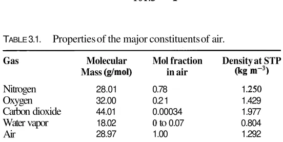
(K) for thermodynamic temperature, and the mole (mol) for the amount of substance. Units derived from these, which we use in this book are given in Table 1.1. Additional derived units can be found in Page and Vigoureux (1974).

TABLE 1.1. Examples of derived SI units and their symbols.

Quantity Name Symbol SI base units Derived Units

area volume velocity density force pressure-forcelarea energy chemical potential power concentration mol flux density heat flux density specific heat - - - - Newton Pascal joule - watt - - - - m2 m3 m s-I kg m-3 m kg s-2 kg m-I s-2 m2 _{kg s2} m2 _{s - ~} m2 _{kg s-3} mol mol m-2 s-I kg

s3

m2 s-2 K-I

-

- - -

-

N m-2 N m J kg-' J s-I

-

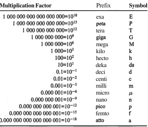
- W m-2 J kg-' K-'

To make the numbers used with these units convenient, prefixes are attached indicating decimal multiples of the units. Accepted prefixes, symbols, and multiples are shown in Table 1.2. The use of prefix steps smaller than lo3 is discouraged. We will make an exception in the use of the cm, since mm is too small to conveniently describe the sizes of things like leaves, and m is too large. Prefixes can be used with base units or derived units, but may not be used on units in the denominator of a derived unit (e.g., g/m3 _{or mg/m}3 _{but not mg/cm}3_{). The one exception to}

this rule that we make is the use of kg, which may occur in the denominator because it is the fundamental mass unit. Note in Table 1.2 that powers of ten are often used to write very large or very small numbers. For example, the number 0.0074 can be written as 7.4 x or 86400 can be written as 8.64 x lo4.

Most of the numbers we use have associated units. Before doing any computations with these numbers, it is important to convert the units to base SI units, and to convert the numbers using the appropriate multiplier from Table 1.2. It is also extremely important to write the units with the associated numbers. The units can be manipulated just as the numbers are, using the rules of multiplication and division. The quantities, as well as the units, on two sides of an equation must balance. One of the most useful checks on the accuracy of an equation in physics or engineering is the check to see that units balance. A couple of examples may help to make this clear.

Example 1.1. The energy content of a popular breakfast cereal is 3.9

Units

TABLE 1.2. Accepted SI prefixed and symbols for multiples and submultiples of units.

Multiplication Factor Prefix Symbol

exa

Pets

tera gigs mega kilo hecto deka deci centi milli micro nano pic0 femto atto

Solution. Table A.4 gives the conversion, 1 J = 0.2388 cal so

3.9kcal 103cal 103g

X - X - x 1 J = 16.3 x lo6

-

J

g kcal kg 0.2388 cal kg

= 16.3 MJ/kg.

Example 1.2. Chapter 2 gives a formula for computing the damping depth of temperature fluctuations

in

soil as D =

L-

k , where K is the

thermal diffusivity of the soil and

w

is the angular frequency of tem- perature fluctuations at the surface. Figure 8.4 shows that a typical dif- fusivity for soil is around 0.4mm2_{/s. Find the diurnal damping depth.}

Solution. The angular frequency is 2n/P, where P is the period of temperature fluctuations. For diurnal variations, the period is one day (see Chs. 2 & 8 for more details) so w = 2 n l l day. Converting w and K to SI base units gives:

2n 1 day 1 hr 1 min

w=- x

-

x

-

X - = 7.3 x 1 0 - ~ s-'

Example 1.3. Units for water potential are Jlkg (see Ch. 4). The gravita- tional component of water potential is calculated from llrg = - g z where g is the gravitational constant (9.8 and z is height (m) above a reference plane. Reconcile the units on the two sides of the equation.

Solution. Note from Table 1.1 that base units for the joule are kg m2 _s-2

so

The units for the product, gz are therefore the same as the units for @.

Confusion with units is minimized if the numbers which appear within mathematical operators ( J , exp,

In,

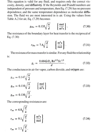
sin, cos, tan, etc.) are dimensionless. In most cases we eliminate units within operators, but with some empirical equations it is most convenient to retain units within the operator. In these cases, particular care must be given to specifying the units of the equation parameters and the result. For example, in Ch. 7 we compute the thermal boundary layer resistance of a flat surface from

where d is the length of the surface in m, u is the wind speed across the surface in d s , and rHa is the boundary layer resistance in m2 slmol. The constant 7.4 is the numerical result of evaluating numerous coefficients that can reasonably be represented by constant values. The constant has units of m2 _{s1/2/mol, but this is not readily apparent from the equation. If}

Problems 13

References

Page, C.H. and P. Vigoureux (1974) The International System of Units, Nat. Bur. Stand. Spec. Publ. 330 U.S. Govt. Printing Office, Washington, D.C.

Seeger, R.J. (1973) Benjamin Franklin, New World Physicist, New York: Pergamon Press.

Problems

1.1. Explain why a concrete floor feels colder to you than a carpeted floor, even though both are at the same temperature. Would a snake or cockroach (both poikilothem) arrive at the same conclusion you do about which floor feels colder?

1.2. In what ways (there are four) is energy transferred between living organisms and their surroundings? Give a description of the physical process responsible for eack and an example of each.

1.3. Convert the following to SI base units: 300 km, 5 hours, 0.4 rnm2/s,

25 kPa, 30 crnls, and 2 mmlmin.

1.4. In the previous edition ofthis book, and in much ofthe older literature, boundary layer resistances were expressed in units of slm. The units we will use are m2 _{slmol. To convert the old units to the new ones,}

divide them by the molar density of air (41.65 mol m-3 at 20' C and

101 Ha). If boundary layer resistance is reported to be 250 slrn, what is it in m2 _{slmol? What is the value of the constant in Eq. (1.3) if Ae}

Temperature

2

Rates of biochemical reactions within an organism are strongly depen- dent on its temperature. The rates of reactions may be doubled or tripled for each 10" C increase in temperature. Temperatures above or below critical values may result in denaturation of enzymes and death of the organism.

A living organism is seldom at thermal equilibrium with its microen- vironment, so the environmental temperature is only one of the factors determining organism temperature. Other influences are fluxes of radiant and latent heat to and from the organism, heat storage, and resistance to sensible heat transfer between the organism and its surroundings. Even though environmental temperature is not the only factor determining or- ganism temperature, it is nevertheless one of the most important. In this chapter we describe environmental temperature variation in the biosphere and discuss reasons for its observed characteristics. We also discuss methods for extrapolating and interpolating measured temperatures.

2.1

Typical Behavior of Atmospheric and Soil

Temperature

If daily maximum and minimum temperatures were measured at various heights above and below the ground and then temperature were plotted on the horizontal axis with height on the vertical axis, graphs similar to Fig. 2.1 would be obtained. Radiant energy input and loss is at the soil or vegetation surface. As the surface gets warmer, heat is transferred away from the surface by convection to the air layers above and by conduction to the soil beneath the surface. Note that the temperature extremes occur at the surface, where temperatures may be 5 to 10" C different from tem- peratures at 1.5 m, the height of a standard meteorological observation.

This emphasizes again that the microenvironment may differ substantially from the macroenvironment.

Temperature ( C )

FIGURE 2.1. Hypothetical profiles of maximum and minimum temperature above and below soil surface on a clear, calm day.

The fact that the temperature maximum occurs after the time of max- imum solar energy input is sigtllficant. This type of lag is typical of any system with storage and resistance to flow. Temperatures measured close to the exchange surface have less time lag and a larger amplitude than those farther from the surface. The principles involved can be illustrated by considering heat losses to a cold tile floor when you place your bare foot on it. The floor feels coldest (maximum heat flux to the floor) when your foot just comes in contact with it, but the floor reaches maximum temperature at a later time when heat flux is much lower.

The amplitude of the diurnal temperature wave becomes smaller with increasing distance from the exchange surface. For the soil, this is because heat is stored in each succeeding layer so less heat is passed on to the next layer. At depths greater than 50 cm or so, the diurnal temperature fluctuation in the soil is hardly measurable (Fig. 2.1).

Typical Behavior of Atmospheric and Soil Temperature 17

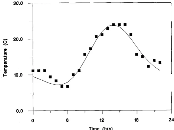
Time (hrs)

FIGURE 2.2. Hourly air temperature (points) on a clear fall day at Hanford, WA. The curve is used to interpolate daily maximum and minimum temperatures to obtain hourly estimates.

motion, or transport of parcels of hot or cold air over relatively long verti- cal distances, rather than by molecular motion. Within the first few meters of the atmosphere of the earth, the vertical distance over which eddies can transport heat is directly proportional to their height above the soil surface. The larger the transport distance, the more effective eddies are

in transporting heat, so the air becomes increasingly well mixed as one moves away from the surface of the earth. This mixing evens out the tem- perature differences between layers. This is the reason for the shape of the air temperature profiles in Fig. 2.1. They are steep close to the surface because heat is transported only short distances by the small eddies. Far- ther from the surface the eddies are larger, so the change of temperature with height (temperature gradient) becomes much smaller.

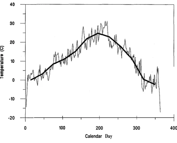
In addition to the diurnal temperature cycle shown in Fig. 2.2, there also exists an annual cycle with a characteristic shape. The annual cycle of mean temperature shown in Fig. 2.3 is typical of high latitudes which have a distinct seasonal pattern fiom variation in solar radiation over the year. Note that the difference between maximum and minimum in Fig. 2.3

is similar to the difference between maximum and minimum of the diurnal cycle in Fig. 2.2. Also note that the time of maximum temperature (around day 200) significantly lags the time of maximum solar input (June 2 1 ; day

-20

+

I I I I I I I

0 100 200 300 400

Calendar Day

FIGURE 2.3. Daily average temperature variation at Hanford, WA for 1978. The heavy line shows the monthly mean temperatures.

2.2

Random Temperature Variation

In addition to the more or less predictable diurnal and annual temperature variations shown in Figs. 2.2 and 2.3, and the strong, predictable spatial variation in the vertical seen in Fig. 2.1, there are random variations, the details of which cannot be predicted. We can describe them using statis- tical measures (mean, variance, correlation etc.), but can not interpolate or extrapolate as we can with the annual, diurnal, and vertical variations. Figure 2.3 shows an example of these random variations. The long-term monthly mean temperature shows a consistent pattern, but the daily av- erage temperature varies around this monthly mean in an unpredictable way. Figure 2.4 shows air temperature variation over an even shorter time. It covers a period of about a minute. Temperature was measured with a 25 p m diameter thermocouple thermometer.

The physical phenomena associated with the random variations seen in Figs. 2.3 and 2.4 make interesting subjects for study. For example, the daily variations seen in Fig. 2.3 are closely linked to weather patterns, cloud cover, and input of solar energy. The fluctuations in Fig. 2.4 are par- ticularly interesting because they reflect the mechanism for heat transport in the lower atmosphere, and are responsible for some interesting optical phenomena in the atmosphere.

Random Temperature Variation 19

0 10 20 30 40 50 60 70

Time (s)

FIGURE 2.4. Air temperature 2 m above a desert surface at White Sands Missile Range, NM. Measurements were made near midday using a 25 pm diameter thermocouple.

differ substantially from the mean air temperature that one might measure with a large thermometer. The relatively smooth baseline in Fig. 2.4, with jagged interruptions, indicates a suspension of hot ascending parcels in a matrix of cooler, descending air. Well mixed air is subsiding, being heated at the soil surface, and breaking away from the surface as convective bubbles when local heating is sufficient.

Warm air is less dense than cold air, and therefore has a lower index of refraction. As light shines though the atmosphere, the hot and cold parcels of air act as natural lenses, causing the light to constructively and destructively interfere, giving rise to a diffraction pattern. Twinkling of stars and the scintillation of terrestrial light sources at night are the result of this phenomenon. The diffraction pattern is swept along with the wind, so you can look at the lights of a city on a clear night from some distance and estimate the wind speed and direction from the

drift

of the scintillation pattern.

look like water. This is the result of the systematic vertical variation in temperature above the heated surface, rather than the result of the random variations that we were just discussing.

Air temperatures are often specified with a precision of 0.5" to 0. lo C. From Fig. 2.4 it should be clear that many instantaneous temperature measurements would need to be averaged, over a relatively long time period, to make this level of precision meaningful. Averages of many readings, taken over 15 to 30 minutes, are generally used. Figures 2.1 and 2.2 show the behavior of such long-term temperature averages. Large thermometers can provide some of this averaging due to the thermal mass of the sensing element.

Random temperature variations are, of course, not limited to the time scales just mentioned. Apparently random variations in temperature can be shown from the geologic record, and were responsible, for example, for the ice ages. There is considerable concern, at present, about global warming and climate change, and debate about whether or not the climate has changed. Clearly, there is, always has been, and always will be climate change. The more important question for us is whether human activity has or will measurably alter the random variation of temperature that has existed for as long as the earth has been here.

2.3

Modeling Vertical Variation in Air

Temperature

The theory of turbulent transport, which we study in Ch. 7, specifies the shape of the temperature profile over a uniform surface with steady-state conditions. The temperature profile equation is:

where T ( z ) is the mean air temperature at height

z,

To is the apparent aerodynamic surface temperature,

zH

is a roughness parameter for heat transfer, H is the sensible heat flux from the surface to the air,

jk,

is the volumetric specific heat of air (1200 J m-3 C-' at 20" C and sea level), 0.4 is von Karman's constant, and u* is the friction velocity (related to the friction or drag of the stationary surface on the moving air). The reference level from which

z

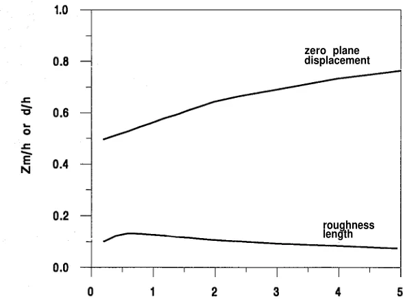
is measured is always somewhat arbitrary, and the correction factor d , called the zero-plane displacement, is used to adjust for this. For a flat, smooth surface, d = 0. For a uniformly vegetated surface, Z H 1:0.02h, and d 1:0.6h, where h is canopy height.

We derive Eq. (2.1) in Ch. 7, but use it here to interpret the shape of the temperature profile and extrapolate temperatures measured at one height to other heights. The following points can be made.

Modeling Vertical Variation in Air Temperature 21

2. Temperature increases with height when H is negative (heat flux to- ward the surface) and decreases with height when H is positive. During the day, sensible heat flux is generally away from the surface so T decreases with height.

3. The temperature gradient at a particular height increases in magnitude as the magnitude of H increases, and decreases as wind or turbulence increases.

Example 2.1. The following temperatures were measured above a 10 cm high alfalfa crop on a clear day. Find the aerodynamic surface temperature,

To

-

Height (m) 0.2 0.4 0.8 1.6 Temperature (C) 26 24 23 21

Solution. It can be seen from Eq. (2.1) that T (z) = To when the In term is zero, which happens when z = d

+

ZH since ~ ( Z H / Z H ) = ln(1) = 0.

If h[(z - d)/zH] is plotted versus T (normally the independent variable is plotted on the abscissa or horizontal axis, but when the independent variable is height, it is plotted on the ordinate or vertical axis) and ex- trapolate to zero, the intercept will be To. For a 10 cm (0.1 m) high canopy, zH = 0.002 m, and d = 0.06 m. The following can therefore be computed:

-

Height (m) 0.2 0.4 0.8 1.6 Temp. (C) 26 24 23 21 (Z - ~ ) / z H 70 170 370 770 I~[(z

-

~ ) / z H ] 4.25 5.14 5.91 6.65.

The Figure for Example 2.1 on the following page is plotted using this data, and also shows a straight line fitted by linear least squares through the data points that is extrapolated to zero on the log-height scale. The intercept is at 34.6" C, which is the aerodynamic surface temperature.

20 25 30 35

Temperature (C)

Solution. This problem could be solved by plotting, as we did inExample 1, or it could be done algebraically. Here we use algebra. The constants, H/(0.4pcPu*) in Eq. (2.1) are the same for all heights. For convenience, we represent them by the symbol A . Equation (2.1) can then be written for each height as

Subtracting the second equation from the first, and solving for A gives

A = -2.25" C. Substituting this back into either equation gives To =

-8.6" C. Knowing these, now solve for T(h) where h = 0.5 m:

So the top of the canopy is below the freezing temperature.

Soil Temperature Changes with Depth and Time

2.4

Modeling Temporal Variation in Air

Temperature

Historical weather data typically consist of measurements of daily max-

imum and minimum temperature measured at a height of approximately 1.5 m. There are a number of applications which require estimates of hourly temperature throughout a day. Of course, there is no way of know- ing what the hourly temperatures were, but a best guess can be made by assuming that minimum temperatures normally occur just before sunrise and maximum temperatures normally occur about two hours after solar noon. The smooth curve in Fig. 2.2 shows this pattern. The smooth curve was derived by fitting two terms of a Fourier series to the average of many days of hourly temperature data which had been normalized so that the minimum was 0 and the maximum was 1. The dimensionless diurnal temperature function which we obtained in this way is:

where w = n/12, and t is the time of day in hours (t = 12 at solar noon). Using this function, the temperature for any time of the day is given by

T(t) = Tx,i-~r(t>

+

Tn,i[l

-

r(t>I O < t 1 5

T(t) = Tx,ir(t)

+

Tn,i[l

-

r(t>I 5 < t 5 14 (2.3) T(t) = Tx,ilr(t)

+

Tn,i+l[l - r(t)I 14 < t < 24.

Here, Tx is the daily maximum temperature and Tn is the minimum tem- perature. The subscript i represents the present day; i - 1 is the previous day, and i

+

1 is the next day. The curve in Fig. 2.2 was drawn using Eqs. (2.2) and (2.3). Note that t is solar time. The local clock time usually differs from solar time, so adjustments must be made. These are discussed in detail in a later chapter.

Example 2.3. Estimate the temperature at 10 AM on a day when the

minimum was 5" C and the maximum was 23" C.

Solution. At t = 10 hrs, (note that angles are in radians)

+

0.11 sin

(

2 x 3.14 x 10 12

Since 10 is between 5 and 14, the middle form of Eq. (2.3) is used, so

2.5

Soil Temperature Changes with Depth and

Time

variation with depth in soil. The features to note are that the temperature extremes occur at the surface where radiant energy exchange occurs, and that the diurnal variation decreases rapidly with depth in the soil. Figure 2.5 also shows these relationships and gives additional insight into soil temperature variations. Here, temperatures measured at three depths are shown.

Note that the diurnal variation is approximately sinusoidal, that the am-

plitude decreases rapidly with depth in the soil, and that the time of maxi- mum andminimum shifts with depth. At the surface, the time ofmaximum temperature is around 14:OO hours, as it is in the air. At deeper depths the times of the maxima and minima lag solar noon even farther, and at 30 to 40 cm, the maximum is about 12 hours after the maximum at the surface. We derive equations for heat flow and soil temperature later when we discuss conductive heat transfer. For the moment, we just give the equation which models temperatures in the soil when the temperature at the surface is known. This model assumes uniform soil properties throughout the soil profile and a sinusoidally varying surface temperature. Given these assumptions, the following equation gives the temperature as a function of depth and time:

1

0 6 12 18 24 30 36 42 48

Time (hrs)

Soil Temperature Changes with Depth and Time 25

where Tave is the mean daily soil surface temperature, o is n/12, as in Eq. (2.2), A(0) is the amplitude of the temperature fluctuations at the surface (half of the peak-to-peak variation) and D is called the damping depth. The "-8" in the sine function is a phase adjustment to the time variable so that when time t = 8, the sine of the quantity in brackets is zero at the surface (z = 0). We discuss computation of diurnal damping depth in Ch. 8. It has a value around 0.1 m for moist, mineral soils, and 0.03 to 0.06 m for dry mineral soils and organic soils.

In many cases we are not interested in the time dependence of the soil temperature, but would just like to know the range of temperatures at a particular depth. It is known that the range of the sine function is

-

1 to 1 so Eq. (2.4) gives the range of soil temperature variation as

where the

+

gives the maximum temperatures and the

-

the minimum.

Example 2.4. At what depth is the soil temperature within

f

0.5" C of the mean daily surface temperature if the temperature variation at the surface (amplitude) is

f

15" C?

Solution. The amplitude of the desired temperature variation is 0.5" C. Rearranging Eq. (2.5) and taking the logarithm of both sides gives

If D = 12cm, then the depth for diurnal variations less than k0.5"C would be 3.4 x 12 cm = 41 cm. Therefore a depth of at least 40 cm needs to be dug to obtain a soil temperature measurement that is not influ- enced by the time of day the temperature is measured.

The annual soil temperature pattern is similar to the diurnal one, but with a much lower frequency and a much larger damping depth. Equa- tions (2.4) and (2.5) are used to describe the annual variation, but D is around 2 m, and o is 2x1365 days.

While Eqs. (2.4) and (2.