Can Economic Growth be Inclusive and Immiserising? The Kuznets Hypothesis and ‘Premature Deindustrialisation’
Arief Anshory Yusuf *, Andy Sumner** & Ekki Syamsulhakim* * Padjadjaran University, Indonesia and ** King’s College London, UK
Draft
–
please do not cite or circulate
1. Introduction
In this paper, we use district level data from Indonesia to consider how economic growth has impacted poverty and inequality during a period of ‘premature deindustrialisation’. To put our
findings in context and to build new theory, we revisit the ‘Kuznets hypothesis’ and review writing in the tradition of Kuznets. We then hypothesise a new relevance of Kuznets to developing countries experiencing ‘premature deindustrialisation’. The paper is structured as
follows. Section 2 discusses the literature on poverty, inequality and growth. Section 3 considers the case of Indonesia. Section 4 revisits Kuznets. Section 5 concludes.
2. Poverty, inequality and growth
Numerous scholars have, without doubt, given considerable attention to the poverty, inequality and growth relationship in developing countries. Historically, the interest in the broad area– defined as who benefits from growth and how much – grew from debates in the early 1970s that were critical of the distribution of the benefits of growth at that time (e.g., Adelman and Morris, 1973; Chenery et al., 1974). Such issues received considerable attention in the late 1990s through to the mid-2000s under different umbrella terms. For example, ‘growth with equity’ which drew on controversial debates on East Asian development (see, for example, Fei
et al., 1979; Jomo, 2006; World Bank, 1993). At that time, growth with equity was replaced by the label of ‘pro-poor’ growth (see, for example, Besley and Cord, 2006; Grimm et al., 2007;
became the umbrella term for considering who benefits from growth.1 .
The body of literature provides the empirical basis for the accepted notion that economic growth is inclusive in a general sense: on average, the poverty headcount falls and the incomes of the poorest rise in line with average income growth (see Dollar and Kraay, 2002; Kraay, 2006; Dollar et al., 2013). However, two recent contributions have reopened this debate. First, Shaffer (2015) notes that in 10-15 per cent of episodes, poverty actually rises with growth and he connects this with historical debates on ‘immiserising growth’. Second,
Sen (2013) concurs with this finding in that there are a surprising number of growth episodes that are not inclusive (i.e., episodes are without falling poverty and/or with rising inequality). Sen separates types of growth episodes between ‘growth acceleration’ and ‘growth maintenance’ and finds that the former is much less likely to benefit the poor than the latter.
Sen argues that this is because the institutional factors that lead to growth accelerations are different from those that lead to growth maintenance.2 This points towards a well noted argument that the average inclusivity of growth can be misleading as it is subject to enormous variation across countries and highly sensitive to where the poverty line is set (see also the
1The various labels differ from each other in nuances. For example, ‘growth with equity’ was typically defined as growth during which inequality does not rise or may even fall (and it is a term associated with World Bank, 1993). In contrast, absolute pro-poor growth was defined as growth with a falling poverty headcount (or rising incomes of the poor measured by a poverty or fractile line); relative pro-poor growth, on the other hand, is considered to occur if that fall in the poverty headcount is accompanied by falling inequality of outcome (see
discussions in Kakwani and Pernia, 2000; Ravallion, 2004). ‘Inclusive growth’ was defined as poverty reduction
both in monetary and non-monetary terms. This implied the participation of the poor – or a broader group beyond just the poor – in growth processes via employment and the expansion of capabilities (in terms of public goods access) which reduces poverty and potentially reduces the inequality of opportunity as well as the inequality of
outcomes. The term ‘shared prosperity’, is one more label sitting under the umbrella of ‘inclusive growth’. It is a
term associated with the World Bank (e.g., World Bank, 2016), and is defined specifically as the income growth of the poorest 40 per cent of population. The relationship between multidimensional poverty and growth is more complex than the mathematical identity of monetary poverty. Santos et al. (2016) find the relationship between multidimensional poverty and growth to be much weaker than monetary poverty and growth. Rising incomes among the monetary or multidimensional poor can lead to improved nutrition intake and outcomes or improved access to education and health and outcomes but public spending may be important in terms of the provision of free or subsidised public education and health. Social policy such as redistributive transfers can further support the reduction of both monetary and multidimensional poverty (for a discussion of countries with multidimensional poverty data over time, see Alkire et al., 2011).
discussions of Edward and Sumner, 2015). Much of the debate turns on whether inequality is high or rising, as high and rising inequality can hamper not only poverty reduction but also future growth prospects, which can impact future poverty reduction.3
What variables are thought in the literature to explain such cross-country variations?
The role of initial inequality is most often cited in determining the responsiveness of poverty
to growth. Specifically, that the extent of poverty reduction depends on prevailing inequality
levels and that a higher level of initial inequality leads to less poverty reduction at any given
level of growth which is a mathematical identity (see Adams, 2003; Deininger and Squire,
1998; Fosu, 2011; Hanmer and Naschold, 2001; Kalwij and Verschoor, 2007; Misselhorn and
Klasen, 2006; Ravallion, 1995, 1997, 2001, 2004, 2005a, 2005b; Son and Kakwani, 2003;
Stewart, 2000). A recent observation is – perhaps Kuznets revenge – that rapid growth with
structural change is associated with rising inequality in many developing countries such as
Indonesia (see Sumner, 2016). Although this is not a very large set of countries experiencing
growth with structural change data on decile shares to the richest decile corroborate rising
inequality with fast growth. That said of course governments are not impotent and the range of
policies to manage inequality is well known (see UNDP, 2010).
3. The case of Indonesia
3a. Poverty, inequality and growth
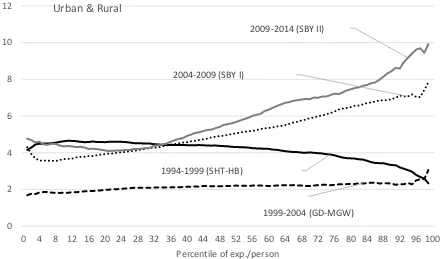
Growth incidence curves (GICs) provide one way to visualise the poverty, inequality and growth relatonship beyond simply presenting elasticities. Figure 1 shows the growth incidence curves for different administrations in Indonesia from 1994-2014. Figure 1 shows that, with the exception of the period of 1994-1999, the Soeharto-Habibie (ST-HB) era, the Indonesian growth incidence curve for all administrations before Jokowi has always been upward-sloping. Comparing the growth-incidence-curves (GIC) for four different adminstrations, one general observation is that the period of Yudhoyono (SBY) presidency (2004-2014) is the period of the most rapidly rising prosperity. However, as can be seen from the slope of the GICs, these periods are also the most unequalising. The later SBY term (2009-2014) is notable in that during this period the expenditure per capita of the top 5% grew annually at 10% (see the second panel of Figure 1). The period is the period where Indonesia experienced the greatest increase in consumption inequality (see below).
boom. Of course this is insufficient to establish causation though it does provide a clear correlation between rising commodity prices and inequality in Indonesia.
Looking carefully the GIC under the second SBY term for the poorest 30% of the population, we can make two observations: First, up-to approximate the 30th percentile the slope is downward sloping. This means that the expenditure of the very poor increased more than the less-poor. Second, the rural poor experienced higher expenditure growth than the urban poor.4 One of the important milestones in the development of social protection programs in Indonesia during the second SBY term was the introduction of a unified database for beneficiaries to support the implementation of targeted social assistance. TNP2K (Tim Nasional Percepatan Penangulangan Kemiskinan), a new body replacing the earlier coordinating agency, TKPK (which did not have authority, capacity and resources to the same extent) was behind the effort of the database unification. TNP2K was also given responsibility to oversee the coordination of household-based social assistance programs, community empowerment programs, and programs to expand economic opportunities for low-income households (Sumarto and Suryadarma, 2011).
Figure 1. Growth incidence curves under various administrations (Percentage change in real expenditure per person by percentile of expenditure per person), 1994-2014
Source: Authors’ calculation based on SUSENAS
The major social protection programs include the rice for the poor (Raskin), conditional cash transfers (CCT), and national community health insurance (Jamkesnas). The negative slope of the GIC at the bottom part of the population could be explicable by the following (non mutually exclusive) factors: (i) social assistance or social protection received by the poor generated larger proportionate increases in their income and eventually spending, generating a downward sloping GIC; (ii) Some social protection programs introduced during this period targeted the very poorest such as the conditional cash transfer program (PKH). As above, further research is needed to establish causality between the social assistance programs and the shape of the GIC during the same period.
A downward sloping growth-incidence-curve also occurred during the Soeharto-Habibie period (1994-1999). During this period everyone benefited from economic growth as
1994-1999 (SHT-HB)
1999-2004 (GD-MGW) 2004-2009 (SBY I)
2009-2014 (SBY II)
0 2 4 6 8 10 12
0 4 8 12 16 20 24 28 32 36 40 44 48 52 56 60 64 68 72 76 80 84 88 92 96 100 Percentile of exp./person
but the richer less so (proportionally to their initial level) than the poor. This may relate to the Asian Financial Crisis of 1997/98. The deterioration of Indonesian currency, the collapse of the banking and financial sectors that happened during the crisis would have tended to hurt the rich more than the poor though all of society was hit by the crisis. The period of the recovery from the crisis (1999-2004) under the presidency of Abdurrahman Wahid (or Gus Dur) and later on Megawati was a period of the lowest growth in expenditure. The flatness of the GIC of this period indicates equal benefits of growth during that period.
Next, we link changes in poverty to growth elasticities. Table 1 thus seeks to compare administrations. The period of 1994-1999 (Soeharto-Habibie) was successful in reducing multidimensional poverty despite the crisis. As noted above the fact that the elasticity of multidimensional poverty to growth is high in the period interrupted by the economic crisis may suggest the lower correlation of multidimensional poverty to economic business cycles. We conclude that the SBY period was the least successful in term of generating poverty reduction for every 1% economic growth. This applies to both the poverty incidence by the national poverty line or multidimensional poverty incidence. In contrast, the Megawati and Gus-Dur period had made a 2% reduction in multidimensional poverty for every 1% economic growth.
Table 1. Growth, change in poverty incidence by national poverty line, 1994-2014
Growth
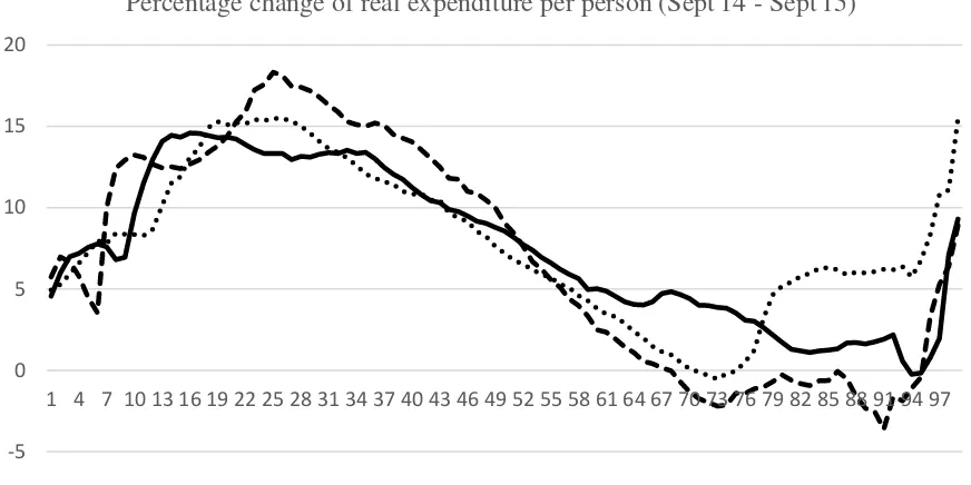
Figure 2. Growth incidence curve for Jokowi’s presidency, Sept. 2014 to Sept 2015 Source: Authors’ calculation
Source: Authors’ calculation based on SUSENAS
Jokowi’s administration could be judged against the baseline of his predecessors. We
concluded above that economic growth between 1994 and 2014 has been accompanied by an impressive decline in multidimensional poverty and moderate progress in reducing monetary poverty incidence. Inequality, however, has risen to an unprecedented magnitude, particularly during the period of SBY (2004-2014). Moreover, the rate of the reduction in both monetary poverty and multidimensional poverty has been slowing.
Figure 2 shows the growth incidence curve for the first year of the Jokowi presidency, from September 2014 to September 2015. We should note that the first 6 months of Jokowi’s term, food inflation was very high. The price of rice reached its peak in March, when BPS conducted the Susenas survey. The price of rice increased by around 16% over the six months (Yusuf and Sumner, 2015). From Table 2, we see that from September 2014 to March 2015, poverty incidence by the national poverty line increase by 0.26% (and increased 0.13% in urban and 0.45% in rural areas). This sounds like a small increase but represents a million extra poor
-5 0 5 10 15 20
1 4 7 10 13 16 19 22 25 28 31 34 37 40 43 46 49 52 55 58 61 64 67 70 73 76 79 82 85 88 91 94 97 Percentage change of real expenditure per person (Sept'14 - Sept'15)
people. The increase in poverty is most likely due to: (i) the slowing down of economic growth and hence weaker employment growth; (ii) an increase in the price of rice5; and (iii) The delayed disbursement of cash compensation intended to protect the poor from the impact of the fuel price increase in November 20156 (See Yusuf and Sumner, 2015).
The growth incidence curve (for the first year of the Jokowi administration) shows that the upper middle income group, particularly those close to the top 10% saw their expenditure fall, particularly in urban area. Some caution is required though in interpretation of this. This dynamic is most likely cyclical and related to the nature of the slowing down of the economy which is characterized by resource and capital-intensive (and most likely skill-intensive) sector being the hardest hit. This is supported by the figure which shows that urban upper middle class suffered more than rural upper middle class.
Table 2. Changes in poverty incidence and inequality under Jokowi’s administration
Poverty incidence Gini coefficient Palma Ratio
Urban Rural All Urban Rural All Urban Rural All
5 Our simulation, using Susenas data, suggests that for every 1% increase in the price of rice, the national poverty headcount will increase by more than 1% (with other factors held constant).
The nature of the distribution of economic growth (as shown by the GIC curves) implies a slight decline in inequality nationally and in urban areas. However, the magnitude of the change is not that significant and discussion of a change in inequality over such as short period of time is questionable.
The official BPS poverty estimates based on that Susenas suggest that the poverty incidence still increased over the one year period. However, there is small improvement on the March 2015 position, but the poverty incidence in September 2015 is still higher compared to the previous one year. It suggest that during the first year of Jokowi’s administration, the
poverty incidence rose, nationally by 0.17% (0.06% in urban area and 0.33% in rural areas). As a result of this, and in contrast to the previous 4 administrations, Jokowi’s first year has a
positive growth elasticity of poverty. This specifically meaning that for every one per cent of economic growth generated, poverty increase by 0.04% percentage point.
In sum, although the aspirations and the budgetary reform undertaken, the first year of Jokowi’s presidency has been less successful in term of the inclusiveness of growth compared
to previous administrations. That said, the outlook for the remaining period of the current administration is likely to be more position given changes in social spending. The inclusivity of growth will depend on whether the large increase in physical infrastructure investment generates inequality-reducing economic growth via its employment generation impacts; whether the government’s budget, particularly in targeted social spending, in education and
3b. Urban and rural poverty, inequality and growth in Indonesia: An econometric analysis
The figure below plots the annualised change in the poverty headcounts (by the national poverty line which is very close to the global poverty line of $1.90) of around 300 districts in Indonesia for the period of 2002-2012 against the economic growth during the same period. It suggests that most districts that have positive economic growth per capita experienced a decline in poverty incidence. However, we can observe from the plot that districts that are classified as urban areas are clustered around a smaller change in poverty incidence even when they have high economic growth. There are quite a number of cities with rises in poverty incidence despite positive or even substantially above-national-average economic growth during the period. One plausible explanation for this is that the rural poor migrate and become the urban poor though other factors are likely to also play a role.
Econometric analysis
We model changes in poverty incidence as a function of economic growth, initial poverty incidence, initial inequality and cities dummies, and model change in the Gini coefficient as a function of overall and sectoral growth, initial Gini coefficient and cities dummies. We use rainfall data for each district as instrumental variable for economic growth to estimate the models using an instrumental variable (IV) regression. This takes into account the problem of endogeneity (which may bias the estimate of the effect of growth on the dependent variables – i.e., the changes in poverty and inequality – and may thus invalidate causal claims).
Data and Methodology
We use the INDODAPOER (Indonesian Database for Policy and Economic Research) data to examine whether growth has been immiserising in Indonesia. This data is available for public
-2
-1
0
1
-20 -10 0 10 20
Annual change in total GDP per person
use and downloadable from the World Bank’s micro-data website. INDODAPOER covers
information related to the economy, infrastructure, education, health, poverty, labor and social protection, and financial sectors at the district- and province-level from 1976 to 2014. There are 219 variables from 546 districts covered in the data to date. For our analysis, we choose the period of 2002 – 2012, which as discussed earlier, an era of democratization and decentralization in Indonesia. The included districts in our analysis is 295, consisting of 64 urban and 231 rural areas. We ended up with much less districts partly due to the grouping of expanded districts.
As mentioned above, we basically develop two econometric models. The first model is intended to investigate factors affecting changes in poverty incidence, whereas the second is formed to examine factors affecting changes in inequality. Included as the independent variables in the first model are economic growth, initial poverty incidence, and some other covariates such as city dummies, literacy rate for population above 15 years old, different level of education participation (net enrolment ratio of school aged children in primary, junior secondary and senior secondary school in each districts), and infrastructure conditions (household access to electricity, safe water, and sanitation). Similar to the first model, the covariates included in the second model are sectoral economic growth, initial gini coefficient, and also other variables included in the first model.
𝑐ℎ𝑔𝑝𝑜𝑣𝑖 = 𝛽0+ 𝛽1𝑔𝑟𝑜𝑤𝑡ℎ𝑖+ 𝛽2𝑖𝑛𝑖𝑡𝑝𝑜𝑣𝑖+ ∑ 𝛽𝑗𝑥𝑗𝑖+ 𝑢𝑖, 𝑗 = 3, … , 𝐽 (1)
and
𝑐ℎ𝑔𝑔𝑖𝑛𝑖𝑠= 𝛽0+ 𝛽1𝑔𝑟𝑜𝑤𝑡ℎ𝑠+ 𝛽2𝑖𝑛𝑖𝑡𝑔𝑖𝑛𝑖𝑖+ ∑ 𝛽𝑗𝑥𝑗𝑠+ 𝑢𝑠, 𝑗 = 3, … , 𝐽 (2)
As growth may potentially be endogenous, we use rainfall data for each district to act as the instrument for growth, and employ an Instrumental Variable (IV) regression to estimate the coefficients of the models. Rainfall is chosen as the instrument because it is correlated with growth and not correlated with the unobserved heterogeneity that may affect changes in poverty incidents or change in inequality (Bhattacharyya and Resosudarmo, 2013).
There are different ways of how rainfall should enter the first stage regression. Miguel, et.al (2004, page 737), for example, use the growth of rainfall as the instruments for economic growth. Meanwhile, Sarsons (2015) uses the level-data of rainfall as instruments, arguing that the growth of rainfall may mistakenly identify rain shocks. In our case, we follow Bhattacharyya and Resosudarmo (2013) and Sarsons (2015) method in treating our rainfall variable.
Specifically, the reduced form for growth in equation (1) and (2) can be written as
𝑔𝑟𝑜𝑤𝑡ℎ𝑖= 𝜋0+ 𝜋1𝑟𝑎𝑖𝑛𝑓𝑎𝑙𝑙𝑖+ ∑ 𝜋𝑗𝑥𝑗𝑖+ 𝑣𝑖, 𝑗 = 2, … , 𝐽 (3)
where 𝑖 denotes districts, and
𝑔𝑟𝑜𝑤𝑡ℎ𝑠= 𝛾0+ 𝛾1𝑟𝑎𝑖𝑛𝑓𝑎𝑙𝑙𝑠+ ∑ 𝛾𝑗𝑥𝑗𝑠+ 𝜔𝑠, 𝑗 = 2, … , 𝐽 (4)
where 𝑠 denotes sectors.
In addition, we also have attempted to do several specifications in finding the best IV specification. First, we intentionally choose the rainfall data on one specific month in a year which yields the highest relevant statistical values as our instrument for growth. Second, we use all of the monthly rainfall data in a year as the exogenous instruments. Third, we use the annual average of the rainfall as the instruments.
the bottom of the tables). Those sectors may not be directly impacted by the changes in precipitation. The second approach statistically provides more consistent evidence that rainfall is partially correlated with growth, albeit showing a lower value of F-statistics than the first method. Finally, the third approach can be seen as the weakest instrument for growth, as it rarely provides a statistically significant first-stage regression statistics.
17
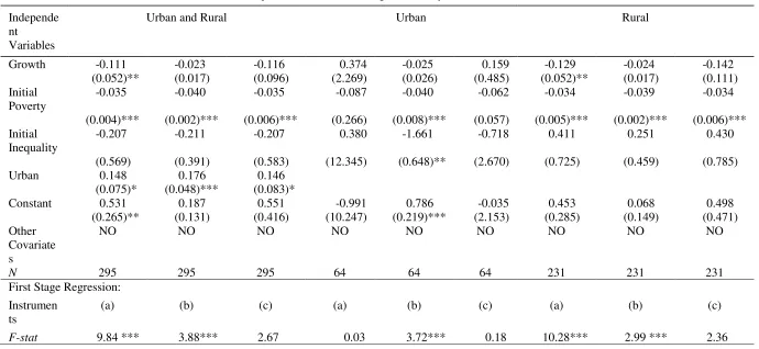
Table 37
Dependent Variable : Change in Poverty 2002 – 2012
Independe
7(a) intentionally choose the rainfall data on one specific month in a year which yields the highest relevant statistical values; (b) monthly rainfall data (linear combination
19
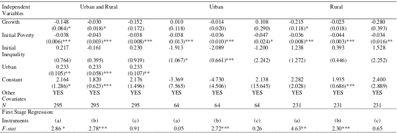
Table 4
Dependent Variable : Change in Poverty 2002 – 2012
Independent Variables
Urban and Rural Urban Rural
Growth -0.148 -0.030 -0.152 0.010 -0.014 0.108 -0.215 -0.025 -0.280
(0.084)* (0.018)* (0.172) (0.118) (0.020) (0.290) (0.118)* (0.018) (0.393)
Initial Poverty -0.038 -0.043 -0.038 -0.038 -0.036 -0.047 -0.036 -0.044 -0.034
(0.006)*** (0.003)*** (0.008)*** (0.013)*** (0.010)*** (0.024)* (0.008)*** (0.003)*** (0.016)**
Initial Inequality
0.217 -0.161 0.230 -1.913 -2.089 -1.200 1.238 0.393 1.528
(0.764) (0.395) (0.919) (1.067)* (0.661)*** (2.242) (1.272) (0.446) (2.252)
Urban 0.233 0.233 0.233
(0.105)** (0.058)*** (0.107)**
Constant 2.164 1.820 2.176 -3.369 -4.730 2.138 2.282 1.935 2.400
(1.286)* (0.623)*** (1.496) (7.565) (4.506) (15.645) (2.028) (0.686)*** (2.889)
Other Covariates
YES YES YES YES YES YES YES YES YES
N 295 295 295 64 64 64 231 231 231
First Stage Regression:
Instruments (a) (b) (c) (a) (b) (c) (a) (b) (c)
F-stat 2.86 * 2.78*** 0.91 0.05 2.72*** 0.26 4.63** 2.30*** 0.65
20
Table 5
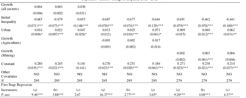
Dependent Variable : Change in Inequality 2002 – 2012
Growth
(all sectors) -0.004 0.003 0.030
(0.006) (0.002) (0.031)
Initial
Inequality -0.685 -0.679 -0.655 -0.687 -0.677 -0.644 -0.691 -0.662 -0.641
(0.071)*** (0.073)*** (0.148)*** (0.070)*** (0.074)*** (0.129)*** (0.079)*** (0.078)*** (0.100)***
Urban 0.016 0.022 0.047 0.013 0.025 0.071 0.009 0.040 0.062
(0.008)* (0.007)*** (0.028)* (0.012) (0.010)*** (0.041)* (0.015) (0.012)*** (0.031)**
Growth
(Agriculture) -0.003 0.002 0.017
(0.003) (0.002) (0.014)
Growth
(Mining) -0.002 0.003 0.006
(0.002) (0.001)*** (0.004)
Constant 0.280 0.245 0.101 0.270 0.251 0.186 0.271 0.238 0.214
(0.035)*** (0.021)*** (0.161) (0.023)*** (0.020)*** (0.063)*** (0.025)*** (0.021)*** (0.037)***
Other
Covariates NO NO NO NO NO NO NO NO NO
N 295 295 295 295 295 295 279 279 279
First Stage Regression:
Instruments (a) (b) (c) (a) (b) (c) (a) (b) (c)
F-stat 9.84*** 3.88*** 2.67 16.37*** 2.77*** 3.65* 9.20*** 4.08*** 4.37**
21
Table 6
Dependent Variable : Change in Inequality 2002 – 2012
Growth (manufacture)
-0.006 0.003 0.023
(0.011) (0.003) (0.024)
Initial Inequality -0.734 -0.656 -0.494 -0.708 -0.643 -0.599 -0.709 -0.596 -0.596
(0.133)*** (0.076)*** (0.324) (0.089)*** (0.079)*** (0.110)*** (0.083)*** (0.081)*** (0.085)***
Urban 0.007 0.026 0.066 0.012 0.031 0.043 0.019 0.024 0.024
(0.023) (0.009)*** (0.044) (0.013) (0.008)*** (0.014)*** (0.007)*** (0.007)*** (0.007)***
Growth (utility)
-0.003 0.005 0.010
(0.005) (0.002)** (0.006)*
Growth (Construction)
-0.002 0.005 0.005
(0.002) (0.001)*** (0.002)**
Constant 0.303 0.238 0.103 0.288 0.218 0.172 0.277 0.205 0.205
(0.082)*** (0.024)*** (0.182) (0.048)*** (0.026)*** (0.052)*** (0.032)*** (0.024)*** (0.030)***
Other Covariates NO NO NO NO NO NO NO NO NO
N 295 295 295 295 295 295 295 295 295
First Stage Regression:
Instruments (a) (b) (c) (a) (b) (c) (a) (b) (c)
F-stat 1.05 2.15** 1.98 6.53** 2.03** 6.56** 13.63*** 3.47*** 12.81***
22
Table 7
23
Table 8
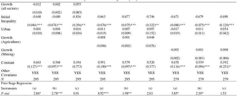
Dependent Variable : Change in Inequality 2002 – 2012
Growth (all sectors)
-0.012 0.002 0.055
(0.010) (0.002) (0.085)
Initial Inequality
-0.640 -0.680 -0.836 -0.663 -0.677 -0.746 -0.671 -0.679 -0.690
(0.084)*** (0.074)*** (0.356)** (0.076)*** (0.075)*** (0.322)** (0.088)*** (0.075)*** (0.120)***
Urban 0.001 0.004 0.016 -0.011 0.007 0.097 -0.017 0.011 0.054
(0.010) (0.008) (0.036) (0.015) (0.009) (0.152) (0.019) (0.011) (0.042)
Growth (Agriculture)
-0.008 0.001 0.048
(0.006) (0.002) (0.076)
Growth (Mining)
-0.003 0.001 0.008
(0.002) (0.001) (0.006)
Constant 0.663 0.568 0.194 0.591 0.579 0.520 0.670 0.559 0.392
(0.127)*** (0.097)*** (0.773) (0.100)*** (0.097)*** (0.377) (0.116)*** (0.096)*** (0.231)*
Other
Covariates YES YES YES YES YES YES YES YES YES
N 295 295 295 295 295 295 279 279 279
First Stage Regression:
Instruments (a) (b) (c) (a) (b) (c) (a) (b) (c)
F-stat 2.86* 2.78*** 0.91 8.92*** 1.98** 2.03 3.85* 2.39* 1.53
24
Table 9
Dependent Variable : Change in Inequality 2002 – 2012
25
Table 10
26
Discussion
Table 3-10 report various regression results. Table 3 and 4 reports the estimation of the poverty model, while table 5-10 reports the estimation of the inequality model. For poverty model, the benchmark specification is that change in poverty is a function of growth, initial poverty incidence, initial inequality and areas (urban-rural). The first table report the benchmark model, the second table add other relevan correlates of poverty incidences to account for more control variable. What we will be discussed further here is the later tables which report the estimation results with all covariates. The benchmark is for comparison purpose only. As also mentioned previously, the table also report results with different variations of how we measure instrumental variables.
As can be seen from Table 2, the effect of growth on poverty reduction is rather mixed. As we include initial poverty incidence (which is actually strong and statistically significant), we are actually testing whether districts with similar initial level of poverty incidence will experience faster poverty reduction episodes when their economic growth is higher. The result suggest yes if we look at nationally as economic growth is negative and significant (despite only marginally at 10% level). However, when we divide sample into urban (cities) and rural (non-cities) districts, the economic growth is not significant for urban samples. It should be noted that we are refering to the regression results with the strongest instruments (with the highest F-statistics in the first stage regression). The national level regression also suggests that controlling for growth and initial poverty incidence, urban districts tend to have slower poverty reduction as the coefficient of the city dummies is strongly significant.
27
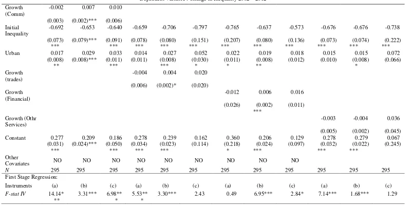
inequality level with is associated with faster absolute change in inequality and vice versa. In terms of the impact of growth, the regression results suggest that at aggregate level economic growth does not have any effect on inequality. That is said it does not increase or decrease inequality. The growth variable is not significant at standard level of significance.
At sectoral level, the results provide no evidence that economic growth can reduce inequality. In all specification, we found that the coefficient of the economic growth variable in any of all the sector we consider is not found to have negative sign, not to mention statistically significant. This result is actually consistent with the discussion on GIC earlier which suggest that in the period of 2002-2012, the GIC curve has always been positively sloped.
Moreover, we found an indication that economic growth of certain sector exhibit negative impact on equality (or inequality-increasing). The economic growth variable of those sectors are positive and statistically significant. Those economic sectors are construction, communication and transportation, trades, and financial sectors.
28
We do however find no overall association between aggregate economic growth and changing inequality which suggests that growth-inequality impacts in Indonesia are geographically (urban/rural) specific. Indeed, we find that it is sectoral growth that matters. Growth in such sectors as constructions, tranport and communication and financial sector is associated with rising inequality, while agriculture and manufacturing are not associated with rising inequality.
Figure 4. Relationship between initial poverty (2002) and change in poverty (2002-2012)
-2
-1
0
1
0 20 40 60
29
Figure 5. Relationship between initial inequality (2002) and change in inequality (2002-2012)
4. What would Kuznets say?
4a. Kuznets revisited
30
thesis was based on time-series data for three countries (US, UK and two states in Germany) plus point estimates for inequality in India, Puerto Rico and Ceylon. He argued that inequality would rise in an ‘upswing’ and then fall later in the ‘downswing’ of what became known as
the inverted-U or Kuznets Curve. Kuznets (1955, pp. 7-8) argued that inequality would rise as the inter-sectoral shift away from agriculture lead to income differences between rural/agriculture and other sectors. He further argued that the only way to offset this was for the share of lower non-agriculture/urban income groups to rise. He contended that, in democracies, urban migrants would become politically organized leading to redistribution. Kuznets argued that the early benefits of growth go to those who have capital and education but that, as more people move out of the traditional sector, real wages rise in the modern sector and inequality falls. He further argued that the poorest lost out more rapidly than other groups as income expanding opportunities arose outside agriculture. Inequality, Kuznets noted, is composed of inequality between and within segments (urban and rural) and inequality tends to be lower in the rural segment (relative to the urban segment).8 Thus as the size of the more unequal urban segment increases this will further add upward pressure on inequality. And, given that, during economic growth, productivity in urban areas is likely to increase faster than in rural areas this will add even more upward pressure on inequality.9
Although largely rejected as a universal law in studies in the 1990s, we would argue that the Kuznets hypothesis remains relevant.10 A group of scholars have written specifically
8 As Fischer (2014) notes, Kuznets posited ‘underdeveloped’ countries were more unequal than ‘developed’ countries (ibid., p. 20).
9 Kanbur and Zhuang (2010) show how the between-urban-rural and within-urban-and-rural components of overall inequality can differ considerably between countries and how the contribution of urbanisation itself to inequality at the national level can also differ considerably between countries.
31
about the Kuznets hypothesis. Such scholars have focused on open economies and agrarian liberalisation, the role of technology, and aspects of national political economy and land distribution. It is worth reviewing these new theories.
Galbraith (2010) argues that changes in national inequality since 1970 are driven by global forces. He shows that inequality patterns are similar across countries, suggesting that the key drivers of changes in national inequality are world interest rates and commodity prices (and between-sector terms of trade). He argues that a commodity boom reduces inequality in countries with a dominant agricultural sector as it raises the relative income of framers. OPEC oil rises are more complicated as they reduce inequality in oil exporters but drive inequality up in net oil-importing countries. Finally, high rates of interest are bad for debtor countries and this increases inequality. Galbraith presents an ‘augmented Kuznets curve’ or S-curve where
by the curve rises, then falls, and then rises again.11
In a somewhat similar vein, at least in the sense of a focus on open economies, Lindert and Williamson (2001) argue that it is the shift towards market orientation (domestic to export) of agriculture and not the shift from agriculture to manufacturing and services that causes inequality to rise. Lindert and Williamson predict an initial rise in inequality. However, while Lewis and Kuznets envisaged a downswing, Lindert and Williamson argue that inequality continues to rise because income in the urban sector outpaces rises in income in rural sector as agriculture shifts to market orientation.
11 Galbraith (2010) argues that national inequality tends to follow similar patterns around the world and that there have been four phases over time: (i) a first period, from 1963 to about 1971, of relative stability in national inequality; (ii) a second period from 1972-1980 in which inequality declined slightly in much of the world due to the post-Bretton Woods inflationary boom based on extensive lending at negative real interest rates; (iii) a third period is dated from 1982 to about 2000, consisting of sharply rising inequality due to the debt crisis, the collapse of many communist countries, and the liberalisation of the 1990s which led to a fiscal squeeze and public sector retrenchment. There are some exceptions. China and India did not see the rise in national inequality until the 1990s because they did not have any liberalisation of financial markets; (iv) the fourth period began in 2000 and is one of modest declines in national inequality due to the slowing of liberalisation and the commodity boom. In short, the argument is that global forces shape national inequality in open economies but this is mediated by the extent
32
In contrast, Roine and Waldenström (2014) suggest a new Kuznets curve based on technological developments starting not a sectoral shift of agriculture to industry, but a shift from traditional industry to technologically intensive industry. If a given technology makes skilled workers more productive and there is an increase in the relative demand for those workers, the rewards accrue to a small proportion of the population who are skilled workers. Based on Tinbergen’s (1974, 1975) hypothesis that the returns to skills are a competition
between education and technology, the supply of skilled workers then determines whether their wages rise or not. Roine and Waldenström (2014) argue that the drivers of the Kuznets downturn were political and exogenous shocks.12
Focusing more on domestic economic structure as deterministic, Oyvat (2016) argues that it is agrarian structures – land inequality – that frame the relationship. Consistent with Kuznets (and Lewis potentially), he argues that migration is driven by higher urban incomes and this suppresses wages in the urban sector. If land inequality is higher, more people will migrate for lower wages and this will further depress urban wages.13 Empirically, Oyvat argues that the level of land inequality has a significant impact on urbanisation, intra-urban inequality and overall inequality. The results suggest that land reforms or subsidies to rural small holders would thus also reduce urban inequality.14
12 Piketty et al. (2006) concurred with regard to France. Lindert (2000) suggests that the factors compressing wages were institutional ones such as labour market regulation, trade unions, and the expansion of basic education. Herrendorf et al. (2014) discuss ST and wage inequality by emphasising that this is associated with higher returns to higher skills. In short, this implies a higher skilled sector and a lower skilled sector. The inter-sectoral reallocation is across sectors over time. This implies that human capital and ST are intimately related.
13 Oyvat argues that agrarian structures in Asia tend have more owner-cultivators and tenants and thus more small- and median-scale family farms than Latin America or sub-Saharan Africa which tend to have high land inequality and large plantation structures that hire wage labour and only very small family farms. Thus, in Latin America and sub-Saharan Africa the lack of sufficient formal employment opportunities for migrants generates an urban reserve army of labour in the urban subsistence sector which depresses wages in the urban modern/capitalist sector.
33
Similarly, though with a different focus, Acemoglu and Robinson (2002) discuss the political economy of the Kuznets curve in two models of ‘late capitalism’. The first is a high-inequality, low-output model which they call ‘autocratic disaster’. In this model, inequality does not rise and political mobilisation is too limited to address existing inequality. A second model is the ‘East Asian miracle’ of low inequality and high output where inequality does not
rise which ensures political instability and avoids democracy being forced on elites. They argue that when the process of industrialisation does increase inequality, this leads to the political mobilisation of the masses that are concentrated in urban areas and factories. Political elites thus undertake reform to ensure their continued position at the top. The extension of the franchise is the best option for elites as it acts as a commitment to future redistribution and thus prevents unrest.15
In sum, there have been various iterations of a new Kuznets relationship within a Lewis model dual economy with different ways of segmenting the ‘sectors’ not only by production
(e.g., agriculture or non-agriculture) but as modern/capitalist or traditional/pre-capitalist (as per Lewis), as urban and rural (as per Kuznets originally and Oyvat, 2016), by technology (e.g., Roine and Waldenström, 2014), by the extent of global integration or internal/external market orientation (e.g., Galbraith, 2010; Lindert and Williamson, 2001) or types of capitalism (Acemoglu and Robinson, 2002). One area yet to be considered is growth with reverse structural change or ‘premature deindustrialisation’ in developing countries
4b. Something new for Kuznets
34
The period in question for Indonesia is one where manufacturing shares are consistent with what Palma (2005) originally and later, Rodrik (2016) labelled as ‘premature deindustrialisation’, in that developing countries have reached ‘peak manufacturing’ in
employment and value added shares at a much earlier point than the advanced nations.16 In contrast, service shares of GDP and employment are on an upward trend in general.
Premature deindustrialisation has two components. The inverted-U of manufacturing shares versus GDP per capita is shifting down and leftwards over time, making it harder for late developers to attain the benefits of industrialization that earlier developers saw. The first component is that ‘peak manufacturing’, in employment or GDP shares (or export shares) has
been reached and the inverted-U curve is now on the plateau or even downswing of the curve. The second component is that the inverted-U curve moves leftward over time. This means that the point at which the inverted-U turns is, on average, lower in per capita income terms now than in the 1990s which was already lower than in the 1980s (noted originally by Palma, 2005).
Indonesia's economic growth since the Asian financial crisis has been accompanied ‘premature deindustrialisation’. Figure 6 shows the development of the share of the
manufacturing sectors in value added and employment in Indonesia, Thailand, and Malaysia. These three countries all went through the stagnation phase of the share of the manufacturing sector in value added and employment after the Asian financial crisis. The timing at which the manufacturing share began to decline varies between countries. The manufacturing share began to decline in 2000 in Indonesia, around the mid 2000s in Malaysia, and in the early 2010s in Thailand. The declining manufacturing sector share in Indonesia started, however, at a much lower income level, and it seems that Indonesia is going through what Rodrik calls ‘premature
35
industrialisation’ as he defines it and triggered by trade liberalisation and China’s entry into
36
Figure 6. The trend of manufacturing share in value added and employment
Source: World Bank (2016) and ADB Key Indicators
1961
0 1,000 2,000 3,000 4,000 5,000 6,000 7,000 8,000
37
What are the causes of the ‘premature deindustrialisation’ phenomenon? There are differing views. Rodrik (2015) links the phenomenon to trade liberalization over time and the impact of entry of China into manufacturing. Felipe and Mehta (2016) argue that premature deindustrialisation is caused by the fact that large national increases in labour productivity were counteracted by a shift of manufacturing jobs to lower productivity economies.17 Further, Palma (2005) argues that there several other potential hypotheses (which are not mutually exclusive) that could explain the phenomenon observed: (i) it is due to a statistical illusion caused by contracting out of manufacturing jobs to services (e.g., cleaning or catering); (ii) it is due to a fall in the income elasticity; (iii) it is due higher productivity growth in manufacturing; or (iv), it is due to outsourcing globally whereby manufacturing employment has fallen in OECD countries; (v) it is due to the change in policy regimes in OECD countries away from Keynesianism; or (vi), it is due to technological progress.18
A further or accompanying issue for Indonesia has been what some have called ‘jobless growth’. More specifically, the employment absorption capacity of Indonesia’s
17 So the average employment share in manufacturing that could be achieved has fallen over time and countries have experienced deindustrialisation earlier than they used to. In short the changes in supply chains and shift to lower productivity economies (eg China) has spread manufacturing jobs more thinly making it harder for individual countries to sustain high levels of manufacturing employment.
18 Palma goes on to argue that countries that have a commodity export surge or policy shift away from Keynesianism have an ‘additional degree’ of deindustrialization and note that the direction of premature de -industrialization also matters – ‘upward’ premature de-industrialization would mean high value-added services or R&D activity for example. Many scholars such as Rodrik (2015) argue that most of services are (i) non-tradable, and (ii) technologically not dynamic, and (iii) that some sectors are tradable and dynamic but do not have the capacity to absorb labour. Yet, similar shortcomings could be pointed out in the manufacturing sector. A significant share of manufacturing is (i) non-traded (even though tradable, in principle) and (ii) much of manufacturing in developing countries is not technologically advanced (at least in relative terms to other modern sectors). (iii) Where manufacturing sectors are technologically dynamic, they may not create much employment, as some services sectors do. This is especially true now that more factory work in electronics is done by robots and machines and what was labour intensive shoe making is another example. Developing manufacturing industry is important, but one should be cautious about
38
manufacturing sector changed significantly after the Asian financial crisis. Before the crisis, the manufacturing sector was the primary driver of Indonesia’s economic growth
and job creation. The manufacturing sector value added grew 11.2% per annum during 1990-1996 (while the average economic growth was 7.9%) and its employment grew 6% per annum (while the average national employment growth was only 2.3%). Aswicahyono et al. (2010) estimated that the implied output elasticity (percentage change in employment with respect to percentage change in output growth) of the manufacturing sector was 0.53 in 1990-1996. However, the authors highlighted that the elasticity declined to 0.18 in 2000-2008 and analysed this as a period of (virtually) ‘jobless growth.’
This ‘jobless growth’ phenomenon was most visible during the period of 1998-2005. Figure 7 plots value added and employment of the manufacturing sector. Between 1990 and 1996, Indonesia’s manufacturing sector value added grew rapidly with the sector’s employment. However, the output and employment declined between 1997 and
1998 amid the Asian financial crisis. The manufacturing sector started to recover and the employment level reached its pre-crisis level in 1999, but it remained stagnant between 1999 and the mid 2000s despite continued growth in output (see the blue line in Figure 6). The jobless growth phenomenon in the manufacturing sector ended in the mid 2000s and the positive association between value added and employment resumed in the second half of the 2000s and the first half of the 2010s (orange line in Figure 7).
39
(Aswicahyono et al., 2010). After the crisis, minimum wages increased by 90% between 1999 and 2002 with democratisation (Aswicahyono et al., 2010). Yusuf et al. (2013) look more closely at the causes of ‘jobless growth’ in the manufacturing sector between 1998 and the mid 2000s by analysing the plant-level data from the survey of manufacturing establishment between 1990 and 2008. They find that, (i) the jobless growth phenomenon happened in almost all subsectors within the manufacturing sector; (ii) jobless growth happened most notably in the unskilled labour intensive manufacturing sector, yet less so in the labour-intensive resource-based sector.
Alisjahbana and Yusuf (2004) also show that the resource-based sector was more resilient to the crisis and it contributed to absorbing employment. These observations suggest that what happened in the unskilled labour intensive manufacturing sector may explain the slowdown of employment absorption in the overall manufacturing sector during this period. Furthermore, Yusuf et al. (2013) find that employment grew rapidly while the level of capital utilisation rate remained fairly constant during the pre-crisis period (Figure 8). However, a completely different picture emerged during the post-crisis period
(1999-2005) as the capital utilisation rate recovered fast and employment stayed stable. After the crisis, an increase in capital use, which was idle during the crisis, was the main driver for the recovery of the manufacturing sector. This means that the manufacturing sector experienced an increase in capital intensity or capital-labour ratio, indicating intensification of capital use as the economy began to recover from the Asian financial crisis.
40
Source: ADB Key Indicators
Figure 8. Indonesia: Utilisation rate and employment in manufacturing
Source: Survey of Manufacturing Establishment (BPS), various years.
41
In summary, it is well known that Indonesia has achieved major structural change in GDP, employment, and trade structure between 1960 and the present. However, Indonesia’s
structural transformation has been less dramatic than neighbouring Malaysia and Thailand. Moreover, the process of industrialisation has become less dynamic since the Asian financial crisis, during which the manufacturing sector share in value added began to decline and that in employment stagnated. In contrast, the services sector’s share of GDP
and employment has increased significantly. From the analysis in this section, we find that the services sector is capital-intensive, and its degree of informality in the labour market is quite significant. Based on this observation, there have been concerns about the services-sector-led structural transformation as it could have a negative impact on income distribution if there are no measures to improve the quality of services jobs and compensation composition. It is important to not forget that Indonesia experienced an unprecedented increase in expenditure inequality during the last decade.
4c. Kuznets revisited with reference to Indonesia
Can we revisit Kuznets seminal work to explain ‘premature deindustrialisation’ as inclusive and immiserising in Indonesia? To recap, Kuznets argued that there were two sectors (here we call them urban and rural though of course there is the issue that agriculture is not synonymous with rural nor did Lewis intend it to be so – he used traditional and modern/capitalist as the sectors, the latter ‘fructified’ by capital and with higher
42
43
easily available basic foods. The privileging of the rural and agricultural sector in this way thus provided a counter-balance to the pressure on inequality induced by structural change towards higher productivity manufacturing for example. This strong focus on rural development through rural public investment thus constrained the disparities of income between rural and urban workers and thus counter balanced the likely impact of ST in bringing relatively more benefits the urban sector than the rural sector.
Second, and again counter-intuitively, there was a focus not on real wage growth but a focus on widespread employment growth. The gains of productivity growth were not translated into matching real wage growth, rather into widespread employment creation. This was done – of course – implicitly and explicitly through repressive labour institutions. However, more importantly, the provision of cheap and widely available food and price control weakened the pressures for real wage rises. At the same time employment intensive growth ensured many people benefited from growth in the most tangible way possible – direct participation in employment. This focus on employment growth ensured that effects of rising real wages in urban or manufacturing areas as a result of structural transformation were counter-balanced. The disparities in income that structural transformation bought were, to some extent, constrained as rather than wages rising for some and creating disparities, employment growth ensured productivity gains were spread out.
44
structural transformation may bring, given the benefits of structural transformation might disproportionately help more skilled labour, by containing the skills premium between skilled and unskilled workers. The mass expansion of education especially at primary but also lower secondary level would constrain the growth of the skills premium between skilled and unskilled labour. In short, a set of three inter-linked factors explains how Indonesia managed to kept rising inequality in check by counter-balancing the forces unleashed by industrialisation with activist public policy to ensure disparities between rural and urban labour; skilled and unskilled labour and those in higher wage sectors versus those in lower wage sectors did not expand as much as they might of otherwise.
45
areas weakened rural real wage growth (ie it was equalizing for those in the rural sector) and the departure of low and medium skilled workers from the urban sector strengthen real wage growth for the high skilled workers (ie unequalizing). Then growth with deindustrialisation could potentially be inclusive (equalizing in rural sector) and immisering (unequalizing in urban sector) at the same time. It follows that one needs to look more closely at the labour movements and government policy vis-à-vis the cleavages of inequality exacerbated by structural change. One additional point that needs further attention is the extent to which migration is likely to be circular (e.g. seasonal) and the related impact of the contemporary changes in the ease of transfer of urban-to-rural remittances which are presumably equalizing between sectors but potentially unequalizing within sectors. In sum, a systematic look at the two sectors and changes within and between them is required as Kuznets envisaged.
5. Conclusion
46
might have focused again on the components of overall inequality to assess what has changed during economic development (intra-sectoral or inter-sectoral movements).
References