Approximated Geodesic Updates with Principal Natural Gradients
Zhirong Yang and Jorma Laaksonen
Abstract— We propose a novel optimization algorithm which overcomes two drawbacks of Amari’s natural gradient updates for information geometry. First, prewhitening the tangent vec-tors locally converts a Riemannian manifold to an Euclidean space so that the additive parameter update sequence approxi-mates geodesics. Second, we prove that dimensionality reduction of natural gradients is necessary for learning multidimensional linear transformations. Removal of minor components also leads to noise reduction and better computational efficiency. The proposed method demonstrates faster and more robust con-vergence in the simulations on recovering a Gaussian mixture of artificial data and on discriminative learning of ionosphere data.
I. INTRODUCTION
Optimization based on steepest gradients usually performs poorly in many machine learning problems where the param-eter space is not Euclidean. It was pointed out by Amari [1] that the geometry of the Riemannian space must be taken into account when calculating the learning directions. He suggested the use ofnatural gradientupdates in place of the ordinary gradient-based ones. Optimization that employs nat-ural gradients generally requires much fewer iterations than the conventional steepest gradient descent (ascend) method. Recently the natural gradient approach has been widely used in learning tasks such as Blind Source Separation [1], Multilayer Perceptrons [1], [3] and optimization in Stiefel (Grassmann) manifolds [8].
The additive natural gradient update rule mimics its ordinary steepest gradient counterpart. However, such an additive rule with natural gradients has no concrete geometric meaning because the space is not Euclidean any more. The resulting updates may severely deviate from the geodesic which connects to the optimal solution.
When natural gradients are applied toInformation Geom-etry [2], the Riemannian metric tensor is commonly defined by the Fisher information matrix. Calculating this matrix requires expectation of the tensor product of the score vector, which is usually replaced by the sample average in practice. The optimization based on natural gradients then becomes lo-cally equivalent to the Gauss-Newton method [1], where the Moore-Penrose pseudo inverse is used if the approximated Hessian matrix is singular. For learning perceptrons under the additive Gaussian noise assumption, the computation of natural gradients can be further simplified without explicit matrix inversion (see e.g. [1], [3]).
We propose here to improve the optimization in Infor-mation Geometry by using Principal Component Analysis
(PCA). The gradient vector is whitened with respect to the
Zhirong Yang and Jorma Laaksonen are with Laboratory of Computer and Information Science, Helsinki University of Technology, P.O. Box 5400, FI-02015 TKK, Espoo, Finland, email{zhirong.yang, jorma.laaksonen}@tkk.fi
Fisher information, which results in better approximations to the geodesic updates. The whitening procedure is ac-companied with dimensionality reduction for computational efficiency and denoising. We also prove that reducing the dimensions is necessary for learning multidimensional linear transformations. The new method is calledPrincipal Natural
Gradients(PNAT) after PCA.
We demonstrate the advantages of PNAT by two simula-tions. The first task is to recover the component means of a Gaussian mixture model by the maximum likelihood method. The second is to learn a matrix that maximizes discrimination of labeled ionosphere data. In both simulations, the geodesic updates with principal natural gradients outperform the orig-inal natural gradient updates in efficiency and robustness.
The remaining of this paper is organized as follows. First the basics of natural gradient updates and Information Geometry are briefly reviewed in Section II. In Section III we discuss the motivations of using PCA and present our new method. Next we demonstrate the simulation results on learning a Gaussian mixture model and discriminating ionosphere data in Section IV. Finally the conclusions are drawn in Section V.
II. NATURALGRADIENTUPDATES
A Riemannian metric is a generalization of the Euclidean one. In an m-dimensional Riemannian manifold, the inner product of two tangent vectorsuandvat pointθ, is defined as
hu,viθ≡
m
X
i=1
m
X
j=1
Gij(θ)uivj =uTG(θ)v, (1)
where G(θ) is a positive definite matrix. A Riemannian metric reduces to Euclidean when G(θ) = I, the identity matrix.
The steepest descent direction of a function J(θ) in a Riemannian manifold is represented by the vector a that minimizes
J(θ) +∇J(θ)Ta (2) under the constraintha,aiθ =ǫwhereǫ is an infinitesimal
constant [1]. By introducing a Lagrange multiplier λ and setting the gradient with respect toa to zero, one obtains
a= 1 2λG(θ)
−1∇J(θ). (3)
Observing a is proportional to G(θ)−1∇J(θ), Amari [1]
defined the natural gradient
˜
∇J(θ)≡G(θ)−1∇J(θ) (4)
and suggested the update rule
withη a positive learning rate.
Many statistical learning problems can be reduced to probability density estimation. In information theory, the information difference between the current estimated distri-bution p≡p(x;θ)and the optimal one p∗ ≡p(x;θ∗)can
be measured locally by the Kullback-Leibler divergence:
DKL(p, p∗)≡ Z
p(x;θ∗) logp(x;θ ∗)
p(x;θ)dx. (6)
Under the regularity conditions Z ∂
∂θp(x;θ)dx= 0 (7) and
Z ∂2
∂θ2p(x;θ)dx= 0 (8) the second order Taylor expansion of (6) atp∗is reduced to
DKL(p, p∗)≈
1
2hdθ, dθiθ∗ = 1 2dθ
TG
(θ∗)dθ, (9)
where dθ = θ −θ∗. The constant 1/2 has no effect in
optimization and is usually omitted. Here the Riemannian structure of the parameter space of a statistical model is defined by the Fisher information matrix [11]
Gij(θ) =E
∂ℓ(x; θ)
∂θi
∂ℓ(x;θ)
∂θj
(10)
in the component form, whereℓ(x;θ)≡ −logp(x;θ). Statistical learning based on (10) was proposed in Amari’s Information Geometry theory [2]. The associated natural gradient learning methods have been applied to, for example, Blind Source Separation [1] and Multilayer Perceptrons [1], [3]. However, it is worth to notice that a small η in (5) may not guarantee the learning efficiency of natural gradient updates because it is still unknown how to determine the optimal λ in (3). Natural gradient updates work correctly only when the learning rates at each iteration are properly chosen [1], [13].
III. THEPROPOSEDPNAT METHOD
A. Geodesic Updates
Geodesics in a Riemannian manifold generalize the con-cept of line segments in an Euclidean space. Givent∈R, a curveθ≡θ(t)is ageodesic if and only if [10]
d2θk
dt2 +
m
X
i=1
m
X
j=1
dθj dt
dθi dtΓ
k
ij= 0, ∀ k={1, . . . , m}, (11)
where
Γkij≡
1 2
m
X
l=1
G−1
kl
∂Gil ∂θj +
∂Glj ∂θi −
∂Gij ∂θl
(12)
are Riemannian connection coefficients. The geodesic with a starting point θ(0) and a tangent vectorv is denoted by θ(t;θ(0),v). The exponential map of the starting point is then defined as
expv(θ(0))≡θ(1;θ(0),v). (13)
It can be shown that the length along the geodesic between θ(0)andexpv(θ(0))is|v|[10].
The above concepts are appealing because a geodesic con-nects two points in the Riemannian manifold with minimum length. Iterative application of exponential maps therefore forms an approximation of flows along the geodesic and the optimization can converge quickly.
Usually obtaining the exponential map (13) is not a trivial task. When the Riemannian metric is accompanied with left- and right-translation invariance, the exponential maps coincide with the ones used in Lie Group theory and can be accomplished by matrix exponentials of natural gradients (see e.g. [8]). However, this property generally does not hold for Information Geometry. Furthermore, solving the differential equations (11) requires calculating the gradient of the Fisher information matrix in (12), which is generally computationally infeasible. A simplified form of exponential maps without explicit matrix inversion can only be ob-tained in some special cases, for instance, when learning the multilayer perceptrons based on additive Gaussian noise assumptions [1], [3].
It is worth to notice that additive updates are equivalent to exponential maps when the Riemannian metric becomes Euclidean. The Fisher information matrix is the covariance of ∇θℓ(x;θ)and hence positive semi-definite. One can always
decompose such a matrix as G=EDET by singular value decompositions. Denote the whitening matrix as
G−12 =ED−12ET, (14)
where
D−12
ii=
1/√Dii ifDii >0
0 ifDii = 0. (15)
If the tangent vectorsuandv are whitened byG−12:
˜
u=G−12u, v˜ =G−12v, (16)
the inner product of u and v in the Riemannian space becomesuTGv= ˜uTv˜. That is, the whitened tangent space
becomes Euclidean. The additive update rule
θnew=θ−ηG−12∇θℓ(x;θ), (17)
using the whitened gradient thus forms an exponential map in the local Euclidean space. Here the ordinary online gradient ∇θℓ(x;θ)can be replaced by the batch gradient∇θJ(θ).
The square root operation on the eigenvalues of the Fisher information matrix distinguishes the proposed method from the original natural gradient updates (5). By contrast, the latter do not form exponential maps unless the metric is Euclidean and the updating sequence may therefore be far from the true geodesic.
B. Principal Components of Natural Gradients
First, the Fisher information matrix is commonly estimated by the scatter matrix withn <∞samples x(i):
G≈ 1
n n
X
i=1
∇θℓ(x(i);θ)∇θℓ(x(i);θ)T. (18)
However, the estimation accuracy could be poor because of sparse data in high-dimensional learning problems. Principal Component Analysis is a known method for reducing the dimensions and for linear denoising (cf. e.g. [12]). For gradient vectors, PCA discards the minor components that probably irrelevant for the true learning direction, which usu-ally leads to more efficient convergence. Moreover, singular value decomposition (14) runs much faster than inverting the whole matrix Gwhen the number of principal components is far less than the dimensionality ofθ[6]. The optimization efficiency and robustness can therefore be improved by pre-serving only the principal components of natural gradients.
Second, dimensionality reduction is sometimes motivated by structural reasons. Consider a problem where one tries to optimize a function of the form
J kWTxk2
, (19)
where W is an m ×r matrix. Many objectives where Gaussian basis functions are used and evaluated in the linear transformed space can be reduced to this form. Examples can be found in Neighborhood Component Analysis [5] and in a variant of Independent Component Analysis [7]. The following theorem justifies the necessity of dimensionality reduction for this kind of problems.
Denote ξi = kWTx(i)k2 and fi = 2∂J(ξi)/∂ξi. The gradient ofJ(x(i);W)with respect toWis denoted by
∇(i)≡ ∇WJ(x(i);W) =fix(i)
x(i) T
W. (20)
The m×r matrix ∇(i) can be represented as a row vector
ψ(i)
T
by concatenating the columns such that
ψ(ki+() l
−1)m=∇
(i)
kl, k= 1, . . . , m, l= 1, . . . , r. (21)
Piling up the rowsψ(i)
T
,i= 1, . . . , n, yields ann×mr
matrixΨ.
Theorem 1: Suppose m > r. For any positive integern,
the column rank ofΨ is at mostmr−r(r−1)/2.
The proof can be found in the Appendix. In words, no matter how many samples are available, the matrixΨis not full rank whenr >1, and neither is the approximated Fisher information matrix
G≈ 1
nΨ TΨ.
(22)
That is, Gis always singular for learning multidimensional linear transformations in (19).G−1hence does not exist and
one must employ dimensionality reduction before inverting the matrix.
SupposeDˆ is a diagonal matrix with the largestq eigen-values of G, and the corresponding eigenvectors form the
columns of matrixEˆ. The geodesic update rule with principal components of natural gradient then becomes
θnew=θ+ηGˆ−12ψ(i), (23)
whereGˆ = ˆEDˆEˆT. For learning problems (19), the newW
is then obtained by reshapingθinto anm×rmatrix. Similar to (17),ψ(i)in (23) can be replaced by a batch gradient. We call the new methodPrincipal Natural Gradient (PNAT).
IV. SIMULATIONS
A. Gaussian Mixtures
We first tested the PNAT method (23) and the original nat-ural gradient rule (5) on synthetic data. The training samples were generated by aGaussian Mixture Model(GMM) of ten one-dimensional distributions N(µi,1), with µi randomly chosen within (0,1). We drew 100 scalars from each Gaussian and obtained 1,000 samples in total. Suppose the true µi
values are unknown to the compared learning methods. The learning task is to recover these means with µ randomly initialized. We used the maximum likelihood objective, or equivalently the minimum negative log-likelihood
JGMM(µ)≡
1000
X
i=1
ℓ(x(i);µ)
=−
1000
X
i=1
log
10
X
j=1
exp
−12(x(i)−µj)2
+C,
(24)
where C = 1000 log (2π)10/2 is a constant. We then com-puted the partial derivatives
∂ℓ(x(i);µ)
∂µk =−
1000
X
i=1
(x(i)−µk) exp −1
2(x(i)−µk)2
P10
j=1exp −12(x(i)−µj)2
,
(25) and approximated the Fisher information matrix by (18).
Figure 1 shows the evolution of the objective when using natural gradients (5) with the learning rate set to η= 10−7.
In the beginning JGMM seems to decrease efficiently, but after two iterations this trend ceases and the change becomes slow. At the 54th iteration, we caught a computation warning that the Fisher information matrix is close to singular and its inverse may be inaccurate. Consequently the objective increases dramatically to a value which is even worse than the initial one. At the 56th iteration, the matrix becomes totally singular to the working precision, after which the learning stagnates on a useless plateau.
One may think that the η = 10−7 could be too large for
natural gradient updates and turn to a smaller one, e.g.η= 10−8. The training result is shown in Figure 2, from which
we can see that the objective decreases gradually but slowly. In addition, the evolution curve is not smooth. At each jump we obtained a matrix-close-to-singular warning.
The objectives by using our PNAT method is also shown in Figure 2 (dash-dotted curve). Here we setη = 10−3and
0 10 20 30 40 50 60 70 80 90 100
Fig. 1. Learning GMM model by natural gradients withη= 10−7.
0 100 200 300 400 500 600 700 800 900 1000
Fig. 2. Learning GMM model by natural gradients withη= 10−8 and
by the PNAT method withη= 10−3.
efficiently. Within 300 iterations, the loss becomes less than 1800, which is much better than those obtained by original natural gradient updates. The final objective achieved by PNAT update is 1793.53—a value very close to the global optimum 1792.95 computed by using the true Gaussian means.
B. Ionosphere Data
Next, we applied the compared methods on the real ionosphere data set which is available at [4]. The ionosphere data consists of n = 351 instances, each of which has 33 real numeric attributes. 225 samples are labeled good and the other 126 as bad.
Denote {(x(i), ci)}, x(i)∈ R33, ci ∈ {good,bad} for the labeled data pairs. The Informative Discriminant Analysis
(IDA) [9] seeks a linear transformation matrix W of size
33×2 such that the negative discrimination
JIDA(W)≡ −
The IDA method is aimed at discriminative feature extrac-tion and visualizaextrac-tion. The IDA generative model was first
discussed in [9], where the predictive density p(ci|yi) is
estimated by the Parzen window method:
p(ci|yi)∝ requires additional steps to select a proper Parzen window widthσ, and the transformation matrixWis constrained to be orthonormal.
PNAT is suitable for the IDA learning since its objective has the form (19). In this illustrative example we aim at demonstrating the advantage of PNAT over natural gradient updates in convergence. We hence remove the orthonormality constraint for simplicity. By this relaxation, the selection of the Parzen window width is absorbed into the learning of the transformation matrix. Denote y˜i = ATx(i) the
relaxed transformation with A an arbitrary m×r matrix. The modified estimation of the predictive probability then becomes
The Regularized Informative Discriminant Analysis(RIDA)
objective in our experiment is to minimize
JRIDA(A)≡J˜IDA(A) +γkAk2Frobenius
Here we attach a regularization term to the relaxed IDA objective in order to avoid overfitting [15]. The tradeoff parameter γ is set to 0.1346 according to cross-validation results. Denote ℓ(x(i), ci;A) ≡ −log ˜p(ci|y˜i). The Fisher
information matrix G is approximated by (18) with the individual gradients obtain the PNAT update rule:
Anew=A−ηG−12∇AJ˜
IDA(A) +γA
. (33)
For comparison, we also used the following natural gradient update rule for the RIDA learning:
Anew =A
−ηG−1∇AJ˜
IDA(A) +γA
. (34)
100 101 102 103 104 20
40 60 80 100 120 140 160 180
iterations
objective
Natural Gradients (η=3×10⁻⁶) Natural Gradients (η=3×10⁻⁵) Natural Gradients (η=3×10⁻⁴) Our PNAT Method (η=3×10⁻³)
Fig. 3. Objective curves of discriminating ionosphere data by using natural gradient updates and by PNAT.
3. With η = 3×10⁻⁴, the natural gradient updates seem
to work well in the first 12 iterations, but after the 13th iteration JRIDA jumps from 47.38 to47.93 and then begins a fluctuation around 50. The same problem happens for
η = 3×10⁻⁵ where the curve monotonicity is violated at
the 167th iteration. To avoid unexpected jumps one must thus resort to smaller learning rates. By settingη= 3×10⁻⁶, we
can see that the objective keeps decreasing in the first 10,000 iterations. However, the learning speed is sacrificed. Natural gradient updates achieve JRIDA < 33 after 1,944 iterations and the best objectiveJRIDA= 31.06after 10,000 iterations. By contrast, the proposed PNAT method (33) demonstrates both efficiency and robustness in this learning task. From Figure 3, it can be seen that the negative discrimination keeps decreasing by using PNAT with η= 3×10⁻³. We obtained
JRIDA<33after 55 iterations andJRIDA<31.06after only 77 iterations. The best objective achieved by using PNAT is
30.12after 10,000 iterations.
The projected data are displayed in Figure 4, where we usedη= 3×10⁻⁴for natural gradients andη= 3×10⁻³for
PNAT. The results are examined after 1,000 iterations of both methods, from which we can see that thegoodsamples and
bad ones are mixed in the middle with the natural gradient updates while for the PNAT case they are well separated. The corresponding objective value is 56.27 by using natural gradients and 30.12 by using PNAT.
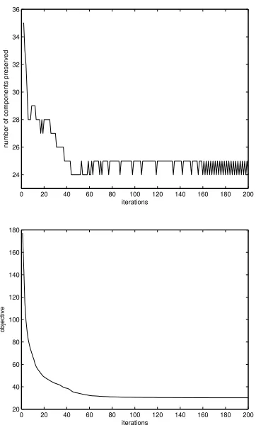
It is also interesting to inspect the numbers of principal components used by the PNAT updates (33). We kept the principal components of natural gradients such that the square root sum of the preserved eigenvalues exceeds 95%
of the total. The numbers of components in the first 200 iterations are plotted in Figure 5 (top). First we can see that all the numbers are far less than 66, the dimensionality of the gradients while preserving most of the direction information. This verifies the existence of principal variance of gradient vectors. Next, the learning requires more components at the beginning when the model parameters are random and less components in the subsequent iterations. Finally the number becomes stable between 24 and 25. The zoomed
−20 −15 −10 −5 0 5 10 15 20 25
−20 −15 −10 −5 0 5 10 15 20 25
dimension 1
dimension 2
bad good
−15 −10 −5 0 5 10 15 20 25
−15 −10 −5 0 5 10 15 20 25
dimension 1
dimension 2
bad good
Fig. 4. Ionosphere data in the projected space. Top: 1,000 natural gradient updates with η = 3×10⁻⁴. Bottom: 1,000 PNAT updates withη = 3×10⁻³.
objective curve in the fist 200 iterations is also displayed in Figure 5 (bottom) for alignment. It is easy to see that the changing trend of the number of principal components is well consistent with the objective convergence.
V. CONCLUSIONS
0 20 40 60 80 100 120 140 160 180 200 24
26 28 30 32 34 36
iterations
number of components preserved
0 20 40 60 80 100 120 140 160 180 200 20
40 60 80 100 120 140 160 180
iterations
objective
Fig. 5. Top: The numbers of principal components used in the first 200 iterations. Bottom: The aligned objective curve.
has been validated by two simulations, one for recovering a Gaussian mixture model on artificial data and the other for learning a discriminative linear transformation on real ionosphere data.
The proposed approach can potentially be applied to higher-dimensional data such as images or text. Furthermore, adaptive learning in dynamic context may be achieved by adopting online Principal Component Analysis [14].
VI. ACKNOWLEDGEMENT
This work is supported by the Academy of Finland in the projects Neural methods in information retrieval based
on automatic content analysis and relevance feedback and
Finnish Centre of Excellence in Adaptive Informatics Re-search.
APPENDIX
We apply the induction method onrto prove Theorem 1. Whenr= 1, the number of columns of Ψis m. Therefore the column rank ofΨ, rankcol(Ψ), is obvious no greater than
m×r−r×(r−1)/2 =m.
Suppose rankcol(Ψ(k−1))≤m(k−1)−(k−1)(k−2)/2
holds forr=k−1,k∈Z+. Denotew(j)thej-th column of
W. Then we can write Ψ(k−1)= B(1), . . . ,B(k−1) with
block matrix representationB(j) which equals
f1x (1) 1
Pm
d=1x (1)
d w
(j)
d . . . f1x (1)
m Pmd=1x(1)d w(dj)
..
. . .. ...
fnx(1n)
Pm
d=1x
(n)
d w
(j)
d . . . fnx
(n)
m Pmd=1x(dn)wd(j)
.
(35) Now consider each of the matrices
˜
B(jk)≡B(j) B(k), j= 1, . . . , k−1. (36) Notice that the coefficients
ρ≡w(1k), . . . , w(mk),−w
(j)
1 , . . . ,−wm(j)
(37)
fulfill
ρTB˜(jk)= 0, j= 1, . . . , k−1. (38) Treating the columns as symbolic objects, one can solve the
k−1 equations (38) by for example Gaussian elimination and then write out the last k−1columns of Ψ(k)as linear combinations of the first mr−(k−1) columns. That is, at most m−(k−1) linearly independent dimensions can be added whenw(k)is appended. The resulting column rank of
Ψ(k) is therefore no greater than
m(k−1)−(k−1)(k−2)
2 +m−(k−1) =mk−
k(k−1) 2 .
(39)
REFERENCES
[1] S. Amari. Natural gradient works efficiently in learning. Neural Computation, 10(2):251–276, 1998.
[2] S. Amari and H. Nagaoka. Methods of information geometry. Oxford University Press, 2000.
[3] S. Amari, H. Park, and K. Fukumizu. Adaptive method of realizing natural gradient learning for multilayer perceptrons. Neural Compu-tation, 12(6):1399–1409, 2000.
[4] C.L. Blake D.J. Newman, S. Hettich and C.J. Merz. UCI repository of machine learning databases http://www.ics.uci.edu/∼mlearn/MLRepository.html, 1998.
[5] J. Goldberger, S. Roweis, G. Hinton, and R. Salakhutdinov. Neigh-bourhood components analysis. Advances in Neural Information Processing, 17:513–520, 2005.
[6] Gene H. Golub and Charles F. van Loan. Matrix Computations. The Johns Hopkins University Press, 2 edition, 1989.
[7] A. Hyv¨arinen and P. Hoyer. Emergence of phase- and shift- invariant features by decomposition of natural images into independent feature subspaces.Neural Computation, 12(7):1705–1720, 2000.
[8] Y. Nishimori and S. Akaho. Learning algorithms utilizing quasi-geodesic flows on the Stiefel manifold.Neurocomputing, 67:106–135, 2005.
[9] J. Peltonen and S. Kaski. Discriminative components of data. IEEE Transactions on Neural Networks, 16(1):68–83, 2005.
[10] P. Peterson. Riemannian geometry. Springer, New York, 1998. [11] C. R. Rao. Information and accuracy attainable in the estimation of
statistical parameters. Bulletin of the Calcutta Mathematical Society, 37:81–91, 1945.
[12] J. S¨arel¨a and H. Valpola. Denoising source separation. Journal of Machine Learning Research, 6:233–272, 2005.
[13] W. Wan. Implementing online natural gradient learning: problems and solutions. IEEE Transactions on Neural Networks, 17(2):317–329, 2006.
[14] B. Yang. Projection approximation subspace tracking. IEEE Transac-tions on Signal Processing, 43(1):95–107, 1995.