OPTIMUM TILT ANGLE AND NEAR SHADING ANALYSIS FOR 1000 WATT PEAK PHOTOVOLTAIC APPLICATION SYSTEM

(1)

Seminar Nasional Sains dan Teknologi 2018 1 Fakultas Teknik Universitas Muhammadiyah Jakarta , 17 Oktober 2018

OPTIMUM TILT ANGLE AND NEAR SHADING ANALYSIS FOR 1000

WATT PEAK PHOTOVOLTAIC APPLICATION SYSTEM

Handoko Rusiana Iskandar, Zul Fakhri

Electrical Engineering Departement, Faculty of Engineering, Universitas Jenderal Achmad Yani. Jalan Terusan Jenderal Sudirman PO BOX 148, Cimahi, West Java, Indonesia. 40521.

E-mail: [email protected]

Abstrak

Teknologi pemanfaatan energi matahari mengalami peningkatan dan berperan peran penting dalam mendukung kebutuhan energi di masa depan sehingga mampu didistribusikan secara luas. Dalam tulisan ini penentuan sudut kemiringan atau tilt angle yang optimal dan sudut azimuth optimal panel photovoltaic, menggunakan PVSyst simulation software. Studi ini didasarkan nilai radiasi matahari global dan temperatur permukaan horizontal. Sudut kemiringan optimal untuk setiap bulan memungkinkan kita untuk mengumpulkan energi matahari maksimum pertahun. Hasil pemodelan yang dilakukan pada sistem PLTS 1000 Wp di lintang 6˚53'2.69"S dan bujur 107˚32'28.69", menghasilkan kerugian rata-rata 0.6%, dan global irradiance

yang mampu diserap oleh panel surya adalah 1747 kWh/m2_{pertahun dengan sudut}

kemiringan panel surya 15˚. Hasil simulasi faktor near shading menunjukkan faktor bayangan pada luas daerah yang diarsir setiap modul surya adalah 0.68 m2_.

Kata kunci: Azimuth, global irradiance, near shading, photovoltaic, tilt angle.

Abstract

The technology of solar energy utilization has increased and has an important role in supporting energy needs in the future so that it can be widely distributed. In this paper determine the optimal tilt angle and optimal azimuth angle of the photovoltaic panel, using PVSyst simulation software. The study is based on the value of global solar radiation and horizontal surface temperature. The optimal tilt angle for each month allows us to collect maximum solar energy per year. The modeling results performed on a 1000 Wp photovoltaic system at the latitude of 6˚53'2.69 "S and longitude 107˚ 32'28.69", resulted in an average loss of 0.6%, and the global irradiance capable of being absorbed by solar panels was 1747 kWh/m2_{per year with the angle of solar panel}

15˚. Near shading simulation result from the showing a shading factor from the simulation of the construction of PV system, the result of shaded areas per module area is 0.68 m2_.

Keywords: Azimuth, global irradiance, near shading, photovoltaic, tilt angle.

PENDAHULUAN

With the limitations of fossil energy sources, high fuel prices, and an abundance of new renewable energy resources, the government needs to develop new and renewable energy to meet electricity needs (Sangwongwanich, 2014). One of the most renewable sources of renewable energy developed is solar power plants that utilize solar energy. Nowadays, Interest in the utilization of renewable energy, especially solar energy more

than other new energy because the installation is easy and at a low cost (Iskandar, Purwadi, Rizqiawan, & Heryana, 2016)

(2)

percentage of efficiency. The characteristics of solar cells can be seen in the I-V curve which determines the amount of short circuit current (ISC), open circuit voltage (VOC) and several other

factors that influence the characteristics of solar cells.

In addition to decreasing the power of the solar panel caused by the calculation of direct current conductor cable as already done by (Iskandar, Rizqiawan, & Heryana, 2015), which explains some calculation techniques easily and the suitability of voltage drop in the permitted conductor, the effect of the output power on the solar panel is also examined by (Panchula, 2011) is about calculating energy loss losses on solar cell panels. Similarly, the study of the effect of temperature on the surface of solar cells on (Heriyanto, 2011), resulting in a rise in temperature causing the open circuit voltage (VOC) to decrease, but the short circuit current

(ISC) increases. The effect of temperature on the

voltage and electric current produced by solar cells is also affected by the level of sunlight intensity and the air temperature of the environment. The lower the radiation intensity of sunlight, the lower the current and the resulting light. Environmental temperature around solar panels also has a contribution to temperature changes in the performance of solar cells. Due to the increase in temperature, the voltage produced by the solar panel becomes incompatible with the nominal voltage (Suryana & Ali, 2016).

The photovoltaic system will work on its nominal voltage by maximizing the angle and reducing the shadow effect on the solar panel. Several studies and studies have been carried out and related to characteristic analysis of I - V curves, as well as maximum photovoltaic power modeling related to shading effects on output power, including reduction in power output due to deteriorating hot spots on the panels placed in the shade. To understand the partial shading phenomenon, the PV panel output levels are analyzed with various types of shading patterns and various environmental conditions (Bharadwaj & John, 2017).

The proposed sub-cell based method proved to provide the least error when compared with experimental measurements. This shows that the proposed modeling approach increases accuracy by 5 – 10% compared to the average insolation based modeling approach.

An analysis of the shading effect on the circuit to reduce losses caused by partial shading is carried out by (Srinivasa Rao, Saravana Ilango, & Nagamani, 2014). Modeling results using MATLAB show that the power taken from the PV array in partial shading conditions increases. Another method for detecting errors that occur between PV modules. Various errors will occur such as voltage (VOC), short circuit

(ISC) and error detection in shady conditions,

normal conditions and partial shadows. ANN is used to detect errors that occur on or between PV modules in normal and partial shading conditions and tested with random input carried out by (Kumar & Selvakumar, 2017). PV performance is influenced by temperature, solar radiation, shading, and array configuration. In research (Laamami, Benhamed, & Sbita, 2017) to optimize the performance of a PV system, it must initially lead to the efficiency of the PV system, then a global analysis of the characteristics of I-V from the PV module. Furthermore, an array model of solar cells is modeled to study the characteristics of I-V from PV modules under changes in external solar radiation. However, the P-V characteristics of PV are more complex with a lot of MPP under Partially Shad Condition. Parallel off-line tracking function is introduced to improve FMPPT performance. The results show that the enhanced FMPPT has better performance against the effect of partial shading because it can control the array operating voltage to adapt outside the local MPP. As a result the model approach using Fuzzy can increase the Maximum Power Point Tracker even though the PLTS power characteristics are influenced by the shading effect (Chin, Neelakantan, Yoong, Yang, & Teo, 2011).

(3)

Figure 2. Equivalent circuit of the modules

Table 1. Specification of PV module

No. Parameters Info.

1. Max. Op. Voltage (𝑉_𝑚𝑝_𝑚𝑎𝑥) 18 V

2. Max. Op. Current (𝐼_𝑚𝑝_𝑚𝑎𝑥_.) 5.56 A

3. Short Circuit Current (𝐼_𝑆𝐶) 6.02 A

4. Temp. Coefficient of 𝑃_𝑚𝑎𝑥 (%)

-0.47/℃

METODE

Characteristics of Solar Cell

The first step is to model the characteristics of solar cells. As a power source of the system, a PV array is considered one of the most important components. A PV array consists of several PV modules, and a PV module itself consists of a number of PV cells to satisfy current and/or voltage requirements. PV cells are a basic structure with high modularity(Iskandar, Zainal, & Purwadi, 2017). Therefore, PV cell models can describe the characteristics of PV arrays and PV modules.

Figure 2 shows the standard equivalent circuit for solar cells is a circuit model consisting of 1 diode. A constant source for photo-generated current (𝑖_𝑜), series resistance (𝑅_𝑠) and parallel constraints (𝑅_𝑠ℎ). Therefore, equation for the current (I) and the voltage (V) described by the equation as shown in (1).

𝑖𝑝𝑣 = 𝑖𝑝ℎ− 𝑖𝑜[𝑒𝑥𝑝 (𝑣_𝑛𝑘𝑝𝑣+𝑖_𝐵_{𝑇 𝑞}𝑝𝑣_⁄𝑅𝑠) − 1] −

𝑣𝑝𝑣+𝑖𝑝𝑣𝑅𝑠

𝑅𝑝 (1)

The equation (1), k is the Boltzman constant (1.3806503 × 10-23 J/K), T is cell’s operating temperature in degree Kelvin and q is the electron charge (1.60217646 × 10-19 C). where I is the terminal current of the solar cell, IPV is the light-generated current of solar cell,

V is the solar cell terminal voltage, RS is the

equivalent series resistance and RP is the

equivalent parallel resistance. The solar power generation system in this paper consists of a PV array of 10 series-connected modules; each module is composed of 36 cells. The equation of Photo-current as a function of temperature and irradiation be given by the equation (2).

𝐼𝑃𝑉= _𝐺𝐺_𝑛[𝐼𝑃𝑉.𝑛+ ∆𝐼𝑆𝐶 (𝑇𝑐− 𝑇𝑛)] (2)

(4)

Figure 3. Location of PV plant

START and PV characteristics are met

in the system

Figure 4. Flowchart for optimum design

Location and Geographical

The second step is determining the geographical location. In this research, 1000 Watt peak PV system will be applied in the Electrical Engineering Laboratory, General Achmad Yani University, Cimahi, West java,

Indonesia. Based on NASA Surface

Meteorology & Solar Energy the location of this solar insolation in kWh/m2_{/day, average air}

temperature at altitude of 10 m above ground level in ℃, and average relative humidity in %

at a latitude of 6°53'2.69"S and a longitude of 107°32'28.69"E as shown in figure 3.

Table 2. Yearly climate information

Month

Table 2 horizontal surface monthly in one year is 4.81 kWh/m2_{/day, average air}

temperature at altitude of 10 m above ground level is 26.99℃, and average relative humidity is 81.3 %.

Tilt Angle Calculation

(5)

Figure 5. Calculation of angle on solar panel

Figure 5 show to define the sun position given by time function, latitude and longitude and then used to calculate the size and position of the shading area. The altitudeof the Sun as PV cell is following equation (4)

cos 𝜃 = 𝑐𝑜𝑠𝛿 cos 𝜔 (cos 𝛾 sin 𝛽 sin₊

From the (Guo et al., 2017) according to the “radiation-maximized” demand and the mathematical model of solar obit and position Equation (6) reflects the optimization problem, in which the tilt angle and azimuth angle are

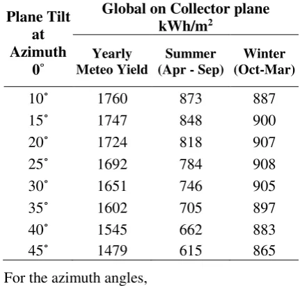
Table 3. Yearly data with various tilt angle

Plane Tilt 107°32'28.69"E. The most energy produced in the average per year is at the slope angles of 20˚, 15˚ and 10˚. The global value on collector plane >1700 kWh/m2_{with consideration of the}

standard test condition (STC), namely solar

irradiance 1000 W/m2_{and temperature 25}˚_C.

Module temperature calculation

The solar module changes the difference in energy carried by photons and the band gap of silicon into heat rather than converting them into electrical energy. The amount of photon energy absorbed will exceed the energy band, so the electrons which absorb photon energy will excite to the lowest band conduction level, causing a heat loss. The equation (9) is the calculation of the module output power from the results of multiplication between the power of the module and derating factor.

𝑃𝑚𝑜𝑑= 𝑃𝑆𝑇𝐶𝑥𝑓𝑚𝑎𝑛𝑥𝑓𝑡𝑒𝑚𝑝𝑥𝑓𝑑𝑖𝑟𝑡 (9)

Where 𝑃_𝑚𝑜𝑑 is derated power output in

Watt,𝑃_𝑆𝑇𝐶 is nominal output power on standard

(6)

is decreasing factor due to dust (Clean 1.0, Low 0.98, Medium 0.97, High 0.92). Determination of the factor of decrease due to temperature can be determined by the following equation (10),

𝑓𝑡𝑒𝑚𝑝= 1 − 𝛾 (𝑇𝑐𝑒𝑙𝑙,𝑒𝑓𝑓− 𝑇𝑆𝑇𝐶)

(10)

Where γ is the air temperature coefficient (%/℃), and 𝑇_{𝑐𝑒𝑙𝑙,𝑒𝑓𝑓} is the average effective temperature of solar cell. According to the nameplate module, the solar panel temperature coefficient has -0.47%/℃ at maximum power. Generally, silicone crystalline type modules have -0.4 to -0.5%/℃ (see table 1).

Photovoltaic Configuration

Installation of power plants with solar power requires planning regarding the power requirements used. To calculate the number of electrical energy needs is to multiply the amount of power and time of ignition. From the calculation of daily use equipment, the daily load requirement is obtained,

𝑃 = 𝑊 . 𝑡 (𝑤ℎ) (11) Calculation of the total operating voltage and current depends on the configuration of the solar installed in series, parallel, or parallel-series modules, solar installed in parallel-series shown by equation (12) and (13).

𝑉𝑚𝑝𝑡𝑜𝑡𝑎𝑙−𝑠𝑒𝑟𝑖= ∑ = 1 𝑉𝑖𝑛 𝑚𝑝_𝑛 (12) 𝐼𝑚𝑝𝑡𝑜𝑡𝑎𝑙−𝑠𝑒𝑟𝑖 = 𝐼𝑚𝑝_𝑛 (13)

In the solar configuration in parallel module, shown by equation (14) and (15).

𝑉𝑚𝑝𝑡𝑜𝑡𝑎𝑙−𝑝𝑎𝑟𝑎𝑙𝑒𝑙 = 𝑉𝑚𝑝_𝑛 (14) 𝐼𝑚𝑝𝑡𝑜𝑡𝑎𝑙−𝑝𝑎𝑟𝑎𝑙𝑒𝑙 = ∑ = 1 𝐼𝑖𝑛 𝑚𝑝_𝑛 (15)

Solar module configuration in series-parallel, shown by equation (16) and (17).

𝑉𝑚𝑝𝑡𝑜𝑡𝑎𝑙_𝑠𝑒𝑟𝑖+𝑝𝑎𝑟𝑎𝑙𝑒𝑙 = 𝑉𝑚𝑝_𝑡𝑜𝑡𝑎𝑙_𝑠𝑒𝑟𝑖 (16) 𝐼𝑚𝑝_{𝑡𝑜𝑡𝑎𝑠𝑒𝑟𝑖+𝑝𝑎𝑟𝑎𝑙𝑒𝑙} = ∑ = 1 𝐼𝑖𝑛 𝑚𝑝𝑡𝑜𝑡𝑎𝑙_𝑠𝑒𝑟𝑖 (17)

From the equation (16) and (17) are the voltages and currents in the maximum power of the series of modules arranged in series and parallel combinations. 𝑃_𝑚𝑝 is the maximum power that can be produced by the PV system,

𝑉𝑚𝑝 and 𝐼𝑚𝑝 are voltage and current at

maximum power, shown by equation (18).

𝑃𝑚𝑝= 𝑉𝑚𝑝𝐼𝑚𝑝

(18)

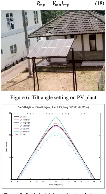
Figure 6. Tilt angle setting on PV plant

Figure 7. Sun’s height˚ to solar time in hours

RESULT AND DISCUSSION

Modeling of Solar Cell

Figure 6 shows the PV angle on 1000 Watt peak in Electrical Engineering Laboratory, General Achmad Yani University. Base on the table 1 the calculation result by the equation (12) has maximum operating voltage (𝑉_𝑚𝑝) 18 Volts, an open circuit voltage (𝑉_𝑂𝐶) is 22.36 V and the sum of voltage for 10 solar panels of 180 V and the power maximum is 1008 Watt.

Figure 7 shows potential energy in sun peak hours in one year. Base on location of the PV plant the most peak power performance in September and July, with a number of sun peak hours, of course, will affect the amount of energy that will be received by the solar cell module on kWh/m2 _{see in table 2. In this study,}

(7)

component when the sun is hidden below the horizon.

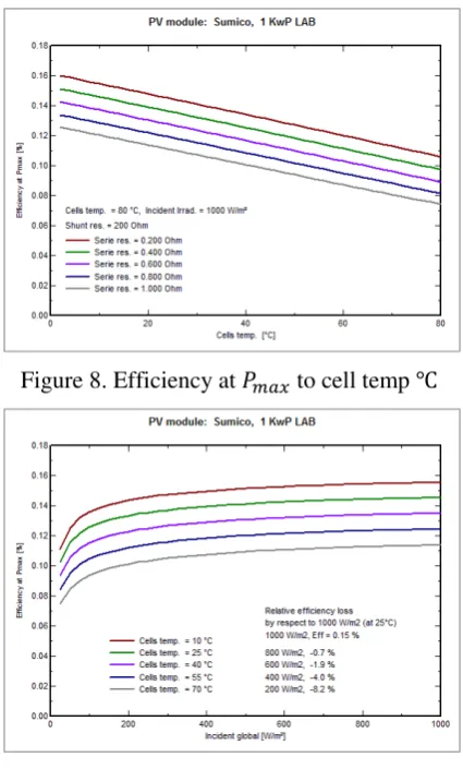
Figure 8. Efficiency at 𝑃_𝑚𝑎𝑥 to cell temp ℃

Figure 9. Eff. at 𝑃_𝑚𝑎𝑥to Inc. Global (W/m2₎

The temperature coefficient of the open circuit voltage 𝑚𝑢𝑉_𝑂𝐶 is normally determined by the program (one-diode model) during the choice of the series resistance. Nevertheless, it's variation's domain is restricted, and it is often hard to match the given value with an appropriate choice of 𝑅_𝑆.

Figure 8 shows the result efficiency at

𝑃𝑚𝑎𝑥 condition in 0.16%, the simulation in

PVsyst show the evaluation of the "Losses" of a PV array (as for the definition of the normalized performance ratio), takes as starting point the energy which would be produced if the system worked always at 𝑆_𝑇𝐶 condition (1000 W/m², 25°C). Figure 9 shows the performance cell in variant temperature 10℃, 25℃, 40℃, 55℃ and 70℃, if a high temperature in the cell indicates the efficiency will be lower, and the temperature in the cell is low, the efficiency will be higher. This graph shows the cells tested in various irradiance, high irradiance relative losses values will be better than the low

irradiance. Relative loss shows 0.7% at irradiance 800 W/m2_{compared to irradiance}

200 W/m2_{has a relative loss of 8.2%.}

Figure 10. I-V char. in various temperature

Figure 11. I-V char. in various irradiance

Figure 10 shows the results from simulation of the effect of temperature and Irradiance on the PV power characteristics of 1000 Watt peak, relationship 𝐼_𝑚𝑝 and 𝑉_𝑚𝑝on 1kWp PV, temperature variation on PV output power this simulation under Standard Test Condition.

(8)

In the one-diode model the two diodes are considered identical, and the Gamma factor - ranging theoretically from 1 to 2 - defines the mix between them.

Figure 12. Orientation on tilt 15˚ azimuth 0˚

Figure 13. Meteorology on plane tilt 15˚ azimuth 0˚ with shading (kWh/m2_.day)

Figure 14. Meteorology on plane tilt 15˚ azimuth 0˚ with shading (kWh/m2_.mth)

Figure 15. Mutual shading on plane tilt 15˚

Optimum Tilt Angle Analysis

The tilt angle has a large impact on solar radiation on the surface of the solar module. For a fixed tilt angle. Maximum power for one year will be obtained when the tilt angle of the solar module is equal to the latitude of the location (see table 3). Mechanical systems in PV construction have a function to provide assurance in a PV and are arranged in such a way that the generating system can work efficiently, reliably and work in its optimum operation. Determining the angle of installation of solar panels is useful to justify facing the module towards the horizon.

Figure 12 shows tilt angle 15˚ chosen by the tilt angle in terms of annual work which results in better global collector plane kWh/m2_,

then specify the azimuth field remains at 0˚. This orientation result has 4.81 kWh/m2_{.day in}

global horizontal plane and 4.79 kWh/m2_{.day in}

global on tilt plane and 4.76 kWh/m2_{.day under}

the shading in one year as indicated by figure 13, and a while in figure 14 shows the meteorological data on monthly computation has 1757 kWh/m2_{.mth in global horizontal}

plane and 1747 kWh/m2_{.mth in global on tilt}

plane and 1737 kWh/m2_{.mth global with shed}

shading in one year. Monthly meteo computations is the quick meteo calculation for this site, and immediately estimate the irradiation losses over the year using PVsyst.

(9)

irradiance, i.e. the shading factor is the shaded area fraction of the full array. This also slightly depends on the number of sheds as the first one is not shaded. This call the "linear" shading. Therefore this calculation requires the specification of the number of strings in the transverse dimension of the shed, as well as the size of one cell.

Figure 15 shows the horizon is describing far shadings effects. This is the simplest way for defining shadings, but its use should be limited to obstacles distant of, say, twenty time the PV-array size.

Figure 16. Shading factor on tilt angle 15˚

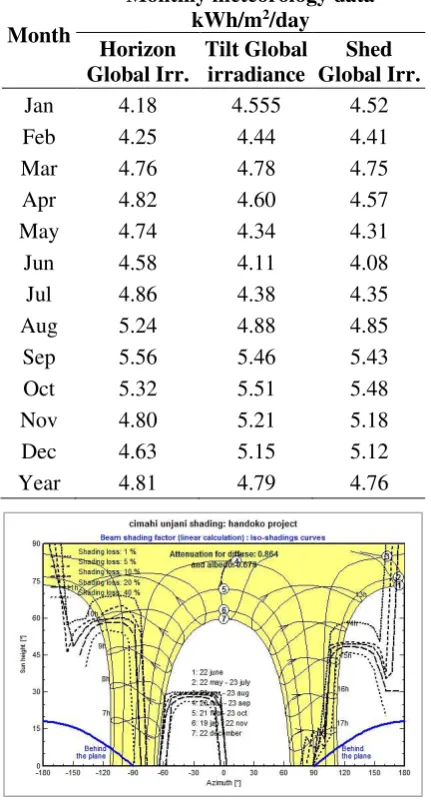
Table 4 shows the calculation result in monthly meteorological data using 15˚ and azimuth 0˚, where the global tilt plane average in one year is 4.79 kWh/m2_{/day and global}

under shading 4.76 kWh/m2_{/day. This table}

form usually includes the main parameters concerning the data, and for big tables (hourly or daily) choose by a desired period.

Near Shading Simulation Result

Figure 16 shows the sky diffuse component is also affected by the near shading obstacles. For simplification, we suppose that the diffuse sky irradiance is isotropic. At a given time, the shading effect on the diffuse irradiance can be thought as the integral of the shading factor over the visible part of the vault of heaven, that is the spherical dihedron between the collector plane and the horizontal plane. This is independent of the sun's position, and therefore constant over the year. The albedo is only visible from the collectors if no close obstacle is present till the level of the ground. This is the reason why we integrate the shading factor at zero height, over the portion of the sphere under the horizon, included between the horizontal plane and the plane of the collectors (below the ground). It is however to be remembered that for non-vertical planes, the energetic contribution of the albedo is weak in the global incident energy, and that errors in its estimation will therefore only have secondary repercussions. Spatial distribution of shadings on diffuse irradiation is smooth enough so that we can suppose that they don't affect the electrical behavior of the field. Therefore we will use the same diffuse and albedo shading factors for evaluating the shadings according to modules.

(10)

obstacle. The contribution should be null for near horizon, and up to 100% for a very distant one. The shading factor is applied to the beam component. This simulation has also calculated the shading factor for the diffuse component (as well as for the albedo), which is independent of the sun position and therefore constant over the year. Simulation results include shading loss calculations for Beam, Diffuse and Global irradiation components.

S

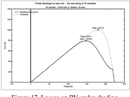
uperimposed on a sun's paths height/azimuth diagram, allowing to estimate at a glance the shading effects according to the season and time of day.

Figure 17. Losses on PV under shading

During simulation, the calculation of the shading factor for each hour would spend too much computing time. Therefore the programme establishes a table of shading factors as a function of the sun's height and azimuth. During simulation, the hourly shading factor can be calculated very fast by interpolation shown by the table 5. The table is a calculation of the shading factor (shaded fraction of the sensitive area, 1 = no shadings, 0 = full shaded), for all positions on the vault of heaven "seen" by your PV plane. It allows the calculation of the shading factor for the diffuse and albedo (which are integrals of this shading factor over the concerned spheric portion). At each hour, the simulation process will

interpolate in this table - according to the sun position - for evaluating the present shading factor on beam component. The geometric configuration of the shadow falling on the field, and the determination of the shading factor, are carried out in a purely geometric and analytical manner. For a given solar position, the programme first carries out a transformation of the coordinates of the whole system, so as to point the OZ' axis in the direction of the sun. Next, for each sensitive element of the PV fiel, it projects each elementary surface of the system on the plane of the field being considered. The shading loss factor is the ratio of the area of the shadow polygon, to that of the sensitive element. This process is repeated for each sensitive field element (for example each shed). This simulation, the calculation with a slightly different solar position (trials with modifications of 1° in height or azimuth). and, the shading factor is calculated in a completely different manner: the PV field is partitioned in about 2000 points, and the shading is calculated for each point. Although this method is an approximation, it always leads to a reliable result. In practice, this error has usually very little influence on the global simulation over one year. During the elaboration of the shading table, the points (sun's positions) situated behind the plane of the PV field appear in blue.

(11)

the collector plane (after taking irradiation shading effects into account), one can imagine that an ideal PV-array should yield 1 kilo Watt or kilo Watt peak under an irradiance of 1 kW. That is, assuming a linear response according to Irradiance, the ideal array will produce one kWh energy under one kWh irradiance for each installed kilo Watt peak (as defined at 𝑆_𝑇𝐶). The other parameters, the losses are about 20.8%, the 𝑃_𝑚𝑝𝑝 value will decrease to 792 W of

nominal power. This shows the

phenomenological study of the resultant I-V characteristic of a module or PV array, composed of non-identical cells or modules shows the partial shading curve between currents and voltages on one module. Cell area is the area of one cell, will give sensitive area of the module, and allow the definition of a solar cell production efficiency from the simulation of near shading the shading factor from the simulation of the construction of PV system, the result of shaded areas per module area is 0.68 m2_.

CONCLUSIONS

The modeling results performed on a 1000 Watt peak photovoltaic system at the latitude of 6˚53'2.69"S and longitude 107˚ 32'28.69", resulted in an average loss of 20.8%, and the calculation result in monthly meteorological data using 15˚ and azimuth 0˚, where the global tilt plane average in one year is 4.79 kWh/m2_{/day and global under shading}

4.76 kWh/m2_/day_{. Near shading simulation} result from the showing a shading factor from the simulation of the construction of PV system, the result of shaded areas per module area is 0.68 m2_{. The meteorological data on monthly}

computation has 1747 kWh/m2_{.mth in global on}

tilt plane and 1737 kWh/m2_{.mth global with}

shed shading in one year.

DAFTAR PUSTAKA

Bharadwaj, P., & John, V. (2017). Subcell Modelling of Partially Shaded Solar Photovoltaic Panels, 4406–4413.

Chin, C. S., Neelakantan, P., Yoong, H. P., Yang, S. S., & Teo, K. T. K. (2011). Maximum power point tracking for PV array under partially shaded conditions. In

Proceedings - 3rd International Conference on Computational Intelligence, Communication Systems and Networks, CICSyN 2011 (pp. 72–77).

Guo, M., Zang, H., Gao, S., Chen, T., Xiao, J., Cheng, L., … Sun, G. (2017). Optimal Tilt Angle and Orientation of Photovoltaic Modules Using HS Algorithm in Different Climates of China. Applied Sciences,

7(10), 1028.

Heriyanto, B. (2011). Pengaruh Suhu Permukaan Photovoltaic Module 50 Watt Peak Terhadap Daya Keluaran Yang Dihasilkan Menggunakan Reflektor Dengan Variasi Sudut Reflektor 0˚, 50˚, 60˚, 70˚, 80˚.Universitas Diponegoro. Iskandar, H. R., Purwadi, A., Rizqiawan, A., &

Heryana, N. (2016). Prototype

Development of a Low Cost Data Logger

and Monitoring System for PV

Application. In The 3rd IEEE Conference on Power Engineering and Renewable Energy (ICPERE) (pp. 171–177).

Iskandar, H. R., Rizqiawan, A., & Heryana, N. (2015). Perhitungan dan Penentuan Ukuran Kabel DC untuk Aplikasi Pembangkit Listrik Tenaga Surya. In

Seminar Nasional Ketenagalistrikan dan Aplikasinya (SENKA).

Iskandar, H. R., Zainal, Y. B., & Purwadi, A. (2017). Studi Karakteristik Kurva I-V dan P-V pada Sistem PLTS Terhubung Jaringan PLN Satu Fasa 220 VAC 50 HZ menggunakan Tracking DC Logger dan Low Cost Monitoring System. In Seminar Nasional Penerapan Ipteks Menuju Industri Masa Depan (PIMIMD-4) (pp. 174–183).

Kumar, S., & Selvakumar, A. (2017). Detection of the faults in the photovoltaic array under normal and partial shading conditions. International Conference on Innovations in Power and Advanced Computing Technologies, 1–5.

Laamami, S., Benhamed, M., & Sbita, L. (2017). Analysis of shading effects on a photovoltaic array. International Conference on Green Energy and Conversion Systems, GECS 2017. Panchula, A. F. (2011). Practical calculation of

lost energy for large PV power plants.

Conference Record of the IEEE Photovoltaic Specialists Conference, (3), 002412–002414.

(12)

Sangwongwanich, A. (2014). A New Power Control Strategy for Grid-Friendly Single-Phase Photovoltaic Systems. Srinivasa Rao, P., Saravana Ilango, G., &

Nagamani, C. (2014). Maximum power from PV arrays using a fixed configuration under different shading

conditions. IEEE Journal of

Photovoltaics, 4(2), 679–686.