OVERVIEW
In Chapter 2, we defined the slope of a curve at a point as the limit of secant
slopes. This limit, called a derivative, measures the rate at which a function changes, and it
is one of the most important ideas in calculus. Derivatives are used to calculate velocity
and acceleration, to estimate the rate of spread of a disease, to set levels of production so
as to maximize efficiency, to find the best dimensions of a cylindrical can, to find the age
of a prehistoric artifact, and for many other applications. In this chapter, we develop
tech-niques to calculate derivatives easily and learn how to use derivatives to approximate
com-plicated functions.
D
IFFERENTIATION
3
The Derivative as a Function
At the end of Chapter 2, we defined the slope of a curve
at the point where
to be
We called this limit, when it existed, the derivative of ƒ at
We now investigate the
derivative as a function
derived from ƒ by considering the limit at each point of the
do-main of ƒ.
x
0.
lim
h:0
ƒsx
0+
hd
-
ƒsx
0d
h
.
x
=
x
0y
=
ƒsxd
3.1
H
ISTORICALE
SSAY The DerivativeDEFINITION
Derivative Function
The
derivative
of the function ƒ(x) with respect to the variable x
is the function
whose value at x
is
provided the limit exists.
ƒ
¿
sxd
=
lim
h:0
ƒsx
+
hd
-
ƒsxd
h
,
We use the notation ƒ(x) rather than simply ƒ in the definition to emphasize the
inde-pendent variable x, which we are differentiating with respect to. The domain of
is the set
of points in the domain of ƒ for which the limit exists, and the domain may be the same or
smaller than the domain of ƒ. If
exists at a particular x, we say that ƒ is
differentiable
(has a derivative)
at x. If
exists at every point in the domain of ƒ, we call ƒ
differen-tiable
.
If we write
then
and h
approaches 0 if and only if z
approaches
x. Therefore, an equivalent definition of the derivative is as follows (see Figure 3.1).
h
=
z
-
x
z
=
x
+
h,
ƒ
¿
ƒ
¿
ƒ
¿
Alternative Formula for the Derivative
ƒ
¿
sxd
=
lim
z:x
ƒszd
-
ƒsxd
z
-
x
.
Calculating Derivatives from the Definition
The process of calculating a derivative is called
differentiation
. To emphasize the idea
that differentiation is an operation performed on a function
we use the notation
as another way to denote the derivative
Examples 2 and 3 of Section 2.7 illustrate
the differentiation process for the functions
and
Example 2 shows
that
For instance,
In Example 3, we see that
Here are two more examples.
EXAMPLE 1
Applying the Definition
Differentiate
Solution
Here we have ƒsxd
=
x
x
-
1
ƒsxd
=
x
x
-
1
.
d
dx
a
1
x
b
= -
x
1
2.
d
dx
a
3
2
x
-
4
b
=
3
2
.
d
dx
smx
+
bd
=
m.
y
=
1
>
x.
y
=
mx
+
b
ƒ
¿
sxd
.
d
dx
ƒsxd
y
=
ƒsxd,
x z
h z x P(x, f(x))
Q(z, f(z))
f(z) f(x) y f(x)
Secant slope is f(z) f(x)
z x
Derivative of f at x is f '(x) lim
h→0
lim
z→x
f(x h) f(x) h
f(z) f(x) z x
FIGURE 3.1 The way we write the
and
EXAMPLE 2
Derivative of the Square Root Function
(a)
Find the derivative of
for
(b)
Find the tangent line to the curve
at
Solution
(a)
We use the equivalent form to calculate
(b)
The slope of the curve at
is
The tangent is the line through the point (4, 2) with slope
(Figure 3.2):
We consider the derivative of
y
=
1
x
when
x
=
0
in Example 6.
You will often need to know the derivative of for
d
FIGURE 3.2 The curve and its
tangent at (4, 2). The tangent’s slope is found by evaluating the derivative at (Example 2).
Notations
There are many ways to denote the derivative of a function
where the
independ-ent variable is x
and the dependent variable is y. Some common alternative notations for
the derivative are
The symbols
and D
indicate the operation of differentiation and are called
differentiation operators
. We read
as “the derivative of y
with respect to x,” and
and (
)ƒ(x) as “the derivative of ƒ with respect to x.” The “prime” notations
and
come from notations that Newton used for derivatives. The
notations are
simi-lar to those used by Leibniz. The symbol
should not be regarded as a ratio (until we
introduce the idea of “differentials” in Section 3.8).
Be careful not to confuse the notation D(ƒ) as meaning the domain of the function ƒ
instead of the derivative function
The distinction should be clear from the context.
To indicate the value of a derivative at a specified number
we use the notation
For instance, in Example 2b we could write
To evaluate an expression, we sometimes use the right bracket ] in place of the vertical bar
Graphing the Derivative
We can often make a reasonable plot of the derivative of
by estimating the slopes
on the graph of ƒ. That is, we plot the points
in the xy-plane and connect them
with a smooth curve, which represents
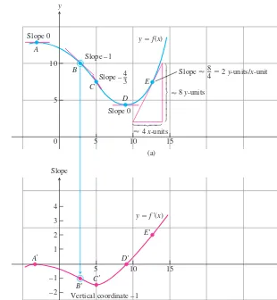
EXAMPLE 3
Graphing a Derivative
Graph the derivative of the function
in Figure 3.3a.
Solution
We sketch the tangents to the graph of ƒ at frequent intervals and use their
slopes to estimate the values of
at these points. We plot the corresponding
pairs and connect them with a smooth curve as sketched in Figure 3.3b.
What can we learn from the graph of
At a glance we can see
1.
where the rate of change of ƒ is positive, negative, or zero;
2.
the rough size of the growth rate at any x
and its size in relation to the size of ƒ(x);
3.
where the rate of change itself is increasing or decreasing.
Here’s another example.
EXAMPLE 4
Concentration of Blood Sugar
On April 23, 1988, the human-powered airplane Daedalus
flew a record-breaking 119 km
from Crete to the island of Santorini in the Aegean Sea, southeast of mainland Greece.
Dur-y
=
ƒ
¿
sxd?
sx, ƒ
¿
sxdd
ƒ
¿
sxd
y
=
ƒsxd
y
=
ƒ
¿
sxd
.
sx, ƒ
¿
sxdd
y
=
ƒsxd
ƒ
.
ƒ
¿
s4d
=
d
dx
1
x
`
x=4=
1
2
1
x
`
x=4=
1
2
2
4
=
1
4
.
ƒ
¿
sad
=
dy
dx
`
x=a=
df
dx
`
x=a=
d
dx
ƒsxd
`
x=a.
x
=
a,
ƒ
¿
.
dy
>
dx
d
>
dx
ƒ
¿
y
¿
d
>
dx
dƒ
>
dx
dy
>
dx
d
>
dx
ƒ
¿
sxd
=
y
¿ =
dy
dx
=
dƒ
dx
=
d
ing the 6-hour endurance tests before the flight, researchers monitored the prospective pilots’
blood-sugar concentrations. The concentration graph for one of the athlete-pilots is shown in
Figure 3.4a, where the concentration in milligrams deciliter is plotted against time in hours.
The graph consists of line segments connecting data points. The constant slope of
each segment gives an estimate of the derivative of the concentration between
measure-ments. We calculated the slope of each segment from the coordinate grid and plotted the
derivative as a step function in Figure 3.4b. To make the plot for the first hour, for
in-stance, we observed that the concentration increased from about 79 mg dL to 93 mg dL.
The net increase was
Dividing this by
gave
the rate of change as
Notice that we can make no estimate of the concentration’s rate of change at times
where the graph we have drawn for the concentration has a corner and no
slope. The derivative step function is not defined at these times.
t
=
1, 2,
Á
, 5 ,
¢
y
¢
t
=
14
1
=
14 mg
>
dL per hour .
¢
t
=
1 hour
¢
y
=
93
-
79
=
14 mg
>
dL .
>
>
>
0 10
(a)
5 15 x
5 10 Slope 0
A
B
C
D E
Slope 0
x 10
5 15
1 2 3 4
–1
– 2
(b) y
Slope –1
4 3 Slope –
y f(x)
Slope 8 2 y-units/x-unit 4
8 y-units
4 x-units
Slope
A'
y f '(x)
B' C'
D' E'
Vertical coordinate –1
FIGURE 3.3 We made the graph of in (b) by plotting slopes from the
graph of in (a). The vertical coordinate of is the slope at Band so on. The graph of ƒ¿is a visual record of how the slope of ƒ changes with x.
B¿
y = ƒsxd
Differentiable on an Interval; One-Sided Derivatives
A function
is
differentiable
on an open interval (finite or infinite) if it has a
de-rivative at each point of the interval. It is differentiable on a closed interval [a,
b] if it is
differentiable on the interior (a,
b) and if the limits
Right-hand derivative at
a
Left-hand derivative at
b
exist at the endpoints (Figure 3.5).
Right-hand and left-hand derivatives may be defined at any point of a function’s
do-main. The usual relation between one-sided and two-sided limits holds for these derivatives.
Because of Theorem 6, Section 2.4, a function has a derivative at a point if and only if it
has left-hand and right-hand derivatives there, and these one-sided derivatives are equal.
EXAMPLE 5
Is Not Differentiable at the Origin
Show that the function
is differentiable on
and
but has no
deriva-tive at
Solution
To the right of the origin,
To the left,
Rate of change of concentration,
mg
/dL h
FIGURE 3.4 (a) Graph of the sugar concentration in the blood of a Daedaluspilot
during a 6-hour preflight endurance test. (b) The derivative of the pilot’s blood-sugar concentration shows how rapidly the concentration rose and fell during various portions of the test.
FIGURE 3.5 Derivatives at endpoints are
one-sided limits.
Daedalus's flight path on April 23, 1988
(Figure 3.6). There can be no derivative at the origin because the one-sided derivatives
dif-fer there:
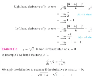
EXAMPLE 6
Is Not Differentiable at
In Example 2 we found that for
We apply the definition to examine if the derivative exists at
Since the (right-hand) limit is not finite, there is no derivative at
Since the slopes
of the secant lines joining the origin to the points
on a graph of
ap-proach
the graph has a vertical tangent
at the origin.
When Does a Function
Not
Have a Derivative at a Point?
A function has a derivative at a point
if the slopes of the secant lines through
and a nearby point Q
on the graph approach a limit as Q
approaches P.
When-ever the secants fail to take up a limiting position or become vertical as Q
approaches P,
the derivative does not exist. Thus differentiability is a “smoothness” condition on the
graph of ƒ. A function whose graph is otherwise smooth will fail to have a derivative at a
point for several reasons, such as at points where the graph has
1.
a corner, where the one-sided
2.
a cusp, where the slope of PQ
derivatives differ.
approaches
from one side and
from the other.
P
Q
Q P
Q Q
- q
q
Psx
0, ƒsx
0dd
x
0q
,
y
=
1
x
A
h,
1
h
B
x
=
0 .
lim
h:0+
2
0
+
h
-
2
0
h
=
hlim
:0+1
1
h
= q
.
x
=
0 :
d
dx
1
x
=
1
2
1
x
.
x
7
0 ,
x
=
0
y
=
1
x
=
lim
h:0-
-
1
= -
1 .
=
lim
h:0
--
h
h
Left-hand derivative of
ƒ
x
ƒ
at zero
=
lim
h:0
-ƒ
0
+
h
ƒ - ƒ
0
ƒ
h
=
hlim
:0-ƒ
h
ƒ
h
=
lim
h:0+
1
=
1
=
lim
h:0+
h
h
Right-hand derivative of
ƒ
x
ƒ
at zero
=
lim
h:0+
ƒ
0
+
h
ƒ - ƒ
0
ƒ
h
=
hlim
:0+ƒ
h
ƒ
h
x y
0
y' not defined at x 0: right-hand derivative
left-hand derivative
y' –1 y' 1
y x
FIGURE 3.6 The function is
not differentiable at the origin where the graph has a “corner.”
y = ƒxƒ
ƒhƒ =h when h 70 .
3.
a vertical tangent, where the slope of PQ
approaches
from both sides or
approaches
from both sides (here,
).
4.
a discontinuity.
Differentiable Functions Are Continuous
A function is continuous at every point where it has a derivative.
P
Q
Q
P
Q
Q
P Q
Q
- q
- q
q
THEOREM 1
Differentiability Implies Continuity
If ƒ has a derivative at
x
=
c
,
then ƒ is continuous at x
=
c.
Proof
Given that
exists, we must show that
or equivalently,
that If
then
=
ƒscd
+
ƒsc
+
hd
-
ƒscd
h
#
h.
ƒsc
+
hd
=
ƒscd
+
sƒsc
+
hd
-
ƒscdd
h
Z
0 ,
lim
h:0ƒsc
+
hd
=
ƒscd
.
lim
x:cƒsxd
=
ƒscd
,
Now take limits as
By Theorem 1 of Section 2.2,
Similar arguments with one-sided limits show that if ƒ has a derivative from one side
(right or left) at
then ƒ is continuous from that side at
Theorem 1 on page 154 says that if a function has a discontinuity at a point (for
in-stance, a jump discontinuity), then it cannot be differentiable there. The greatest integer
function fails to be differentiable at every integer
(Example
4,
Section 2.6).
CAUTION
The converse of Theorem 1 is false. A function need not have a derivative at a
point where it is continuous, as we saw in Example 5.
The Intermediate Value Property of Derivatives
Not every function can be some function’s derivative, as we see from the following theorem.
x
=
n
y
=
:
x
;
=
int
x
x
=
c.
x
=
c
=
ƒscd.
=
ƒscd
+
0
=
ƒscd
+
ƒ
¿
scd
#
0
lim
h:0
ƒsc
+
hd
=
hlim
:0ƒscd
+
hlim
:0ƒsc
+
hd
-
ƒscd
h
#
hlim
:0h
h
:
0 .
x y
0
1 y U(x)
FIGURE 3.7 The unit step
function does not have the Intermediate Value Property and cannot be the derivative of a function on the real line.
THEOREM 2
If a
and b
are any two points in an interval on which ƒ is differentiable, then
takes on every value between
ƒ
¿
sad
and ƒ
¿
sbd.
ƒ
¿
Theorem 2 (which we will not prove) says that a function cannot be
a derivative on an
in-terval unless it has the Intermediate Value Property there. For example, the unit step
func-tion in Figure 3.7 cannot be the derivative of any real-valued funcfunc-tion on the real line. In
Chapter 5 we will see that every continuous function is a derivative of some function.
EXERCISES 3.1
Finding Derivative Functions and Values
Using the definition, calculate the derivatives of the functions in Exer-cises 1–6. Then find the values of the derivatives as specified.
1.
2.
3. gstd = 1
t2 ; g¿s-1d, g¿s2d, g¿
A
23B
Fsxd = sx - 1d2 + 1; F¿s-1d, F¿s0d, F¿s2dƒsxd = 4 - x2; ƒ¿s-3d, ƒ¿s0d, ƒ¿s1d
4.
5.
6.
In Exercises 7–12, find the indicated derivatives.
7. 8. dr
ds if r = s3
2 + 1 dy
dx if y = 2x 3
rssd = 22s + 1 ; r¿s0d, r¿s1d, r¿s1>2d
psud = 23u ; p¿s1d, p¿s3d, p¿s2>3d
kszd = 1 - z
9.
10.
11.
12.
Slopes and Tangent Lines
In Exercises 13–16, differentiate the functions and find the slope of the tangent line at the given value of the independent variable.
13.
14.
15.
16.
In Exercises 17–18, differentiate the functions. Then find an equation of the tangent line at the indicated point on the graph of the function.
17.
18.
In Exercises 19–22, find the values of the derivatives.
19.
20.
21.
22.
Using the Alternative Formula for Derivatives
Use the formulato find the derivative of the functions in Exercises 23–26.
23.
Match the functions graphed in Exercises 27–30 with the derivatives graphed in the accompanying figures (a) – (d).
y'
31. a. The graph in the accompanying figure is made of line seg-ments joined end to end. At which points of the interval
b. Graph the derivative of ƒ.
The graph should show a step function.
32. Recovering a function from its derivative
a. Use the following information to graph the function ƒ over the closed interval
i) The graph of ƒ is made of closed line segments joined end to end.
ii) The graph starts at the point
iii)The derivative of ƒ is the step function in the figure shown here.
b. Repeat part (a) assuming that the graph starts at instead of
33. Growth in the economy The graph in the accompanying figure shows the average annual percentage change in the U.S. gross national product (GNP) for the years 1983–1988. Graph (where defined). (Source: Statistical Abstracts of the United States, 110th Edition, U.S. Department of Commerce, p. 427.)
34. Fruit flies (Continuation of Example 3, Section 2.1.) Popula-tions starting out in closed environments grow slowly at first, when there are relatively few members, then more rapidly as the number of reproducing individuals increases and resources are still abundant, then slowly again as the population reaches the carrying capacity of the environment.
a. Use the graphical technique of Example 3 to graph the derivative of the fruit fly population introduced in Section 2.1. The graph of the population is reproduced here.
1983 1984 1985 1986 1987 1988 0
b. During what days does the population seem to be increasing fastest? Slowest?
One-Sided Derivatives
Compare the right-hand and left-hand derivatives to show that the functions in Exercises 35–38 are not differentiable at the point P.
35. 36.
37. 38.
Differentiability and Continuity on an Interval
Each figure in Exercises 39–44 shows the graph of a function over a closed interval D. At what domain points does the function appear to bea. differentiable?
b. continuous but not differentiable?
c. neither continuous nor differentiable?
Give reasons for your answers.
a. Find the derivative of the given function
b. Graph and side by side using separate sets of
coordinate axes, and answer the following questions.
c. For what values of x, if any, is positive? Zero? Negative?
d. Over what intervals of x-values, if any, does the function increase as xincreases? Decrease as xincreases? How is this related to what you found in part (c)? (We will say more about this relationship in Chapter 4.)
45. 46.
47. 48.
49. Does the curve ever have a negative slope? If so, where? Give reasons for your answer.
50. Does the curve have any horizontal tangents? If so, where? Give reasons for your answer.
y = 21x
51. Tangent to a parabola Does the parabola
have a tangent whose slope is If so, find an equation for the line and the point of tangency. If not, why not?
52. Tangent to Does any tangent to the curve cross the x-axis at If so, find an equation for the line and the point of tangency. If not, why not?
53. Greatest integer in x Does any function differentiable on have the greatest integer in x(see Figure 2.55), as its derivative? Give reasons for your answer.
54. Derivative of Graph the derivative of Then
graph What can you conclude?
55. Derivative of Does knowing that a function ƒ(x) is differen-tiable at tell you anything about the differentiability of the function at Give reasons for your answer.
56. Derivative of multiples Does knowing that a function g(t) is differentiable at tell you anything about the differentiability of the function 3gat Give reasons for your answer.
57. Limit of a quotient Suppose that functions g(t) and h(t) are
defined for all values of t and Can
exist? If it does exist, must it equal zero? Give reasons for your answers.
58. a. Let ƒ(x) be a function satisfying for Show that ƒ is differentiable at and find
b. Show that
is differentiable at and find
59. Graph in a window that has Then, on
the same screen, graph
for Then try Explain what
is going on.
60. Graph in a window that has Then, on the same screen, graph
for Then try Explain what is
going on.
61. Weierstrass’s nowhere differentiable continuous function
The sum of the first eight terms of the Weierstrass function is
Graph this sum. Zoom in several times. How wiggly and bumpy is this graph? Specify a viewing window in which the displayed portion of the graph is smooth.
COMPUTER EXPLORATIONS
Use a CAS to perform the following steps for the functions in Exer-cises 62–67.
a. Plot to see that function’s global behavior.
b. Define the difference quotient qat a general point x, with general step size h.
c. Take the limit as What formula does this give?
d. Substitute the value and plot the function together with its tangent line at that point.
e. Substitute various values for xlarger and smaller than into the formula obtained in part (c). Do the numbers make sense with your picture?
x0 y = ƒsxd
x = x0 h:0 . y = ƒsxd
f. Graph the formula obtained in part (c). What does it mean when its values are negative? Zero? Positive? Does this make sense with your plot from part (a)? Give reasons for your answer.
62.
63.
64. 65.
66. ƒsxd = sin 2x, x0 = p>2 67. ƒsxd = x2 cos x, x0 = p>4
ƒsxd = x - 1
3x2 + 1, x0 = -1 ƒsxd = 4x
x2 + 1, x0 = 2 ƒsxd = x1>3+ x2>3, x0 = 1
Differentiation Rules
This section introduces a few rules that allow us to differentiate a great variety of
func-tions. By proving these rules here, we can differentiate functions without having to apply
the definition of the derivative each time.
Powers, Multiples, Sums, and Differences
The first rule of differentiation is that the derivative of every constant function is zero.
3.2
RULE 1
Derivative of a Constant Function
If ƒ has the constant value
then
dƒ
dx
=
d
dx
scd
=
0 .
ƒsxd
=
c,
EXAMPLE 1
If ƒ has the constant value
then
Similarly,
Proof of Rule 1
We apply the definition of derivative to
the function whose
outputs have the constant value c
(Figure 3.8). At every value of x, we find that
ƒ
¿
sxd
=
lim
h:0
ƒsx
+
hd
-
ƒsxd
h
=
hlim
:0c
-
c
h
=
hlim
:00
=
0 .
ƒsxd
=
c,
d
dx
a
-p
2
b
=
0
and
d
dx
a
2
3
b
=
0 .
df
dx
=
d
dx
s8d
=
0 .
ƒsxd
=
8 ,
x y
0 x
c
h
y c (x h, c) (x, c)
x h
FIGURE 3.8 The rule is
another way to say that the values of constant functions never change and that the slope of a horizontal line is zero at every point.
The second rule tells how to differentiate
x
nif n
is a positive integer.
RULE 2
Power Rule for Positive Integers
If n
is a positive integer, then
d
dx
x
n
=
nx
n-1.
To apply the Power Rule, we subtract 1 from the original exponent (n) and multiply
the result by n.
EXAMPLE 2
Interpreting Rule 2
ƒ
x
1
2x
First Proof of Rule 2
The formula
can be verified by multiplying out the right-hand side. Then from the alternative form for
the definition of the derivative,
Second Proof of Rule 2
If then
Since
n
is a positive
integer, we can expand
by the Binomial Theorem to get
The third rule says that when a differentiable function is multiplied by a constant, its
derivative is multiplied by the same constant.
=
nx
n-1=
lim
h:0
c
nx
n-1
+
nsn
-
1d
2
x
n-2
h
+ Á +
nxh
n-2+
h
n-1d
=
lim
h:0
nx
n-1h
+
nsn
-
1d
2
x
n-2
h
2+ Á +
nxh
n-1+
h
nh
=
lim
h:0
c
x
n+
nx
n-1h
+
nsn
-
1d
2
x
n-2
h
2+ Á +
nxh
n-1+
h
nd
-
x
nh
ƒ
¿
sxd
=
lim
h:0
ƒsx
+
hd
-
ƒsxd
h
=
hlim
:0sx
+
hd
n-
x
nh
sx
+
hd
nƒsx
+
hd
=
sx
+
hd
n.
ƒsxd
=
x
n,
=
nx
n-1=
lim
z:x
sz
n-1
+
z
n-2x
+ Á +
zx
n-2+
x
n-1d
ƒ
¿
sxd
=
lim
z:x
ƒszd
-
ƒsxd
z
-
x
=
zlim
:x
z
n-
x
nz
-
x
z
n-
x
n=
sz
-
xdsz
n-1+
z
n-2x
+ Á +
zx
n-2+
x
n-1d
Á
4x
33x
2ƒ
¿
Á
x
4x
3x
2H
ISTORICALB
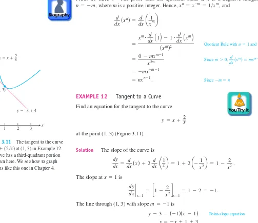
IOGRAPHY Richard CourantIn particular, if n
is a positive integer, then
EXAMPLE 3
(a)
The derivative formula
says that if we rescale the graph of
by multiplying each y-coordinate by 3,
then we multiply the slope at each point by 3 (Figure 3.9).
(b) A useful special case
The derivative of the negative of a differentiable function u
is the negative of the
func-tion’s derivative. Rule 3 with
gives
Proof of Rule 3
Limit property
uis differentiable
.
The next rule says that the derivative of the sum of two differentiable functions is the
sum of their derivatives.
=
c
du
dx
=
c
lim
h:0
usx
+
hd
-
usxd
h
d
dx
cu
=
hlim
:0cusx
+
hd
-
cusxd
h
d
dx
s
-
ud
=
d
dx
s
-
1
#
ud
= -
1
#
d
dx
sud
=
-du
dx
.
c
= -
1
y
=
x
2d
dx
s3x
2
d
=
3
#
2x
=
6x
d
dx
scx
n
d
=
cnx
n-1.
RULE 3
Constant Multiple Rule
If u
is a differentiable function of x, and c
is a constant, then
d
dx
scud
=
c
du
dx
.
RULE 4
Derivative Sum Rule
If u
and
y
are differentiable functions of x, then their sum
is differentiable
at every point where u
and
y
are both differentiable. At such points,
d
dx
su
+
y
d
=
du
dx
+
d
y
dx
.
u
+
y
x y
0 1
1
(1, 1)
2 2
3 (1, 3) Slope
Slope Slope 2x
2(1) 2 y x2 y 3x2
Slope 3(2x)
6x
6(1) 6
FIGURE 3.9 The graphs of and
Tripling the y-coordinates triples the slope (Example 3).
y = 3x2.
y = x2
Derivative definition with ƒsxd =cusxd
Denoting Functions by uand Y
EXAMPLE 4
Derivative of a Sum
Proof of Rule 4
We apply the definition of derivative to
Combining the Sum Rule with the Constant Multiple Rule gives the
Difference Rule,
which says that the derivative of a difference
of differentiable functions is the difference of
their derivatives.
The Sum Rule also extends to sums of more than two functions, as long as there are
only finitely many functions in the sum. If
are differentiable at x, then so is
and
EXAMPLE 5
Derivative of a Polynomial
Notice that we can differentiate any polynomial term by term, the way we
differenti-ated the polynomial in Example 5. All polynomials are differentiable everywhere.
Proof of the Sum Rule for Sums of More Than Two Functions
We prove the statement
by mathematical induction (see Appendix 1). The statement is true for
as was just
proved. This is Step 1 of the induction proof.
Step 2 is to show that if the statement is true for any positive integer
where
then it is also true for
So suppose that
(1)
Then
Eq. (1)
With these steps verified, the mathematical induction principle now guarantees the
Sum Rule for every integer
EXAMPLE 6
Finding Horizontal Tangents
Does the curve
have any horizontal tangents? If so, where?
Solution
The horizontal tangents, if any, occur where the slope
is zero. We have,
Now solve the equation
The curve
has horizontal tangents at
and
The
corre-sponding points on the curve are (0, 2), (1, 1) and
See Figure 3.10.
Products and Quotients
While the derivative of the sum of two functions is the sum of their derivatives, the
deriva-tive of the product of two functions is not
the product of their derivatives. For instance,
The derivative of a product of two functions is the sum of two
products, as we now explain.
d
FIGURE 3.10 The curve
and its horizontal tangents (Example 6).
y = x4 - 2x2 + 2
RULE 5
Derivative Product Rule
The derivative of the product u
y
is u
times the derivative of
y
plus
y
times the
deriva-tive of u. In prime notation,
In function notation,
EXAMPLE 7
Using the Product Rule
Find the derivative of
Solution
We apply the Product Rule with
and
Proof of Rule 5
To change this fraction into an equivalent one that contains difference quotients for the
de-rivatives of u
and
y
, we subtract and add
in the numerator:
As
h
approaches zero,
approaches
u(x) because
u, being differentiable at x, is
con-tinuous at x. The two fractions approach the values of
at x
and at
x. In short,
In the following example, we have only numerical values with which to work.
EXAMPLE 8
Derivative from Numerical Values
Let
be the product of the functions u
and
y
. Find
if
Solution
From the Product Rule, in the form
y
¿ =
su
y
d
¿ =
u
y
¿ +
y
u
¿
,
Example 3, Section 2.7. d Picturing the Product Rule
If u(x) and y(x) are positive and increase whenxincreases, and ifh 7 0 ,
0
then the total shaded area in the picture is
we have
EXAMPLE 9
Differentiating a Product in Two Ways
Find the derivative of
Solution(a)
From the Product Rule with
and
we find
(b)
This particular product can be differentiated as well (perhaps better) by multiplying
out the original expression for y
and differentiating the resulting polynomial:
This is in agreement with our first calculation.
Just as the derivative of the product of two differentiable functions is not the product of
their derivatives, the derivative of the quotient of two functions is not the quotient of their
derivatives. What happens instead is the Quotient Rule.
dy
dx
=
5x
4
+
3x
2+
6x.
y
=
sx
2+
1dsx
3+
3d
=
x
5+
x
3+
3x
2+
3
=
5x
4+
3x
2+
6x.
=
3x
4+
3x
2+
2x
4+
6x
d
dx
C A
x
2
+
1
B A
x
3+
3
B D
=
sx
2+
1ds3x
2d
+
sx
3+
3ds2xd
y
=
x
3+
3 ,
u
=
x
2+
1
y
=
sx
2+
1dsx
3+
3d.
=
s3ds2d
+
s1ds
-
4d
=
6
-
4
=
2 .
y
¿
s2d
=
us2d
y¿
s2d
+
y
s2du
¿
s2d
RULE 6
Derivative Quotient Rule
If u
and
y
are differentiable at x
and if
then the quotient
is
differ-entiable at x, and
d
dx
a
u
y
b
=
y
du
dx
-
u
d
y
dx
y
2.
u
>
y
y
sxd
Z
0 ,
In function notation,
EXAMPLE 10
Using the Quotient Rule
Find the derivative of
y
=
t
2-
1
t
2+
1
.
d
dx
c
ƒsxd
gsxd
d
=
Solution
We apply the Quotient Rule with
and
Proof of Rule 6
To change the last fraction into an equivalent one that contains the difference quotients for
the derivatives of u
and
y
, we subtract and add
y
(x)u(x) in the numerator. We then get
Taking the limit in the numerator and denominator now gives the Quotient Rule.
Negative Integer Powers of
x
The Power Rule for negative integers is the same as the rule for positive integers.
=
lim
h:0
y
sxd
usx
+
hd
-
usxd
h
-
usxd
y
sx
+
hd
-
y
sxd
h
y
sx
+
hd
y
sxd
.
d
dx
a
u
y
b
=
hlim
:0
y
sxdusx
+
hd
-
y
sxdusxd
+
y
sxdusxd
-
usxd
y
sx
+
hd
h
y
sx
+
hd
y
sxd
=
lim
h:0
y
sxdusx
+
hd
-
usxd
y
sx
+
hd
h
y
sx
+
hd
y
sxd
d
dx
a
u
y
b
=
hlim
:0
usx
+
hd
y
sx
+
hd
-usxd
y
sxd
h
=
4t
st
2+
1d
2.
=
2t
3+
2t
-
2t
3+
2t
st
2+
1d
2d
dt a
u
yb =
ysdu>dtd- usdy>dtd
y2
dy
dt
=
st
2+
1d
#
2t
-
st
2-
1d
#
2t
st
2+
1d
2y
=
t
2+
1 :
u
=
t
2-
1
RULE 7
Power Rule for Negative Integers
If n
is a negative integer and
then
d
dx
sx
n
d
=
nx
n-1.
x
Z
0 ,
EXAMPLE 11
(a)
Agrees with Example 3, Section 2.7(b)
d
dx
a
4
x
3b
=
4
d
dx
sx
-3
d
=
4s
-
3dx
-4= -
12
x
4d
dx
a
1
x
b
=
d
dx
sx
Proof of Rule 7
The proof uses the Quotient Rule. If n
is a negative integer, then
where m
is a positive integer. Hence,
and
Quotient Rule with and
Since
Since
EXAMPLE 12
Tangent to a Curve
Find an equation for the tangent to the curve
at the point (1, 3) (Figure 3.11).
Solution
The slope of the curve is
The slope at
is
The line through (1, 3) with slope
is
Point-slope equation
The choice of which rules to use in solving a differentiation problem can make a
dif-ference in how much work you have to do. Here is an example.
EXAMPLE 13
Choosing Which Rule to Use
Rather than using the Quotient Rule to find the derivative of
expand the numerator and divide by
y
=
sx
-
1dsx
FIGURE 3.11 The tangent to the curve
Then use the Sum and Power Rules:
Second- and Higher-Order Derivatives
If
is a differentiable function, then its derivative
is also a function. If
is
also differentiable, then we can differentiate
to get a new function of x
denoted by
So
The function
is called the
second derivative
of ƒ because it is the
deriv-ative of the first derivderiv-ative. Notationally,
The symbol
means the operation of differentiation is performed twice.
If
then
and we have
Thus
If
is differentiable, its derivative,
is the
third derivative
of y
with respect to x. The names continue as you imagine, with
denoting the
n
th derivative
of y
with respect to x
for any positive integer n.
We can interpret the second derivative as the rate of change of the slope of the tangent
to the graph of
at each point. You will see in the next chapter that the second
de-rivative reveals whether the graph bends upward or downward from the tangent line as we
move off the point of tangency. In the next section, we interpret both the second and third
derivatives in terms of motion along a straight line.
EXAMPLE 14
Finding Higher Derivatives
The first four derivatives of
are
First derivative:
Second derivative:
Third derivative:
Fourth derivative:
The function has derivatives of all orders, the fifth and later derivatives all being zero.
y
s4d=
0 .
How to Read the Symbols for Derivatives
“yprime” “ydouble prime” “dsquared y dxsquared” “ytriple prime”
EXERCISES 3.2
Derivative Calculations
In Exercises 1–12, find the first and second derivatives.
1. 2.
In Exercises 13–16, find (a) by applying the Product Rule and
(b)by multiplying the factors to produce a sum of simpler terms to differentiate.
13. 14.
15. 16.
Find the derivatives of the functions in Exercises 17–28.
17. 18.
Find the derivatives of all orders of the functions in Exercises 29 and 30.
29. 30.
Find the first and second derivatives of the functions in Exercises 31–38.
39. Suppose uand yare functions of xthat are differentiable at and that
Find the values of the following derivatives at
a. b. c. d.
40. Suppose uand yare differentiable functions of xand that
Find the values of the following derivatives at
a. b. c. d.
Slopes and Tangents
41. a. Normal to a curve Find an equation for the line perpendicular to the tangent to the curve at the point (2, 1).
b. Smallest slope What is the smallest slope on the curve? At what point on the curve does the curve have this slope?
c. Tangents having specified slope Find equations for the tangents to the curve at the points where the slope of the curve is 8.
42. a. Horizontal tangents Find equations for the horizontal
tan-gents to the curve Also find equations for
the lines that are perpendicular to these tangents at the points of tangency.
b. Smallest slope What is the smallest slope on the curve? At what point on the curve does the curve have this slope? Find an equation for the line that is perpendicular to the curve’s tangent at this point.
44. Find the tangent to the Witch of Agnesi(graphed here) at the point (2, 1).
45. Quadratic tangent to identity function The curve passes through the point (1, 2) and is tangent to the line at the origin. Find a,b, and c.
46. Quadratics having a common tangent The curves
and have a common tangent line at
the point (1, 0). Find a,b, and c.
47. a. Find an equation for the line that is tangent to the curve at the point
b. Graph the curve and tangent line together. The tangent intersects the curve at another point. Use Zoom and Trace to estimate the point’s coordinates.
c. Confirm your estimates of the coordinates of the second intersection point by solving the equations for the curve and tangent simultaneously (Solver key).
48. a. Find an equation for the line that is tangent to the curve at the origin.
b. Graph the curve and tangent together. The tangent intersects the curve at another point. Use Zoom and Trace to estimate the point’s coordinates.
c. Confirm your estimates of the coordinates of the second intersection point by solving the equations for the curve and tangent simultaneously (Solver key).
Theory and Examples
49. The general polynomial of degree nhas the form
where Find
50. The body’s reaction to medicine The reaction of the body to a dose of medicine can sometimes be represented by an equation of the form
where Cis a positive constant and Mis the amount of medicine absorbed in the blood. If the reaction is a change in blood pres-sure, Ris measured in millimeters of mercury. If the reaction is a change in temperature, Ris measured in degrees, and so on.
Find . This derivative, as a function of M, is called the sensitivity of the body to the medicine. In Section 4.5, we will see
dR>dM
how to find the amount of medicine to which the body is most sensitive.
51. Suppose that the function yin the Product Rule has a constant value c. What does the Product Rule then say? What does this say about the Constant Multiple Rule?
52. The Reciprocal Rule
a. The Reciprocal Rulesays that at any point where the function
y(x) is differentiable and different from zero,
Show that the Reciprocal Rule is a special case of the Quotient Rule.
b. Show that the Reciprocal Rule and the Product Rule together imply the Quotient Rule.
53. Generalizing the Product Rule The Product Rule gives the formula
for the derivative of the product uyof two differentiable functions of x.
a. What is the analogous formula for the derivative of the product uywof threedifferentiable functions of x?
b. What is the formula for the derivative of the product of fourdifferentiable functions of x?
c. What is the formula for the derivative of a product
of a finite number nof differentiable functions of x?
54. Rational Powers
a. Find by writing as and using the Product
Rule. Express your answer as a rational number times a rational power of x. Work parts (b) and (c) by a similar method.
b. Find
c. Find
d. What patterns do you see in your answers to parts (a), (b), and (c)? Rational powers are one of the topics in Section 3.6.
55. Cylinder pressure If gas in a cylinder is maintained at a con-stant temperature T, the pressure Pis related to the volume Vby a formula of the form
accompa-56. The best quantity to order One of the formulas for inventory management says that the average weekly cost of ordering, paying for, and holding merchandise is
where qis the quantity you order when things run low (shoes, ra-dios, brooms, or whatever the item might be); kis the cost of plac-ing an order (the same, no matter how often you order); cis the cost of one item (a constant); mis the number of items sold each week (a constant); and his the weekly holding cost per item (a constant that takes into account things such as space, utilities, in-surance, and security). Find dA>dqand d2A>dq2.
Asqd = kmq + cm+ hq
The Derivative as a Rate of Change
In Section 2.1, we initiated the study of average and instantaneous rates of change. In this
section, we continue our investigations of applications in which derivatives are used to
model the rates at which things change in the world around us. We revisit the study of
mo-tion along a line and examine other applicamo-tions.
It is natural to think of change as change with respect to time, but other variables can
be treated in the same way. For example, a physician may want to know how change in
dosage affects the body’s response to a drug. An economist may want to study how the cost
of producing steel varies with the number of tons produced.
Instantaneous Rates of Change
If we interpret the difference quotient
as the average rate of change
in ƒ over the interval from x
to
we can interpret its limit as
as the rate at
which ƒ is changing at the point x.
h
:
0
x
+
h,
sƒsx
+
hd
-
ƒsxdd
>
h
3.3
DEFINITION
Instantaneous Rate of Change
The
instantaneous rate of change
of ƒ with respect to x
at
is the derivative
provided the limit exists.
ƒ
¿
sx
0d
=
lim
h:0
ƒsx
0+
hd
-
ƒsx
0d
h
,
x
0Thus, instantaneous rates are limits of average rates.
EXAMPLE 1
How a Circle’s Area Changes with Its Diameter
The area A
of a circle is related to its diameter by the equation
How fast does the area change with respect to the diameter when the diameter is 10 m?
SolutionThe rate of change of the area with respect to the diameter is
When
the area is changing at rate
Motion Along a Line: Displacement, Velocity, Speed,
Acceleration, and Jerk
Suppose that an object is moving along a coordinate line (say an s-axis) so that we know
its position s
on that line as a function of time t:
The
displacement
of the object over the time interval from t
to (Figure 3.12)
is
and the
average velocity
of the object over that time interval is
To find the body’s velocity at the exact instant t, we take the limit of the average
ve-locity over the interval from t
to
as
shrinks to zero. This limit is the derivative of
ƒ with respect to t.
¢
t
t
+ ¢
t
y
ay=
displacement
travel time
=
¢
s
¢
t
=
ƒst
+ ¢
td
-
ƒstd
¢
t
.
¢
s
=
ƒst
+ ¢
td
-
ƒstd,
t
+ ¢
t
s
=
ƒstd
.
s
p
>
2d10
=
5
p
m
2>
m .
D
=
10 m ,
dA
dD
=
p
4
#
2D
=
p
D
2
.
A
=
p
4
D
2.
DEFINITION
Velocity
Velocity (instantaneous velocity)
is the derivative of position with respect to
time. If a body’s position at time t
is
then the body’s velocity at time t
is
y
std
=
ds
dt
=
¢lim
t:0ƒst
+ ¢
td
-
ƒstd
¢
t
.
s
=
ƒstd
,
EXAMPLE 2
Finding the Velocity of a Race Car
Figure 3.13 shows the time-to-distance graph of a 1996 Riley & Scott Mk III-Olds WSC
race car. The slope of the secant PQ
is the average velocity for the 3-sec interval from
to
in this case, it is about 100 ft sec or 68 mph.
The slope of the tangent at P
is the speedometer reading at
about 57 ft sec
or 39 mph. The acceleration for the period shown is a nearly constant
28.5 ft
>
sec
2during
>
t
=
2 sec ,
>
t
=
5 sec ;
t
=
2
s
∆s
Position at time t … and at time t ∆t
s f(t) s ∆s f(t ∆t)
FIGURE 3.12 The positions of a body
each second, which is about 0.89g, where g
is the acceleration due to gravity. The race
car’s top speed is an estimated 190 mph. (Source: Road and Track, March 1997.)
Besides telling how fast an object is moving, its velocity tells the direction of motion.
When the object is moving forward (s
increasing), the velocity is positive; when the body
is moving backward (s
decreasing), the velocity is negative (Figure 3.14).
P
Q 700
600 800
500
Distance (ft)
Elapsed time (sec)
1 2 3 4 5 6 7 8 Secant slope is
average velocity for interval from
t 2 to t 5. Tangent slope is speedometer reading at t 2 (instantaneous velocity). 400
300
200
100
0 t
s
FIGURE 3.13 The time-to-distance graph for
Example 2. The slope of the tangent line at Pis the instantaneous velocity at t = 2 sec.
t s
t s
0
s increasing: positive slope so moving forward
0
s decreasing: negative slope so moving backward s f(t) s f(t)
ds dt 0
ds dt 0
FIGURE 3.14 For motion along a straight line, is
positive when sincreases and negative when sdecreases.
y = ds/dt s = ƒstd
If we drive to a friend’s house and back at 30 mph, say, the speedometer will show 30
on the way over but it will not show
on the way back, even though our distance from
home is decreasing. The speedometer always shows speed, which is the absolute value of
velocity. Speed measures the rate of progress regardless of direction.
EXAMPLE 3
Horizontal Motion
Figure 3.15 shows the velocity
of a particle moving on a coordinate line. The
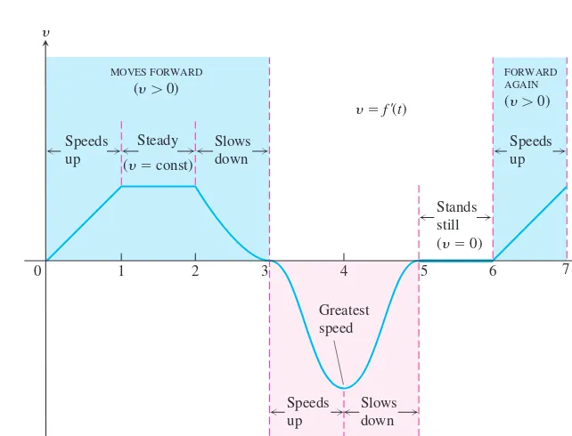
particle moves forward for the first 3 sec, moves backward for the next 2 sec, stands still
for a second, and moves forward again. The particle achieves its greatest speed at time
while moving backward.
t
=
4 ,
y
=
ƒ
¿
std
DEFINITION
Speed
Speed
is the absolute value of velocity.
Speed
= ƒ
y
std
ƒ =
`
ds
dt
`
0 1 2 3 4 5 6 7
MOVES FORWARD
(y 0)
MOVES BACKWARD
(y 0)
FORWARD AGAIN
(y 0)
Speeds up
Speeds up
Speeds up
Slows down Slows
down Steady
(y const)
y f '(t)
Stands still (y 0)
t (sec)
Greatest speed
y
FIGURE 3.15 The velocity graph for Example 3.