Beginning
Apache Pig
Big Data Processing Made Easy
—
Beginning
Apache Pig
Big Data Processing Made Easy
Balaswamy Vaddeman
Hyderabad, Andhra Pradesh, India
ISBN-13 (pbk): 978-1-4842-2336-9 ISBN-13 (electronic): 978-1-4842-2337-6
DOI 10.1007/978-1-4842-2337-6
Library of Congress Control Number: 2016961514
Copyright © 2016 by Balaswamy Vaddeman
This work is subject to copyright. All rights are reserved by the Publisher, whether the whole or part of the material is concerned, specifically the rights of translation, reprinting, reuse of illustrations, recitation, broadcasting, reproduction on microfilms or in any other physical way, and transmission or information storage and retrieval, electronic adaptation, computer software, or by similar or dissimilar methodology now known or hereafter developed.
Trademarked names, logos, and images may appear in this book. Rather than use a trademark symbol with every occurrence of a trademarked name, logo, or image we use the names, logos, and images only in an editorial fashion and to the benefit of the trademark owner, with no intention of infringement of the trademark.
The use in this publication of trade names, trademarks, service marks, and similar terms, even if they are not identified as such, is not to be taken as an expression of opinion as to whether or not they are subject to proprietary rights.
While the advice and information in this book are believed to be true and accurate at the date of publication, neither the authors nor the editors nor the publisher can accept any legal responsibility for any errors or omissions that may be made. The publisher makes no warranty, express or implied, with respect to the material contained herein.
Managing Director: Welmoed Spahr Lead Editor: Celestin Suresh John Technical Reviewer: Manoj R. Patil
Editorial Board: Steve Anglin, Pramila Balan, Laura Berendson, Aaron Black, Louise Corrigan, Jonathan Gennick, Robert Hutchinson, Celestin Suresh John, Nikhil Karkal, James Markham, Susan McDermott, Matthew Moodie, Natalie Pao, Gwenan Spearing
Distributed to the book trade worldwide by Springer Science+Business Media New York, 233 Spring Street, 6th Floor, New York, NY 10013. Phone 1-800-SPRINGER, fax (201) 348-4505, e-mail [email protected], or visit www.springeronline.com. Apress Media, LLC is a California LLC and the sole member (owner) is Springer Science + Business Media Finance Inc (SSBM Finance Inc). SSBM Finance Inc is a Delaware corporation.
For information on translations, please e-mail [email protected], or visit www.apress.com. Apress and friends of ED books may be purchased in bulk for academic, corporate, or promotional use. eBook versions and licenses are also available for most titles. For more information, reference our Special Bulk Sales–eBook Licensing web page at www.apress.com/bulk-sales.
Any source code or other supplementary materials referenced by the author in this text are available to readers at www.apress.com. For detailed information about how to locate your book’s source code, go to www.apress.com/source-code/. Readers can also access source code at SpringerLink in the Supplementary Material section for each chapter.
The late Kammari Rangaswamy (Teacher)
The late Niranjanamma (Mother)
v
Contents at a Glance
About the Author ... xix
About the Technical Reviewer ... xxi
Acknowledgments ... xxiii
■
Chapter 1: MapReduce and Its Abstractions ... 1
■
Chapter 2: Data Types ... 21
■
Chapter 3: Grunt ... 33
■
Chapter 4: Pig Latin Fundamentals ... 41
■
Chapter 5: Joins and Functions ... 69
■
Chapter 6: Creating and Scheduling Workflows Using
Apache Oozie ... 89
■
Chapter 7: HCatalog ... 103
■
Chapter 8: Pig Latin in Hue ... 115
■
Chapter 9: Pig Latin Scripts in Apache Falcon ... 123
■
Chapter 10: Macros ... 137
■
Chapter 11: User-Defined Functions ... 147
■
Chapter 12: Writing Eval Functions ... 157
■
Chapter 13: Writing Load and Store Functions ... 171
■
Chapter 14: Troubleshooting ... 187
vi
■
Chapter 16: Optimization ... 209
■
Chapter 17: Hadoop Ecosystem Tools ... 225
■
Appendix A: Built-in Functions ... 249
■
Appendix B: Apache Pig in Apache Ambari ... 257
■
Appendix C: HBaseStorage and ORCStorage Options ... 261
vii
Contents
About the Author ... xix
About the Technical Reviewer ... xxi
Acknowledgments ... xxiii
■
Chapter 1: MapReduce and Its Abstractions ... 1
Small Data Processing ... 1
Relational Database Management Systems ... 3
Data Warehouse Systems ... 3
Parallel Computing ... 4
GFS and MapReduce ... 4
Apache Hadoop ... 4
Problems with MapReduce ... 13
Cascading ... 13
Apache Hive ... 15
Apache Pig ... 16
Summary ... 20
■
Chapter 2: Data Types ... 21
Simple Data Types ... 22
int ... 22
long ... 22
float ... 22
double ... 23
viii
boolean ... 23
bytearray ... 23
datetime ... 23
biginteger ... 24
bigdecimal ... 24
Summary of Simple Data Types ... 24
Complex Data Types ... 24
map... 25
tuple... 26
bag ... 26
Summary of Complex Data Types ... 27
Schema ... 28
Casting ... 28
Casting Error ... 29
Comparison Operators ... 29
Identifiers ... 30
Boolean Operators ... 31
Summary ... 31
■
Chapter 3: Grunt ... 33
Invoking the Grunt Shell ... 33
Commands ... 34
The fs Command ... 34
The sh Command ... 35
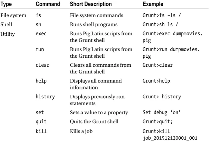
Utility Commands ... 36
help ... 36
history ... 36
quit ... 36
ix
set ... 37
clear ... 38
exec ... 38
run ... 39
Summary of Commands ... 39
Auto-completion ... 40
Summary ... 40
■
Chapter 4: Pig Latin Fundamentals ... 41
Running Pig Latin Code ... 41
Grunt Shell ... 41
Pig -e ... 42
Pig -f ... 42
Embed Pig Code in a Java Program ... 42
Hue ... 44
Pig Operators and Commands ... 44
Load ... 45
store ... 47
dump ... 48
version ... 48
Foreach Generate ... 48
filter ... 50
Limit ... 51
Assert ... 51
SPLIT ... 52
SAMPLE ... 53
FLATTEN ... 53
import ... 54
define ... 54
x
RANK ... 55
Union ... 56
ORDER BY ... 57
GROUP ... 59
Stream ... 61
MAPREDUCE ... 62
CUBE ... 63
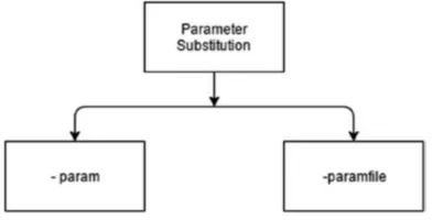
Parameter Substitution ... 65
-param ... 65
-paramfile ... 66
Summary ... 67
■
Chapter 5: Joins and Functions ... 69
Join Operators ... 70
Equi Joins ... 70
cogroup ... 72
CROSS ... 73
Functions ... 74
String Functions ... 74
Mathematical Functions ... 76
Date Functions ... 78
EVAL Functions ... 80
Complex Data Type Functions ... 81
Load/Store Functions ... 82
Summary ... 87
■
Chapter 6: Creating and Scheduling Workflows Using
Apache Oozie ... 89
Types of Oozie Jobs ... 89
Using a Pig Latin Script as Part of a Workflow ... 91
Writing job.properties ... 91
workflow.xml ... 91
Uploading Files to HDFS ... 93
Submit the Oozie Workflow ... 93
Scheduling a Pig Script ... 94
Writing the job.properties File ... 94
Writing coordinator.xml ... 94
Upload Files to HDFS ... 96
Submitting Coordinator... 96
Bundle ... 96
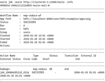
oozie pig Command ... 96
Command-Line Interface ... 98
Job Submitting, Running, and Suspending ... 98
Killing Job ... 98
Retrieving Logs ... 98
Information About a Job ... 98
Oozie User Interface ... 99
Developing Oozie Applications Using Hue ... 100
Summary ... 100
■
Chapter 7: HCatalog ... 103
Features of HCatalog ... 103
Command-Line Interface ... 104
show Command ... 105
Data Definition Language Commands ... 105
WebHCatalog ... 107
Executing Pig Latin Code ... 108
Running a Pig Latin Script from a File ... 108
HCatLoader Example ... 109
Writing the Job Status to a Directory ... 109
HCatLoader and HCatStorer ... 110
Reading Data from HCatalog ... 110
Writing Data to HCatalog ... 110
Running Code ... 111
Data Type Mapping ... 112
Summary ... 113
■
Chapter 8: Pig Latin in Hue ... 115
Pig Module ... 115
My Scripts ... 116
Pig Helper ... 117
Auto-suggestion ... 117
UDF Usage in Script ... 118
Query History ... 118
File Browser ... 119
Job Browser ... 121
Summary ... 122
■
Chapter 9: Pig Latin Scripts in Apache Falcon ... 123
cluster ... 124
Interfaces ... 124
Locations ... 125
feed ... 126
Feed Types ... 126
Late Arrival... 127
Cluster ... 127
process ... 128
cluster ... 128
Failures ... 128
feed... 129
workflow ... 129
CLI ... 129
entity ... 129
Web Interface ... 130
Search ... 131
Create an Entity ... 131
Notifications ... 131
Mirror ... 131
Data Replication Using the Falcon Web UI... 131
Create Cluster Entities ... 132
Create Mirror Job ... 132
Pig Scripts in Apache Falcon ... 134
Oozie Workflow ... 134
Pig Script ... 135
Summary ... 136
■
Chapter 10: Macros ... 137
Structure ... 137
Macro Use Case ... 138
Macro Types ... 138
Internal Macro ... 139
dryrun ... 141
Macro Chaining ... 141
Macro Rules ... 142
Define Before Usage ... 142
Valid Macro Chaining ... 143
No Macro Within Nested Block ... 143
No Grunt Shell Commands ... 143
Invisible Relations... 143
Macro Examples ... 144
Macro Without Input Parameters Is Possible ... 144
Macro Without Returning Anything Is Possible ... 144
Summary ... 145
■
Chapter 11: User-Defined Functions ... 147
User-Defined Functions ... 148
Java ... 148
JavaScript ... 150
Other Languages ... 152
Other Libraries ... 154
PiggyBank ... 154
Apache DataFu ... 155
Summary ... 155
■
Chapter 12: Writing Eval Functions ... 157
MapReduce and Pig Features ... 157
Accessing the Distributed Cache ... 157
Accessing Counters ... 158
Reporting Progress ... 159
Output Schema and Input Schema in UDF ... 159
Other EVAL Functions ... 162
Algebraic... 162
Accumulator ... 168
Filter Functions ... 168
Summary ... 169
■
Chapter 13: Writing Load and Store Functions ... 171
Writing a Load Function ... 171
Loading Metadata ... 174
Improving Loader Performance ... 176
Converting from bytearray ... 176
Pushing Down the Predicate ... 177
Writing a Store Function ... 178
Writing Metadata ... 182
Distributed Cache ... 183
Handling Bad Records ... 184
Accessing the Configuration ... 185
Monitoring the UDF Runtime ... 185
Summary ... 186
■
Chapter 14: Troubleshooting ... 187
Illustrate ... 187
describe... 188
Dump ... 188
Explain ... 188
Plan Types ... 189
Modes ... 193
Unit Testing ... 195
Counters ... 198
Summary ... 199
■
Chapter 15: Data Formats ... 201
Compression ... 201
Sequence File ... 202
Parquet ... 203
Parquet File Processing Using Apache Pig ... 204
ORC... 205
Index ... 207
ACID ... 207
Predicate Pushdown ... 207
Data Types ... 207
Benefits ... 208
Summary ... 208
■
Chapter 16: Optimization ... 209
Advanced Joins ... 209
Small Files ... 209
User-Defined Join Using the Distributed Cache ... 210
Big Keys ... 212
Sorted Data ... 212
Best Practices ... 213
Choose Your Required Fields Early ... 213
Define the Appropriate Schema ... 213
Filter Data ... 214
Store Reusable Data ... 214
Use the Algebraic Interface ... 214
Use the Accumulator Interface ... 215
Combine Small Inputs ... 215
Prefer a Two-Way Join over Multiway Joins ... 216
Better Execution Engine ... 216
Parallelism... 216
Job Statistics ... 217
Rules ... 218
Partition Filter Optimizer ... 218
Merge foreach ... 218
Constant Calculator ... 219
Cluster Optimization ... 219
Disk Space ... 219
Separate Setup for Zookeeper ... 220
Scheduler ... 220
Name Node Heap Size ... 220
Other Memory Settings ... 221
Summary ... 222
■
Chapter 17: Hadoop Ecosystem Tools ... 225
Apache Zookeeper ... 225
Terminology ... 225
Applications ... 226
Command-Line Interface ... 227
Four-Letter Commands ... 229
Measuring Time ... 230
Cascading ... 230
Defining a Source ... 230
Defining a Sink ... 232
Pipes ... 233
Apache Spark ... 237
Core ... 238
SQL ... 240
Apache Tez ... 245
Presto ... 245
Architecture ... 246
Connectors ... 247
Pushdown Operations ... 247
Summary ... 247
■
Appendix A: Built-in Functions ... 249
■
Appendix B: Apache Pig in Apache Ambari ... 257
Modifying Properties ... 258
Service Check ... 258
Installing Pig ... 259
Pig Status ... 259
Check All Available Services ... 259
Summary ... 260
■
Appendix C: HBaseStorage and ORCStorage Options ... 261
HBaseStorage ... 261
Row-Based Conditions ... 261
Timestamp-Based Conditions ... 262
Other Conditions ... 262
OrcStorage ... 263
About the Author
Balaswamy Vaddeman is a thinker, blogger, and serious and self-motivated big data evangelist with 10 years of experience in IT and 5 years of experience in the big data space. His big data experience covers multiple areas such as analytical applications, product development, consulting, training, book reviews, hackathons, and mentoring. He has proven himself while delivering analytical applications in the retail, banking, and finance domains in three aspects (development, administration, and architecture) of Hadoop-related technologies. At a startup company, he developed a Hadoop-based product that was used for delivering analytical applications without writing code.
About the Technical
Reviewer
Manoj R. Patil is a big data architect at TatvaSoft, an IT services and consulting firm. He has a bachelor’s of engineering degree from COEP in Pune, India. He is a proven and highly skilled business intelligence professional with 17 years of information technology experience. He is a seasoned BI and big data consultant with exposure to all the leading platforms such as Java EE, .NET, LAMP, and so on. In addition to authoring a book on Pentaho and big data, he believes in knowledge sharing, keeps himself busy in corporate training, and is a passionate teacher. He can be reached at on Twitter @manojrpatil and at https:// in.linkedin.com/in/manojrpatil on LinkedIn.
Acknowledgments
Writing a book requires a great team. Fortunately, I had a great team for my first project. I am deeply indebted to them for making this project reality.
I would like to thank the publisher, Apress, for providing this opportunity. Special thanks to Celestin Suresh John for building confidence in me in the initial stages of this project.
Special thanks to Subha Srikant for your valuable feedback. This project would have not been in this shape without you. In fact, I have learned many things from you that could be useful for my future projects also.
Thank you, Manoj R. Patil, for providing valuable technical feedback. Your contribution added a lot of value to this project.
Thank you, Dinesh Kumar, for your valuable time.
MapReduce and Its
Abstractions
In this chapter, you will learn about the technologies that existed before Apache Hadoop, about how Hadoop has addressed the limitations of those technologies, and about the new developments since Hadoop was released.
Data consists of facts collected for analysis. Every business collects data to understand their business and to take action accordingly. In fact, businesses will fall behind their competition if they do not act upon data in a timely manner. Because the number of applications, devices, and users is increasing, data is growing exponentially. Terabytes and petabytes of data have become the norm. Therefore, you need better data management tools for this large amount of data.
Data can be classified into these three types:
• Small data: Data is considered small data if it can be measured in gigabytes. • Big data: Big data is characterized by volume, velocity, and variety.
Volume refers to the size of data, such as terabytes and more. Velocity refers to the age of data, such as real-time, near-real-time, and streaming data. Variety talks about types of data; there are mainly three types of data: structured, semistructured, and unstructured.
• Fast data: Fast data is a type of big data that is useful for the real-time
presentation of data. Because of the huge demand for real-time or near-real-time data, fast data is evolving in a separate and unique space.
Small Data Processing
Many tools and technologies are available for processing small data. You can use languages such as Python, Perl, and Java, and you can use relational database management systems (RDBMSs) such as Oracle, MySQL, and Postgres. You can even use data warehousing tools and extract/transform/load (ETL) tools. In this section, I will discuss how small data processing is done.
Electronic supplementary material The online version of this chapter
Assume you have the following text in a file called fruits: Apple, grape
Apple, grape, pear Apple, orange
Let’s write a program in a shell script that first filters out the word pear and then counts the number of words in the file. Here’s the code:
cat fruits|tr ',' '\n'|grep -v -i 'pear'|sort -f|uniq -c –i This code is explained in the following paragraphs.
In this code, tr (for “translate” or “transliterate”) is a Unix program that takes two inputs and replaces the first set of characters with the second set of characters. In the previous program, the tr program replaces each comma (,) with a new line character (\n). grep is a command used for searching for specific text. So, the previous program performs an inverse search on the word pear using the -v option and ignores the case using -i.
The sort command produces data in sorted order. The -f option ignores case while sorting.
uniq is a Unix program that combines adjacent lines from the input file for reporting purposes. In the previous program, uniq takes sorted words from the sort command output and generates the word count. The -c option is for the count, and the -i option is for ignoring case.
The program produces the following output: Apple 3
Grape 2 Orange 1
You can divide program functionality into two stages; first is tokenize and filtering, and second is aggregation. Sort is supporting functionality of aggregation. Figure 1-1 shows the program flow.
Figure 1-1. Program flow
Relational Database Management Systems
RDBMSs were developed based on the relational model founded by E. F. Codd. There are many commercial RDBMS products such as Oracle, SQL Server, and DB2. Many open source RDBMSs such as MySQL, Postgres, and SQLite are also popular. RDBMSs store data in tables, and you can define relations between tables.
Here are some advantages of RDBMSs:
• RDBMS products come with sophisticated query languages
that can easily retrieve data from multiple tables with multiple conditions.
• The query language used in RDBMSs is called Structured Query
Language (SQL); it provides easy data definition, manipulation, and control.
• RDBMSs also support transactions.
• RDBMSs support low-latency queries so users can access
databases interactively, and they are also useful for online transaction processing (OLTP).
RDBMSs have these disadvantages:
• As data is stored in table format, RDBMSs support only
structured data.
• You need to define a schema at the time of loading data. • RDBMSs can scale only to gigabytes of data, and they are mainly
designed for frequent updates.
Because the data size in today’s organizations has grown exponentially, RDBMSs have not been able to scale with respect to data size. Processing terabytes of data can take days.
Having terabytes of data has become the norm for almost all businesses. And new data types like semistructured and unstructured have arrived. Semistructured data has a partial structure like in web server log files, and it needs to be parsed like Extensible Markup Language (XML) in order to analyze it. Unstructured data does not have any structure; this includes images, videos, and e-books.
Data Warehouse Systems
Data warehouse systems were introduced to address the problems of RDBMSs. Data warehouse systems such as Teradata are able to scale up to terabytes of data, and they are mainly used for OLAP use cases.
Data warehousing systems have these disadvantages:
• Data warehouse systems are a costly solution.
• They still cannot process other data types such as semistructured
and unstructured data.
All traditional data-processing technologies experience a couple of common problems: storage and performance.
Computing infrastructure can face the problem of node failures. Data needs to be available irrespective of node failures, and storage systems should be able to store large volumes of data.
Traditional data processing technologies used a scale-up approach to process a large volume of data. A scale-up approach adds more computing power to existing nodes, so it cannot scale to petabytes and more because the rest of computing infrastructure becomes a performance bottleneck.
Growing storage and processing needs have created a need for new technologies such as parallel computing technologies.
Parallel Computing
The following are several parallel computing technologies.
GFS and MapReduce
Google has created two parallel computing technologies to address the storage and processing problems of big data. They are Google File System (GFS) and MapReduce. GFS is a distributed file system that provides fault tolerance and high performance on commodity hardware. GFS follows a master-slave architecture. The master is called Master, and the slave is called ChunkServer in GFS. MapReduce is an algorithm based on key-value pairs used for processing a huge amount of data on commodity hardware. These are two successful parallel computing technologies that address the storage and processing limitations of big data.
Apache Hadoop
Apache Hadoop is an open source framework used for storing and processing large data sets on commodity hardware in a fault-tolerant manner.
Hadoop was written by Doug Cutting and Mark Cafarella in 2006 while working for Yahoo to improve the performance of the Nutch search engine. Cutting named it after his son’s stuffed elephant toy. In 2007, it was given to the Apache Software Foundation.
Initially Hadoop was adopted by Yahoo and, later, by companies like Facebook and Microsoft. Yahoo has about 100,000 CPUs and 40,000 nodes for Hadoop. The largest Hadoop cluster has about 4,500 nodes. Yahoo runs about 850,000 Hadoop jobs every day. Unlike conventional parallel computing technologies, Hadoop follows a scale-out strategy, which makes it more scalable. In fact, Apache Hadoop had set a benchmark by sorting 1.42 terabytes per minute.
Moore’s law says the processing capability of a machine will double every two years. Kryder’s law says the storage capacity of disks will grow faster than Moore’s law. The cost of computing and storage devices will go down every day, and these two factors can support more scalable technologies. Apache Hadoop was designed while keeping these things in mind, and parallel computing technologies like this will become more common going forward.
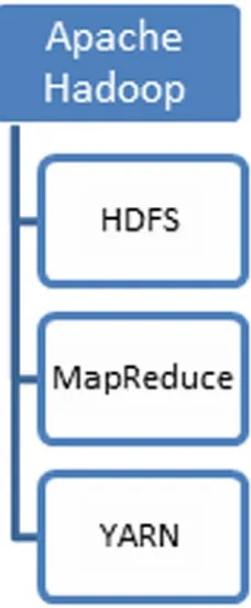
The latest Apache Hadoop contains three modules, as shown in Figure 1-2. They are HDFS, MapReduce, and Yet Another Resource Negotiator (YARN).
Figure 1-2. The three components of Hadroop
HDFS
Assume you have a replication factor of 3, a block size of 64 MB, and 640 MB of data needs to be uploaded into HDFS. At the time of uploading the data into HDFS, 640 MB is divided into 10 blocks with respect to block size. Every block is stored on three nodes, which would consume 1920 MB of space on a cluster.
HDFS follows a master-slave architecture. The master is called the name node, and the slave is called a data node. The data node is fault tolerant because the same block is replicated to two more nodes. The name node was a single point of failure in initial versions; in fact, Hadoop used to go down if the name node crashed. But Hadoop 2.0+ versions have high availability of the name node. If the active name node is down, the standby name node becomes active without affecting the running jobs.
MapReduce
MapReduce is key-value programming model used for processing large data sets. It has two core functions: Map and Reduce. They are derived from functional programming languages. Both functions take a key-value pair as input and generate a key-value pair as output.
The Map task is responsible for filtering operations and preparing the data required for the Reduce tasks. The Map task will generate intermediate output and write it to the hard disk. For every key that is being generated by the Map task, a Reduce node is identified and will be sent to the key for further processing.
The Map task takes the key-value pair as input and generates the key-value pair as output.
(key1, value1) ---> Map Task---> (Key2, Valu2)
The Reduce task is responsible for data aggregation operations such as count, max, min, average, and so on. A reduce operation will be performed on a per-key basis. Every functionality can be expressed in MapReduce.
The Reduce task takes the key and list of values as input and generates the key and value as output.
(key2, List (value2))---> Reduce Task ---> (Key3, value3)
In addition to the Map and Reduce tasks, there is an extra stage called the combiner to improve the performance of MapReduce. The combiner will do partial aggregation on the Map side so that the Map stage has to write less data to disk.
Source and Sink are HDFS directories. When you upload data to HDFS, data is divided into chunks called blocks. Blocks will be processed in a parallel manner on all available nodes.
The first stage is Map, which performs filtering and data preparation after tokenization. All Map tasks (M1, M2, and M3) will do the initial numbering for words that are useful for the final aggregation. And M2 filters out the word pear.
The key and list of its values are retrieved from the Map output and sent to the reducer node. For example, the Apple key and its values (1, 1, 1) are sent to the reducer node R1. The reducer aggregates all values to generate the count output.
Between Map and Reduce, there is an internal stage called shuffling where the reducer node for the map output is identified.
You will now see how to write the same word count program using MapReduce. You first need to write a mapper class for the Map stage.
Writing a Map Class
The following is the Map program that is used for the same tokenization and data filtering as in the shell script discussed earlier:
import java.io.IOException; import java.util.StringTokenizer; import org.apache.hadoop.io.IntWritable; import org.apache.hadoop.io.LongWritable; import org.apache.hadoop.io.Text;
import org.apache.hadoop.mapreduce.Mapper;
public class FilterMapper extends Mapper<LongWritable, Text, Text, IntWritable> { private final static IntWritable one = new IntWritable(1);
private Text word = new Text();
public void map(LongWritable offset, Text line, Context context) throws IOException, InterruptedException {
//tokenize line with comma as delimiter
StringTokenizer itr = new StringTokenizer(line.toString(),","); //Iterate all tokens and filter pear word
String strToken=itr.nextToken(); if(!strToken.equals("pear")){
//converting string data type to text data type of mapreduce word.set(strToken);
context.write(word, one);//Map output }
} } }
The Map class should extend the Mapper class, which has parameters for the input key, input value, output key, and output value. You need to override the map() method. This code specifies LongWritable for the input key, Text for the input value, Text for the output key, and IntWritable for the output value.
In the map() method, you use StringTokenizer to convert a sentence into words. You are iterating words using a while loop, and you are filtering the word pear using an if loop. The Map stage output is written to context.
For every run of the map() method, the line offset value is the input key, the line is the input value, the word in the line will become an output key, and 1 is the output value, as shown in Figure 1-4.
Figure 1-4. M2 stage
Figure 1-5. Map output without the combiner
The map() method runs once per every line. It tokenizes the line into words, and it filters the word pear before writing other words with the default of 1.
If the combiner is available, the combiner is run before the Reduce stage. Every Map task will have a combiner task that will produce aggregated output. Assume you have two apple words in the second line that is processed by the M2 map task.
9
Even combiner follows the key-value paradigm. Like the Map and Reduce stages, it will have an input key and input value and also an output key and output value. The combiner will write its output data to disk after aggregating the map output data. The combiner will write relatively less data to disk as it is aggregated, and less data is shuffled to the Reduce stage. Both these things will improve the performance of MapReduce.Figure 1-6 shows the combiner writing aggregated data that is apple,2 here.
Figure 1-6. The combiner writing aggregated data
Writing a Reduce Class
The following is a reducer program that does the word count on the map output and runs after the Map stage if the combiner is not available:
import java.io.IOException;
import org.apache.hadoop.io.IntWritable; import org.apache.hadoop.io.Text;
import org.apache.hadoop.mapreduce.Reducer;
public class WordCountReducer extends Reducer<Text, IntWritable, Text, IntWritable> {
private IntWritable count = new IntWritable();
public void reduce(Text word, Iterable<IntWritable> values, Context context) throws IOException, InterruptedException {
int sum = 0;
// add all values for a key i.e. word for (IntWritable val : values) { sum += val.get();
}
count.set(sum);//type cast from int to IntWritable context.write(word, count);
} }
For every run of reducer, the Map output key and its list of values are passed to the reduce() method as input. The list of values is iterated using a for loop because they are already iterable. Using the get() method of IntWritable, you get the value of the Java int data type that you would add to the sum variable. After completing the reduce() method for the partial word key, the word and count are generated as the reducer output. The reduce() method is run once per key, and the Reduce stage output is written to context just like map output. Figure 1-7 shows apple and the list of values (1,1,1) processed by Reduce task R2.
Figure 1-7. Reduce task R2
Writing a main Class
The following is the main class that generates the word count using the mapper class and the reducer class:
import org.apache.hadoop.conf.Configuration; import org.apache.hadoop.fs.Path;
import org.apache.hadoop.io.IntWritable; import org.apache.hadoop.io.Text; import org.apache.hadoop.mapreduce.Job;
import org.apache.hadoop.mapreduce.lib.input.FileInputFormat; import org.apache.hadoop.mapreduce.lib.output.FileOutputFormat; public class WordCount {
public static void main(String[] args) throws Exception { Configuration conf = new Configuration();
Job job = Job.getInstance(conf, "word count"); job.setJarByClass(WordCount.class);
job.setMapperClass(FilterMapper.class); job.setReducerClass(WordCountReducer.class); job.setOutputKeyClass(Text.class);
job.setOutputValueClass(IntWritable.class); //take input path from command line
FileInputFormat.addInputPath(job, new Path(args[0])); //take output path from command line
FileOutputFormat.setOutputPath(job, new Path(args[1])); System.exit(job.waitForCompletion(true) ? 0 : 1); }
}
You first pass the main class name in setJarByClass so that the framework will start executing from that class. You set the mapper class and the reducer class on the job object using the setMapperClass and setReducerClass methods.
FileInputFormat says the input format is available as a normal file. And you are passing the job object and input path to it. FileOutputFormat says the output format is available as a normal file. And you are passing the job object and output path to it. FileInputFormat and FileOutputFormat are generic classes and will handle any file type, including text, image, XML, and so on. You need to use different classes for handling different data formats. TextInputFormat and TextOutputFormat will handle only text data. If you want to handle binary format data, you need to use Sequencefileinputformat and sequencefileoutputformat.
If you want to specify key and value data types, you can control them from this program for both the mapper and the reducer.
Running a MapReduce Program
You need to create a .jar file with the previous three programs. You can generate a .jar file using the Eclipse export option. If you are creating a .jar file on other platforms like Windows, you need to transfer this .jar file to one of the nodes in the Hadoop cluster using FTP software such as FileZilla or WinScp. Once the JAR is available on the Hadoop cluster, you can use the Hadoop jar command to run the MapReduce program, like so: Hadoop jar /path/to/wordcount.jar Mainclass InputDir OutputDir
Most grid computing technologies send data to code for processing. Hadoop works in the opposite way; it sends code to data. Once the previous command is submitted, the Java code is sent to all data nodes, and they will start processing data in a parallel manner. The final output is written to files in the output directory, and by default the job will fail if the output directory already exists. The total number of files will depend on the number of reducers.
1. Prepare data that is suitable for the combiner and write a program for word count using MapReduce that includes the combiner stage.
YARN
In earlier Hadoop versions, MapReduce was responsible for data processing, resource management, and scheduling. In Hadoop 2.0, resource management and scheduling have been separated from MapReduce to create a new service called YARN. With YARN, several applications such as in-memory computing systems and graph applications can co-exist with MapReduce.
application master is, in effect, a framework-specific library and is tasked with negotiating resources from the resource manager and working with the node manager to execute and monitor the tasks.
Benefits
Now that you know about the three components that make up Apache Hadoop, here are the benefits of Hadoop:
• Because Apache Hadoop is an open source software framework, it
is a cost-effective solution for processing big data. It also runs on commodity hardware.
• Hadoop does not impose a schema on load; it requires a schema
only while reading. So, it can process all types of data, that is, structured, semistructured, and unstructured data.
• Hadoop is scalable to thousands of machines and can process
data the size of petabytes and beyond.
• Node failures are normal in a big cluster, and Hadoop is fault
tolerant. It can reschedule failed computations.
• Apache Hadoop is smart parallel computing framework that
sends code to data rather than data to code. This code-to-data approach consumes fewer network resources.
Use Cases
Initially Hadoop was developed as a batch-processing framework, but after YARN, Hadoop started supporting all types of applications such as in-memory and graph applications.
• Yahoo uses Hadoop in web searches and advertising areas. • Twitter has been using Hadoop for log analysis and tweet analysis. • Hadoop had been used widely for image processing and video
analytics.
• Many financial companies are using Hadoop for churn analysis,
fraud detection, and trend analytics.
• Many predictive analytics have been done using Hadoop in the
healthcare industry.
• LinkedIn’s “People You May Know” feature is implemented by
Problems with MapReduce
MapReduce is a low-level API. You need to think in terms of the key and value every time you use it. In addition, MapReduce has a lengthy development time. It cannot be used for ad hoc purposes. You need MapReduce abstractions, which hide the key-value programming paradigm from the user.
Chris Wensel addressed this problem by creating the Java-based MapReduce abstraction called Cascading.
Cascading
Cascading is a Java-based MapReduce abstraction used for building big data applications. It hides the key-value complexity of MapReduce from the programmer so that the programmer can focus on the business logic, unlike MapReduce. Cascading also has an API that provides several built-in analytics functions. You do not need to write functions such as count, max, and average, unlike MapReduce. It also provides an API for integration and scheduling apart from processing.
Cascading is based on a metaphor called pipes and filters. Basically, Cascading allows you to define a pipeline that contains a list of pipes. Once the pipe output is passed as an input to another pipeline, the pipelines will merge, join, group, and split the data apart from performing other operations on data. The pipeline will read data from the source tap and will write to the sink tap. The source tap, sink tap, and their pipeline are defined as a flow in Cascading. Figure 1-8 shows a sample flow of Cascading.
Figure 1-8. Sample flow of Cascading
Here is how to write a word count program in Cascading: import java.util.Properties;
import cascading.flow.Flow;
import cascading.flow.local.LocalFlowConnector; import cascading.operation.aggregator.Count;
import cascading.pipe.Every;
public static void main(String[] args) {
Tap srcTap = new FileTap( new TextLine( new Fields(new String[]{"line"})) , args[0] );
Tap sinkTap = new FileTap( new TextLine( new Fields(new String[]{"word" , "count"})), args[1], SinkMode.REPLACE );
Pipe words=new Each("start",new RegexSplitGenerator(",")); Pipe group=new GroupBy(words);
Count count=new Count();
Pipe wcount=new Every(group, count); Properties properties = new Properties();
AppProps.setApplicationJarClass( properties, WordCount.class ); LocalFlowConnector flowConnector = new LocalFlowConnector();
Flow flow = flowConnector.connect( "wordcount", srcTap, sinkTap, wcount ); flow.complete();
} }
In this code, the Fields class is used for defining column names. TextLine will hold field names and also data path details. srcTap will have source field names and input path. snkTap will define output field names and the output path. FileTap is used to read data from the local file system. You can use HFS to run it on the HDFS data. SinkMode. REPLACE will replace the output data if it already exists in the output directory specified.
Each operator is allowed to perform an operation on each line. Here you are using the RegexSplitGenerator function that splits every line of text into words using a comma (,) as the delimiter. You are defining this pipe as words.
The GroupBy class works on the words pipe to arrange words into groups and creates a new pipe called group. Later you will create a new pipe account that will apply the count operation on every group using the Every operator.
Properties allow you to provide values to properties. You are not setting any properties. You will use the put() method to insert property values.
properties.put("mapred.reduce.tasks", -1);
You will create an object for LocalFlowConnector and will define the flow
LocalFlowConnector will help you to create a local flow that can be run on the local file system. You can use HadoopFlowConnector for creating a flow that works on the Hadoop file system. flow.complete() will start executing the flow.
1. Modify the previous Cascading program to filter the word pear.
Benefits
These are the benefits of Cascading:
• Like MapReduce, it can process all types of data, such as
structured, semistructured, and unstructured data.
• Though it is a MapReduce abstraction, it is still easy to extend it. • You can rapidly build big data applications using Cascading. • Cascading is unit-testable.
• It follows fail-fast behavior, so it is easy to troubleshoot problems. • It is proven as an enterprise tool and can seamlessly integrate
with data-processing tools.
Use Cases
Cascading can be used as an ETL, batch-processing, machine-learning, and big data product development tool. Cascading can be used in many industries such as social media, healthcare, finance, and telecom.
Apache Hive
A traditional warehouse system is an expensive solution that will not scale to big data. Facebook has created a warehouse solution called Hive. Hive is built on top of Hadoop to simplify big data processing for business intelligence users and tools. The SQL interface in Hive has made it widely adopted both within Facebook and even outside of Facebook, especially after it was provided as open source to the Apache Software Foundation. It supports indexing and ACID properties.
Hive has some useful components such as the metastore, Hive Query Language, HCatalog, and Hive Server.
• The metastore stores table metadata and stats in an RDBMS such
as MySQL, Postgres, or Oracle. By default it stores metadata in the embedded RDBMS Apache Derby.
• The Hive Query Language (HQL) is a SQL interface to Hadoop
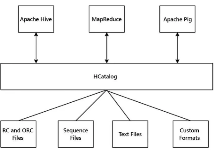
• HCatalog is table and storage management tool that enables big
data processing tools to easily read and write data.
• HiveServer2 is a Thrift client that enables BI tools to connect to
Hive and retrieve results.
Here is how to write a word count program in Apache Hive: select word,count(word) as count
from
(SELECT explode(split(sentence, ',')) AS word FROM texttable)temp group by word
This writes a Hive query that filters the word pear and generates the word count. split is used to tokenize sentences into words after applying a comma as a delimiter. explode is a table-generating function that converts every line of words into rows and names new column data as words. This creates a new temporary table called temp, generates a word-wise count using the group by and count functions from the temp table, and creates an alias called count. This query output is displayed on the console. You can create a new table from this table by prepending the create table as select statement like below.
Create table wordcount as
Benefits
Hive is a scalable data warehousing system. Building a Hive team is easy because of its SQL interface. Unlike MapReduce, it is suitable for ad hoc querying. With many BI tools available on top of Hive, people without much programming experience can get insights from big data. It can easily be extensible using user-defined functions (UDFs). You can easily optimize code and also support several data formats such as text, sequence, RC, and ORC.
Use Cases
Because Hive has a SQL interface, it was a quickly adopted Hadoop abstraction in businesses. Apache Hive is used in data mining, R&D, ETL, machine learning, and reporting areas. Many business intelligence tools provide facilities to connect to a Hive warehouse. Some tools include Teradata, Aster data, Tableau, and Cognos.
Apache Pig
It was developed by a team at Yahoo for researchers around 2006. In 2007, it was open sourced to the Apache Software Foundation. The purpose of Pig was to enable ad hoc querying on Apache Hadoop.
Here is how to write a word count program in Apache Pig: input = LOAD '/path/to/input/file/' AS (line:Chararray);
Words = FOREACH input GENERATE FLATTEN(TOKENIZE(line,',')) AS word; Grouped = GROUP words BY word;
wordcount = FOREACH Grouped GENERATE group, COUNT(word) as wordcount; store wordcount into '/path/to/output/dir';
The load operator reads the data from the specified path after applying the schema that is specified after the As word. Here line is the column name, and chararray is the data type. You are creating a relation called input.
The FOREACH processes line by line on the relation input, and generate applies the Tokenize and Flatten functions to convert sentences into plain words using a comma delimiter, and the column name is specified as word. These words are stored in a relation called words. Words are arranged into groups using the Group operator. The next line is applied on a relation called grouped that performs the count function on every group of words. You are defining the column name as wordcount. You will store the final output in another directory using the store operator. The dump operator can be used for printing the output on the console.
1. Change the previous program to filter the word pear.
Pig Latin code can be submitted using its CLI and even using the HUE user interface. Oozie can use Pig Latin code as part of its workflow, and Falcon can use it as part of feed management.
Pig vs. Other Tools
The Hadoop ecosystem has many MapReduce abstractions, as shown in Figure 1-9. You will learn how Apache Pig is compared against others.
Java Based
Data Warehouse
Scripting Platform
Cascading Apache Hive Apache Pig
MR Abstractions
MapReduce
MapReduce is a low-level API. Development efforts are required for even simple analytical functions. For example, joining data sets is difficult in MapReduce.
Maintainability and reuse of code are also difficult in MapReduce. Because of a lengthy development time, it is not suitable for ad hoc querying. MapReduce requires a learning curve because of its key-value programming complexity. Optimization requires many lines of code in MapReduce.
Apache Pig is easy to use and simple to learn. It requires less development time and is suitable for ad hoc querying. A simple word count in MapReduce might take around 60 lines of code. But Pig Latin can do it within five lines of code. You can easily optimize code in Apache Pig. Unlike MapReduce, you just need to specify two relations and their keys for joining two data sets.
Cascading
Cascading extensions are available in different languages. Scalding is Scala-based, Cascalog is Clojure-based, and PyCascading is Python-based. All are programming language–based. Though it takes relatively less development time than MapReduce, it cannot be used for ad hoc querying. In Pig Latin, the programming language is required only for advanced analytics, not for simple functions. The word count program in Cascading requires 30 lines of code, and Pig requires only five lines of code. Cascading’s pipeline will look similar to the data flow conceptually.
Apache Hive
Apache Hive was written only for a warehouse use case that can process only structured data that is available within tables. And it is declarative language that talks about what to achieve rather than how to achieve. Complex business applications require several lines of code that might have several subqueries inside. These queries are difficult to understand and are difficult to troubleshoot in case of issues. Query execution in Hive is from the innermost query to the outermost query. In addition, it takes time to understand the functionality of the query.
Pig is procedural language. Pig Latin can process all types of data: structured, semistructured, and unstructured including nested data. One of the main features of Pig is debugging. A developer can easily debug Pig Latin programs. Pig has a framework called Penny that is useful for monitoring and debugging Pig Latin jobs. The data flow language Pig Latin is written in step-by-step manner that is natural and easy to understand.
Use Cases
Apache Pig can be used for every business case where Apache Hadoop is used. Here are some of them:
• Apache Pig is a widely used big data–processing technology. More
than 60 percent of Hadoop jobs are Pig jobs at Yahoo.
• Twitter extensively uses Pig for log analysis, sentiment analysis,
and mining of tweet data.
• PayPal uses Pig to analyze transaction data and fraud detection. • Analysis of web logs is also done by many companies using Pig.
Pig Philosophy
Apache Pig has four founding principles that define the philosophy of Pig. These principles help users get a helicopter view of the technology. These principles also help developers to write new functionality with a purpose.
Pigs Eat Anything
Pig can process all types of data such as structured, semistructured, and unstructured data. It can also read data from multiple source systems like Hive, HBase, Cassandra, and so on. It supports many data formats such as text, sequence, ORC, and Parquet.
Pigs Live Anywhere
Apache Pig is big data–processing tool that was first implemented on Apache Hadoop. It can even process local file system data.
Pigs Are Domestic Animals
Like other domestic animals, pigs are friendly animals, and Apache Pig is user friendly. Apache Pig is easy to use and simple to learn. If a schema not specified, it takes the default schema. It applies the default load and store functions if not specified and applies the default delimiter if not given by the user. You can easily integrate Java, Python, and JavaScript code into Pig.
Pigs Fly
Summary
Traditional RDBMSs and data warehouse systems cannot scale to the growing size and needs of data management, so Google introduced two parallel computing technologies, GFS and MapReduce, to address big data problems related to storage and data
processing.
Doug Cutting, inspired by the Google technologies, created a technology called Hadoop with two modules: HDFS and MapReduce. HDFS and MapReduce are the same as Google GFS and MapReduce with respect to functionality. MapReduce has proven itself in big data processing and has become the base platform for current and future big data technologies.
As MapReduce is low level and not developer friendly, many abstractions were created to address different needs. Cascading is a Java-based abstraction that hides the key and value from the end user and allows you to develop big data applications. It is not suitable for ad hoc querying. Apache Hive is data warehouse for big data and supports only structured data; even a nontechnical person can generate reports using BI tools on top of Hive.
Data Types
In this chapter, you will start learning how to code using Pig Latin. This chapter covers data types, type casting among data types, identifiers, and finally some operators.
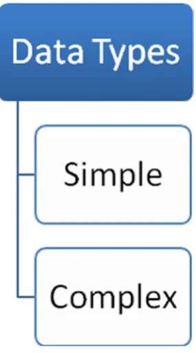
Apache Pig provides two data types. They are simple and complex, as specified in Figure 2-1. The simple data types include int, long, float, double, boolean, chararray, bytearray, datetime, biginteger, and bigdecimal. The complex data types are map, tuple, and bag.
In Pig Latin, data types are specified as part of the schema after the as keyword and within brackets. The field name is specified first and then the data type. A colon is used to separate the column name and data type.
Here is an example that shows how to use data types:
emp = load '/data/employees' as (eid:int,ename:chararray,gender:chararray);
Now you will learn all about the data types in both the simple and complex categories.
Simple Data Types
In this section, you will learn about the simple data types in detail with example code, including the size they support. Most of data types are derived from the Java language.
int
The int data type is a 4-byte signed integer similar to the integer in Java. It can contain values in the range of 2^31 to (2^31)–1, in other words, a minimum value of 2,147,483,648 and a maximum value of 2,147,483,647 (inclusive).
The following shows some sample code that uses the int data type:
Sales = load '/data/sales' as (eid:int);
long
The long data type is an 8-byte signed integer that is the same with respect to size and usage as in Java. It can contain values in the range of 2^63 to (2^63)–1. A lowercase l or an uppercase L is used to represent a long data type in Java. Similarly, you can use lowercase l or uppercase L as part of constant.
The following is an example that uses the long data type:
emp = load '/data/employees' as (DOB:long);
float
The float data type is a 4-byte floating-point number that is the same as float in Java. A lowercase f or an uppercase F is used to represent floats, for example, 34.2f or 34.2F.
The following is an example that uses the float data type:
double
double is an 8-byte floating-point number that is the same as double in Java. Unlike float or other data, no character is required to represent the double data type.
The following is an example that uses the double data type:
emp = load '/data/employees' as (salary:double);
chararray
The chararray data type is a character array in UTF-8 format. This data type is the same as string. You can use chararray when you are not sure of the type of data stored in a field. When you use an incorrect data type, Pig Latin returns a null value. It is a safe data type to use to avoid null values.
The following is an example that uses the chararray data type:
emp = load '/data/employees' as (country:chararray);
boolean
The boolean data type represents true or false values. This data type is case insensitive. Both True and tRuE are treated as similar in Boolean data.
The following is an example that uses the boolean data type.
emp = load '/data/employees' as (isWeekend:boolean);
bytearray
The bytearray data type is a default data type and stores data in BLOB format as a byte array. If you do not specify a data type, Pig Latin assigns the bytearray data type by default. Alternately, you can also specify the bytearray data type.
The following is an example that uses the bytearray data type:
emp = load '/data/employees' as (eid,ename,salary);
Here’s another example:
emp = load '/data/employees' as (eid:bytearray,ename:bytearray,salary:bytearray);
datetime
The following is an instance of this format: 2015-01-01T00:00:00.000+00:00.
emp = load '/data/employees' as (dateofjoining:datetime);
biginteger
The biginteger data type is the same as the biginteger in Java. If you have data bigger than long, then you use biginteger. The biginteger data type is particularly useful for representing credit card or debit card numbers.
Sales = load '/data/sales' as (cardnumber:biginteger);
bigdecimal
The bigdecimal data type is the same as bigdecimal in Java. The bigdecimal data type is used for data bigger than double. Here’s an example: 22.2222212145218886998.
Summary of Simple Data Types
Table 2-1 summarizes all the simple data types.Table 2-1. Simple Data Types
Type
Description
Example
int 4-byte 100
long 8-byte 100L or 100l
float 4-byte 100.1f or 100.1F
double 8-byte 100.1e2
biginteger Java biginteger 100000000000
bigdecimal Java bigdecimal 100.0000000001
boolean True/false true/false
chararray UTF-8 string Big data is everywhere
bytearray Binary data Binary data
datetime Date and time 2015:12:07T10:10:20.001+00.00
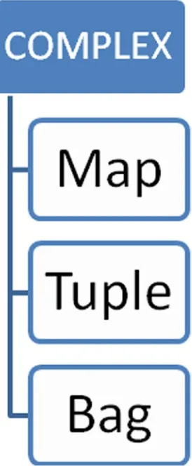
Complex Data Types
Figure 2-2. Complex data types
map
A map data type holds a set of key-value pairs. Maps are enclosed in straight brackets. The key and value are separated by the # character. The key should be the chararray data type and should be unique. While the value can hold any data type, the default is set to bytearray.
Here’s the syntax (the key-value pair needs to be present in a file):
[key1#value1,key2#value2,key3#value3,...]
Here’s an example:
[empname#Bala]
Here’s another example:
emp = load '/data/employees' as (M:map[chararray]);
The second example states the value of the data type is chararray.
If your data is not in the map data type format, you can convert the two existing fields into the map data type using the TOMAP function.
The following code converts the employee name and year of joining a company to the map data type:
emp = load 'employees' as (empname:chararray, year:int); empmap = foreach emp generate TOMAP(empname, year);
tuple
A tuple is an ordered set of fields and is enclosed in parentheses. A field can hold any data type including another tuple or bag. Fields are numbered beginning from 0. If field data is not available, then its value is set to a default of null.
For example, consider the following tuple:
(Bala,100,SSE)
This tuple has three data fields. Data in this example can be loaded using the following statement:
emp = load '/data/employees' as (T: tuple (empname:chararray, dno:int, desg:charray));
or the following statement:
emp = load '/data/employees' as (T: (empname:chararray, dno:int, desg:charray));
You can convert existing data fields into tuples with the TOTUPLE function. The following code converts fields with simple data types into tuples:
emp = load '/data/employees' as (ename:chararray, eid:int, desg:charray); emptuple=foreach emp generate TOTUPLE(ename, eid,desg);
bag
Here is the syntax for the bag data type:
{tuple1, tuple2, tuple3,...}
Here’s an example:
{(Bala, 1972, Software Engineer)}
Data for this example can be loaded using the following statement:
emp = load '/data/employees' as (B: bag {T: tuple (ename:chararray, empid:int, desg:charray)} );
or the following:
emp = load '/data/employees' as (B: {T: (ename:chararray, empid:int, desg:charray)});
There are two types of bags: outer bag and inner bag. Here is an example of data with an inner bag:
(1,{( Bala, 1972, Software Engineer)})
You can convert fields with simple data types into bag data types using the TOBAG function.
The following lines of code convert existing fields into bag data types.
emp = load '/data/employees' as (ename:chararray, empid:int, desg:charray); empbag=foreach emp generate TOBAG(ename,empid,desg);
Dump empbag;
({(Bala),(1972),(Software Engineer)})
Summary of Complex Data Types
Table 2-2 summarizes the complex data types.Table 2-2. Complex Data Types
Type
Description
Example
map Key and value [100#ApachePig]
tuple Set of fields (10,Pig)
Schema
Now you will look at how to check the available columns, and their data types, of a relation. To find out the schema of a relation, you can use the describe keyword.
The syntax for using describe is as follows:
Describe <<relation>>;
For example, the statement for describe usage is as follows:
emp = load '/data/emp' as (ename:chararray, eid:int, desg:chararray); Describe emp;
The output will read as follows:
emp: {ename:chararray, eid:int, desg:chararray}
You need not specify the data type in Pig Latin, as it assigns the default data type bytearray to all columns.
The following code specifies column names without data types:
Movies = load '/data/movies' as (moviename, year, genre); Describe Movies;
The output will read as follows:
Movies: {moviename:bytearray, year:bytearray, genre:bytearray}
Pig Latin allows you to load data without specifying a column name and data type. It uses the default numbering, starting from 0, and assigns the default data type. If you try to generate a schema for such a relation, Pig Latin will give the output Schema unknown. Whenever you perform operations on fields of such relations, Pig Latin will cast bytearray to the most suitable data type.
The following code does not specify column names and data types:
emp = load '/data/employees'; Describe emp;
emp: schema for emp unknown.
Casting
29
To perform casting from int to chararray, you can use the following code:empcode = foreach emp generate (chararray) empid;
bytearray is the most generic data type and can be cast to any data type. Casting
from bytearray to other data types occurs implicitly depending on the specified operation. To perform arithmetic operations, bytearray casting is performed to double. Similarly, casting from bytearray to datetime, chararray, and boolean data types occurs when the user performs the respective operations. bytearray can also be cast to the complex data types of map, tuple, and bag.
Casting Error
Both implicit casting and explicit casting throw an error if they cannot perform casting. For example, if you are performing a sum operation on two fields and one of them does not contain a numeric value, then implicit casting will throw an error.
If you are explicitly trying to cast from chararray to int and chararray does not have a numeric value, then explicit casting will throw an error.
Table 2-3 lists possible castings between different data types. For example, boolean can be cast to chararray but not to int because boolean is represented using true and false values, not 0 and 1.
Table 2-3. Possible Castings Between Different Data Types
From To
int
long
float
double
chararray
bytearray boolean
int NA Yes Yes Yes Yes No No
long Yes NA Yes Yes Yes No No
float Yes Yes NA Yes Yes NO No
double Yes Yes Yes NA Yes No No
chararray Yes Yes Yes Yes NA No Yes
bytearray Yes Yes Yes Yes Yes NA Yes
boolean No No No No Yes No NA
Comparison Operators
You can use the filter keyword to perform comparison operations. Here’s an example:
Year= filter emp by (year==1972);
You can also perform pattern matching as part of the filter keyword using the matches operator.
For instance, the following code searches for employees who have john in their names:
empjohn = filter emp by (ename matches ‘.*john*.’ ;
Identifiers
Identifiers may be names of fields, relations, aliases, variables, and so on. Identifiers always begin with an alphabet and can be followed by letters, numbers, and underscores.
Here are examples of correct names:
Moviename1_ Moviename5
Here are examples of incorrect names:
_movie $movie Movie$
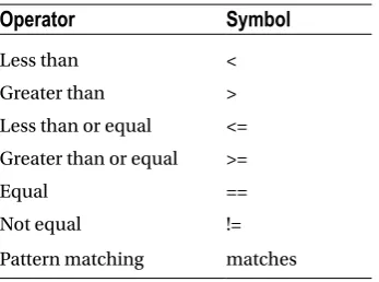
Table 2-4. Comparison Operations
Operator
Symbol
Less than <
Greater than >
Less than or equal <=
Greater than or equal >=
Equal ==
Not equal !=
Boolean Operators
Pig Latin includes Boolean operators such as AND, OR, NOT, and IN.
• AND returns true if all conditions are true.
• OR requires that at least one condition is true in order to return a
true value.
• NOT inverts the value, and IN represents a list of “or” conditions.
Boolean operators are specified in the filter statement.
The following code filters employees whose year of joining a company is either 1997 or 1980:
empyoj = FILTER emp BY (yearOJ==1997) OR (yearOJ==1980);
Summary
Grunt
In the previous chapter, you learned the Pig Latin fundamentals such as data types, type casting among data types, and operators. In this chapter, you will learn about the command-line interface (CLI) of Pig, called Grunt.
You can use Grunt for submitting Pig Latin scripts, controlling jobs, and accessing file systems, both local and HDFS, in Pig.
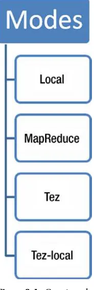
Invoking the Grunt Shell
You can start a Grunt shell in the following four modes: Local, MapReduce, Tez, and Tez-local.