Directory UMM :Data Elmu:jurnal:A:Agriculture, Ecosystems and Environment:Vol81.Issue1.Oct2000:

Uncertainties in the appraisal of water availability and

consequences for simulated sugarcane yield potentials

in São Paulo State, Brazil

M. van den Berg

a,∗

_{, P.A. Burrough}

b

_{, P.M. Driessen}

a

a_{Department of Environmental Sciences, Laboratory of Soil Science and Geology, Wageningen University,}

P.O. Box 37, 6700 AA Wageningen, The Netherlands

b_{Faculty of Geographical Sciences, Utrecht Centre for Environment and Landscape Dynamics (UCEL),}

Utrecht University; P.O. Box 80115, 3508 TC Utrecht, The Netherlands

Received 14 July 1999; received in revised form 5 January 2000; accepted 3 February 2000

Abstract

Summary crop growth models are promising tools for assessing crop yield potentials, but it is necessary to indicate un-certainties in model calculations that result from simplifying assumptions and errors/unun-certainties in model input data and parameter values. The present study attempts to do this for soil factors that affect the water balance of land-use systems with sugarcane (Saccharumspp. L.) on strongly weathered soils (mainly Ferralsols) in São Paulo State, Brazil. Propagation of

uncertainties were assessed for: (1) water retention characteristics of the soil; (2) effective rooting depth as limited by acid layers with large Al saturation (percentage of effective cation exchange capacity occupied by Al3+_{) and (3) possible errors}

originating from the methods used to calculate water withdrawal by roots. Probability density functions were constructed for the maximum effective rooting depth (RDM, cm), estimated on the basis of the soils’ Al saturation at 60–80 cm depth; and for ‘available’ water retained 2 days after field saturation (θ2d−1.5 MPa, cm3cm−3). These functions were used in a Monte Carlo

analysis. For each of 81 sugarcane crops, 100 independent drawings ofθ2d−1.5 MPaand RDM were input to a summary crop

growth model (PS123) which was adapted to sugarcane and available soil data. Within-harvest variation of calculated yield potentials was compared with variance of historical yield records and that of yield potentials calculated with average values ofθ2d−1.5 MPaor RDM. Two methods were used to calculate soil water uptake by roots: (1) with water uptake conditioned by

the water content of the soil layer(s) where it is most readily available and (2) with water uptake determined by the average soil water content throughout the rooting depth. Results show that the pooled (within-harvest) standard deviation of calculated sugarcane yields caused by the two ‘errors’ (up to 4436 kg ha−1_{) is large in comparison to the pooled standard deviation of}

recorded yields from neighbouring plots within a field (2226 kg ha−1_{) as well as to the root mean square of residuals from}

regression between simulated yield potentials and actual yield records (4449 kg ha−1_{). Simulated yield variances among the}

100 drawings are strongly non-uniform. Uncertainty in Al-limited RDM caused greater variation in calculated yields than uncertainties inθ2d−1.5 MPaYield estimates calculated with method 2 for root water uptake were systematically smaller

(av-erage: 1500 kg ha−1_{) than with method 1. It is concluded that different appraisals and common errors/uncertainties in input}

∗_{Corresponding author. Tel.:+31-317-48-31-33; fax:+31-317-48-24-19.}

E-mail address:maurits.vandenberg@algemeen.beng.wau.nl (M. van den Berg)

data for water balance calculations of crop models may cause substantial deviation in computed yield potentials. Results suggest that future research on crop water relations in south-east Brazil should give special attention to in situ determination of water withdrawal by roots as related to soil Al concentration. © 2000 Elsevier Science B.V. All rights reserved.

Keywords:Error analysis; Ferralsols; Crop modelling; Soil variability; Water availability; Aluminium toxicity

1. Introduction

Crop growth simulation models are increasingly being used in combination with GIS as practical tools for land-use assessment at regional or national lev-els (e.g. de Koning and van Diepen, 1992; Rötter and Dreiser, 1994). For these purposes, simplified so-called summary models with moderate need for input data seem most appropriate (Dumanski and Onofrei, 1989; Driessen, 1997). Transfer functions may be used to estimate parameter values or input data that are diffi-cult or expensive to obtain, from easily available data. Experience shows that modelled crop yield poten-tials are generally considerably higher than actual yields; ideally, the yield gaps represent the conse-quences of all yield limiting and reducing factors (e.g. nutrient shortage, weeds, pests, diseases) that are not considered by the model (Boote et al., 1996; van Diepen et al., 1998). However, there are additional reasons for differences between calculated yield po-tentials and actual yield records: (1) inadequate basic input data (including parameter values) and/or trans-fer functions to generate these data; (2) errors in the model and (3) errors/uncertainties in actual yield data. These factors may cause scatter, masking the true yield gap, or cause biased yield gap estimates. These are particularly disturbing in analysis in develop-ing countries where land-use assessments are highly relevant, basic data are scarce and data-sets for cali-bration and validation to correct for bias are virtually absent. Quantified indications of the impact of differ-ent types of error on model outcomes are needed to guide further research and to identify priorities in data collection and to judge the appropriateness of specific types of models for specific types of assessment.

Sugarcane growers in São Paulo State, Brazil consider water availability to be the major cause of inter-annual yield variation and yield differences on different soils. Soils used for sugarcane are mostly strongly weathered, red and yellow Ferralsols,

Acrisols, Lixisols and Ferralic Arenosols. Farmers ap-ply modern management but irrigation is not normally applied because the average annual rainfall sum ex-ceeds 1300 mm. Major yield reductions are blamed on so called veranicos: dry spells of more than 2 weeks during the hot rainy season (November–March). The relatively dry and cool months of May through September form the season for cane ripening and harvest and, obviously, also for germination and early establishment of a following ‘ratoon’ crop. Additional factors conditioning water availability are (1) water retention characteristics of the soil and (2) limited rooting caused by acid subsurface soil with large Al saturation (fraction of effective cation exchange ca-pacity occupied by Al3+_{). Layers with 50–60% Al}3+ saturation are often considered to form a chemical barrier to the roots of most crops (Furlani et al., 1991; Foy, 1992). Crop growth modelling exercises to identify yield gaps under practical conditions of the region have to cope with many sources of error and uncertainties. This paper addresses possible errors in actual yield estimates from a sugarcane estate in the surroundings of Araras (São Paulo), and the follow-ing factors affectfollow-ing water availability assessment: (1) input data on soil-water relations obtained from reference profiles, whereas van den Berg and Oliveira (2000a) showed that many apparently homogeneous soils in the region are in fact quite heterogeneous; (2) maximum rootable soil depth (RDM, cm), limited by Al3+ _{saturation, estimated by a crude method for the} same reference profiles and (3) strongly simplified methods to describe the relation between soil-water status and crop transpiration.

Results of the assessment must be interpreted in re-lation to the studied situation and the crop model. Un-certainties that strongly affect results certainly need consideration: more or better basic data are necessary or the model needs improvement, or both. Uncertain-ties that contribute little to the variation of calculated results suggest that, for the studied conditions, there is little need for better data. However, the possibility that the factor considered is not well accounted for in the model should not be excluded, e.g. a model that does not take account of possible chemical root barri-ers will obviously not be sensitive to their occurrence. Note further that this assessment considers only part of all possible errors, i.e. the results indicate a mini-mum level of uncertainty.

2. Methods

2.1. Research strategy

• Water-limited sugarcane yield potentials were cal-culated with a crop model, using soil data inferred from reference profiles of the study region. Results were compared with on-farm yield records to indi-cate yield gaps, and yield variation among neigh-bouring plots was determined to assess uncertainty in actual yield data.

• Probability density functions determined for RDM (in dependence of Al saturation) and for the volume fraction of soil water held at potential greater than −1.5 MPa, 2 days after field saturation (θ2d−1.5 MPa, cm3cm−3_{; often referred to as available water} ca-pacity) were used in a Monte Carlo method, gen-erating realisations of RDM and/orθ2d−1.5 MPa as

input in the crop growth model.

• Comparative crop growth calculations were done with two alternative mechanisms of soil water up-take by the crop. The first option assumes that water uptake under drought stress is determined by the part of the soil in which water is most readily avail-able. The second option assumes that water uptake is a function of the total amount of available soil water. Option 2 is commonly applied by irrigation engineers, but option 1 seems more appropriate for application in dry land cropping, when dry spells precede rains that are insufficient to wet the entire root zone.

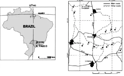
2.2. Study locations

The study fields are located in the surroundings of Araras, São Paulo State, Brazil (Fig. 1). Monthly average climatic data of Limeira station are given in Table 1. Fifteen sugarcane fields (±100 ha each), with each field comprising two to five adjacent plots were analysed. The soil in each field was sampled at two depths (0–20 and 60–80 cm) by auger at 7–16 sites and in 13 fields, one soil profile was examined in detail, as described by van den Berg and Oliveira (2000a,b). The profiles were used as reference profile for the field in which they were sited. For the two fields without profile, data were used from profiles of other fields with similar soil characteristics as judged by soil texture and chemical properties of the auger samples.

2.3. Crop data

The ‘Usina São João’ sugarcane mill provided data on planting, harvesting and fresh cane yields of 81 crops of sugarcane (cv. NA5679) on the study fields. Data on cane composition (sugars and non-soluble solid contents of fresh cane stalks) were available for 51 of these crops. These data pertain to samples taken randomly from lorries entering the mill after harvest.

2.4. The simulation model

2.4.1. General outlines

Fig. 1. Location of study region in Brazil and study fields in study region.

2.4.2. Representation of the rooted soil and initial settings

The soil as considered in the model is divided in compartments. Each compartment has a thickness of 25 cm, except the deepest one. The lower boundary of that deepest compartment represents the lower bound-ary of the rooted soil zone until it attains a thickness of 25 cm, when a new lower compartment is initialised.

Rooting depth at emergence was set to 40 cm for plant cane and to RDM for ratoon cane, i.e. it is as-sumed that the root system remains intact after harvest (c.f. Ball-Coelho et al., 1992). Downward extension

Table 1

Average monthly climate data at Limeira (22◦₃₂′_{S, 47}◦₂₇′_{WG; 639 m a.m.s.l., 1940–1990)}a

January February March April May June July August September October November December Average meant(◦C) 22.8 22.7 22.2 20.4 18.3 17.0 16.8 18.7 20.0 20.9 21.5 22.0

Average maximumt(◦_{C) 29.1 29.2 28.9 27.5 25.3 24.4 24.7 27.2 27.7 28.2 28.5 28.5}

Average minimumt(◦_{C) 18.0 18.1 17.2 14.8 12.4 11.1 10.6 12.0 13.3 14.9 15.9 17.0}

Precipitation (mm) 236 192 165 68 56 41 28 31 63 128 153 231

No. of rainy days 18 16 14 7 6 5 4 3 6 11 12 17

Bright sunshine (h) 194 181 214 213 208 195 219 226 202 208 212 178

a_{Source: Instituto Agronômico de Campinas.}

of the rooted zone is assumed to proceed at a constant rate of 1 cm per day, until it reaches depth RDM.

Initial soil water contents of each compartment were set atθ_2d (soil water content 2 days after field

satu-ration) for plant cane and at the final value under the previous crop for ratoon cane.

2.4.3. Transpiration and water withdrawal by roots Maximum transpiration rate (Tm, cm per day), i.e.

Table 2

Principal features of the crop growth model

Feature Description

Crop growth

Gross photosynthesis rate Driessen and Konijn (1992); function of intercepted radiation and light use efficiency; levels off at temperature dependent light saturation plateau Maintenance respiration rate Driessen (1997); temperature dependent mass fraction for each organ;

maintenance respiration is discounted after assimilate partitioning Conversion efficiency of primary

assimilates to plant material

Penning de Vries et al., (1989); organ specific parameters, based on biomass composition

Leaf mass and area dynamics Assimilate allocation to leaves occurs at maximum rate whenever net marginal photosynthesis gains exceed 0, and stops when gains are≤0. An

average value of specific leaf area (area per unit mass), is used to calculate leaf area index (LAI). Leaves die due to physiologic ageing. Leaf area also decreases when respiration exceeds assimilate allocation to leaves Stem growth Basic assimilate allocation to stems is proportional to assimilate allocation

to leaves. More assimilates are allocated to stems when leaf growth stops while soil water is readily available (Ta/Tm≥0.8)

Root growth Basic assimilate allocation to roots is proportional to Sroot,max−Sroot,

where Sroot,max is a target value for root biomassSroot (kg ha−1). More

assimilates can be allocated to roots when leaf growth stops and soil water status limits transpiration (Ta/Tm<0.8)

Formation and remobilization of stored reserves Reserves are formed when assimilates remain available after allocation for structural growth. Remobilization is a simple function of temperature and water availability. Stored reserves cannot exceed 0.6 of total stem biomass

Links between crop growth and water balance Gross photosynthesis rate is assumed to be linearly related toTa/Tm

Assimilate partitioning is affected (see above)

Canopy temperature rises. A linear relation is assumed between (Tm−Ta)

and increase in maximum temperature. This affects phenological devel-opment, leaf ageing and maintenance respiration

Water balance

Potential evapotranspiration rate (E0) Penman method as implemented by Driessen (1997)

Maximum transpiration rate (Tm) Driessen and Konijn (1992); function ofE0, leaf area index (LAI),

extinction coefficient for global radiationkeand a wind turbulence

factorF:Tm=E0(1−ekeLAI_)F

Actual transpiration rate (Ta) See text

Maximum evaporation rate (Em) from

wet cropped soil surface

Driessen and Konijn (1992); function ofE0, LAI (including death leaves)

and extinction coefficient for global radiation:Em=E0ekeLAI

Actual evaporation rate (Ea) Based on Supit et al. (1994), after Ritchie (1972), as function of number

of days after last rain>E0. Extraction from surface layer only

Infiltration Gauged rainfall+irrigation; not corrected for leaf interception or runoffa

Percolation and deep drainage Simple ‘tipping bucket’ approach, using field capacity concepta a_{The study soils are very permeable and there is no groundwater influence. Tensiometer readings on covered soils of the study fields}

suggest that water content decreases some 0.01 cm cm−3 _{between 2 and 5 days after field saturation (van den Berg, 1996).}

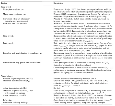
soil water status, is based on a combination of the ap-proach of Allen et al. (1998) and a free interpretation of a large number of field trials, reviewed by Gard-ner (1983). It is assumed that, from an initially wet soil, a fractionpsoilof total available soil water can be

removed before actual transpiration rate (Ta, cm per

day) drops belowTm. When the fraction of extracted

available water exceedsp_soil,T_a/T_mdecreases linearly with the amount of available water left in the soil. For this study,p_soil was determined as a function of at-mospheric demand according to Allen et al. (1998). In the model,psoil is assumed to be distributed over

Fig. 2. Schematic representation of depth dependent soil water depletion fractions.

first wilt noted by Gardner (1983). Each compartment ihas a specific soil water depletion fractionpi.

Water uptake by roots during time interval1(1 day)

is accomplished in up to N+1 steps, where Nis the number of rooted compartments. For each stepj, the compartment in which water is most readily available is presumed to be the one with the greatest value of a dimensionless variablefr,i,j, which is calculated as

fr,i,j =

θi,j −θ−1.5 MPa

(1−pi)θ2d−1.5 MPa (1)

whereθi,j is the water content of compartmenti, just before stepj, andθ−1.5 MPa the soil water retained at −1.5 MPa matric potential.

The rate of water withdrawalUi,j(cm per day) from this compartment is calculated as

Ui,j =Tmfr,i,j (2)

Ui,j was bounded by the conditions thatUi,j≤Tmand

that the amount of water withdrawn from compart-ment i may not exceed the amount that is actually available. Further water uptake from compartment i is blocked when its water content during1decreases

≥0.02 cm3cm−3. This maximum sink term (Hoogland et al., 1981) was introduced to avoid excessive water uptake from a small compartment.

Subsequently,θi,j is adjusted and the procedure is repeated for stepj+1, etc.

The model offers two options to calculateTa:

1. Ta is calculated after completion of step N+1 by integratingUi,j of Eq. (2). In this representation,

Ta is determined by the water content of the soil

compartment(s) in which water is most readily available.

2. Alternatively,Ta is calculated previously as

T_a =T_m θsoil−θ−1.5 MPa (1−psoil)θ2d−1.5 MPa

(3)

bounded by the condition T_a≤T_m, where θ_soil is

the water content averaged over the rooted part of the soil. Eqs. (1) and (2) are used in this option but the ‘loop’ is left as soon as cumulative water withdrawal during1reachesTa.

When soil water distribution is homogeneous, both options yield practically identical results as, e.g. WOFOST (Boogaard et al., 1998) and SUCROS (van Laar et al., 1997). However, option 1 yields con-siderably larger T_as when wet and dry layers occur immediately above or below each other.

2.5. Assessment of uncertainties in actual yield estimates

Cane dry matter yields (kg ha−1_{) were calculated}

for each field as the product of fresh cane yield and content of sugar+insoluble solids. Standard deviations of yields from individual plots within a field were estimated as well. If only data on fresh cane weights were available (30 cases), average dry matter yields and standard deviations of yields among adjacent plots for each harvest were approximated as

Yk = of a field at harvest k, C the average dry matter (sugar+insoluble solids) content of fresh cane stalks at harvest (0.29 kg kg−1_{),nthe number of plots in the}

field, Fi,k the mass of fresh cane stalks at plot i at harvestk(kg ha−1),Ai the surface area of ploti(ha),

plots within the field at harvest k (kg ha−1), SC the estimated standard deviation of dry matter content of fresh cane calculated from data provided by the mill (0.029 kg kg−1_{) andr}

C,F the correlation coefficient of fresh cane yield and cane dry matter content (−0.491).

2.6. Maximum rooting depths

The determination of values of RDM as input in the simulation model, is based on the following reasoning, in analogy with Jones et al. (1991).

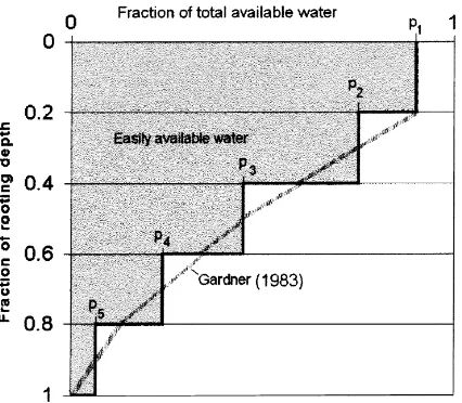
For the reference profiles, it is assumed that ‘rootability’ of a soil horizon is unaffected (i.e. 1.0) if Al3+ _{saturation is less than 40%, and nil (i.e. 0.0)} if Al3+ _{saturation exceeds 80%. An intermediate} value is taken when Al3+ _{saturation is between 40} and 80%. The rootability indices of each soil horizon are multiplied by their thickness (down to a depth of 200 cm) and summed to obtain the value of the ‘effective’ RDM.

Data from the auger samples and a pedo-transfer function were used to determine a probability density function for the assessment of errors in the represen-tativeness of calculated effective RDM values. The derivation of the pedo-transfer function is illustrated in Fig. 3, which shows effective RDM and Al3+ sat-uration of the 60–80 cm layer (Al60–80) of 31 profiles

of strongly weathered soils in south and south-east

Fig. 3. Maximum effective rootable depth (RDM) as a function of the Al3+_{saturation at 60–80 cm depth (Al}

60–80, %).

Brazil (including those from the study fields). RDM is not affected by the Al3+_{saturation of the 0–20 cm} layer, which, modified by liming, never exceeded the lower threshold value of 40%. The following relation was derived from these data to generate RDM values:

RDMi,j =aAlj,60–80+b+ε (5)

bounded by the limits 30≤RDMi,j≤200, where RDMi,j is the ith generated value of RDM for field

j (cm), Alj ,60–80 the average value of Al60–80 in

fieldj(%),a,bthe regression coefficients calculated from the data in Fig. 3 (excluding data pairs with Al60–80<25%):a=−2.565 cm and b=265.9 cm) and εa stochastic variable (cm) representing the deviation

from the mean value of RDM.

van den Berg and Oliveira (2000a) showed that Al60–80presents considerable within-field variation in

the study region, but spatial autocorrelation is weak for the sampling intervals they considered. This, and the small number of sites in each field prompted us to assume a Gaussian probability distribution for RDM, with averageε=0 and standard deviationSRDM.

Stan-dard statistical procedures (see e.g. Helstrom, 1991) were used to estimateSRDMfrom the standard

devia-tion of Al60–80 in fieldj(SAlj,60–80), the standard

de-viations of regression coefficientsaandb(Sa=1.181,

Sb=70.14) of Eq. (5), and the correlations betweena andb(ra,b=−.955)

S_RDM2 =Al2_j,60–80S_a2+a2S_Al2

j,60–80+S

2

b

+2Alj,60–80SaSbra,b (6)

SAlj,60–80was approximated by the root pooled within

field variance of Al60–80 (=14.98%). Preliminary analysis suggested that within-field values of Al60–80

have approximately normal distribution. The same was implicitly assumed for the residuals of the reg-ression equation derived from Fig. 3.

Besides, it is difficult to quantify the implications of such general statements as ‘few fine roots’.

2.7. Generating water retention data

For a data set including the study soils, van den Berg (1996) showed thatθ2d−1.5 MPaas inferred from

tensiometer readings in the field and water retention curves in the lab, is correlated with the soil’s dry bulk density and total iron content. van den Berg (1997) suggested that if these data are not available, as is the case for the auger samples in this study, an av-erage value of 0.17 cm3_cm−3 _{can be substituted for} θ_2d−1.5 MPa. He found a standard deviation (Sθ2d−1.5 MPa)

of 0.03 cm3cm−3_{. However, comparing} gravimetri-cally determined field water contents with tensiome-ter readings and lab data, suggested that the average value may be overestimated by up to 0.04 cm3_cm−3_. The model used requires input of the upper limit of available water (water stored in the soil after excess water is removed by drainage; in our case represented byθ_2d(cm3cm−3)), the lower limit of available water

(estimated atθ−1.5 MPa, cm3cm−3), and an assessment

of the water content of ‘air-dry soil’θAD(cm3cm−3).

These data were generated as follows:

1. θ2d−1.5 MPa values are obtained by assuming a normal distribution with average=either 0.17 or 0.13 cm3cm−3_andS

θ2d−1.5 MPa=0.03 cm3cm−3. To

avoid senseless data, generated values were boun-ded by 0.07 cm3cm−3_6θ

2d−1.5 MPa60.26 cm3cm−3.

2. θ−1.5 MPa, i.e. the presumed lower boundary of

available water (cm3_cm−3_{) is calculated using a} transfer function derived by van den Berg (1996) for a data set including the same soils

θ−1.5 MPa=0.02+0.27(clay+silt) (7a)

where (clay+silt) is the average content of (clay+ silt), kg kg−1_{of the soil in the field.}

3. θ2d is calculated as

θ2d =θ2d−1.5 MPa+θ−1.5 MPa (7b) 4. For the assessment of air-dry water contentsθAD, a

‘residual soil water content’θr(cf. van Genuchten,

1980) was calculated according to van den Berg (1997), as

θ_r=0.064+0.19(clay+silt)2−2.7×102C2_org (7c)

where Corgis the organic carbon content (kg kg−1).

The calculated value was bound by the limits 0≤θr≤θ−1.5 MPa−0.005. θr was assumed to be retained at a soil water potential of −10 MPa and 0.25θ−1.5 MPa was assumed to correspond with a soil water potential of−100 MPa and less. 5. Intermediate values were obtained by loglinear

in-terpolation where necessary. In the current version of the model this is only used for the assessment of water contents of air-dry soil material, i.e. in equi-librium with the atmosphere.

2.8. Independent realisations from normal distributions

Independent random samples from normal distri-butions (to generate values for RDM andθ2d−1.5 MPa)

were simulated by first generating uniformly dis-tributed random numbers with the FORTRAN RAN function and the RANØ subroutine described by Press et al. (1986). Transformation to a normal distribution was done according to Casella and Berger (1990).

2.9. Model runs

The crop model was used to calculate water-limited yield potentials of sugarcane for the following config-urations:

0 Effective RDM andθ2d−1.5 MPa obtained

from reference profiles

1 RDM calculated stochastically according to Eq. (5);θ_2d−1.5 MPa set to an average value

of 0.17 cm3_cm−3_{; method 1 for water uptake}

2 Water retention data generated stochastically; RDM set to the field average (Eq. (5);εset

to 0); method 1 for water uptake

3 As 2, but with averageθ2d−1.5 MPaset to 0.13

instead of 0.17

4 Both water retention data (averageθ2d−1.5 MPa

set to 0.17) and RDM are generated stochastically; method 1 for water uptake 5 As 4, but using method 2 for water uptake 6 As 4, but with averageθ_2d−1.5 MPaset

to 0.13 instead of 0.17

7 As 4, but disregarding uncertainties related to the use of the transfer function of Eq. (5). This reduces Eq. (6) toSRDM≈|a|SAl60–80=

The model was run 100 times for each harvest for configurations 1–7, which adds up to 7×81×100 runs (±7 h run time PC, 266 MHz). The average yield po-tential per harvest,Ysimand the pooled standard

devia-tionSY ,sim(root mean of squared standard deviations) were calculated from the results of these test runs.

3. Results

A comparison of modelled cane yield potentials and actual yield records (expressed in cane dry matter) for model configuration 0 (soil data from reference profiles) is given in Fig. 4. The correlation between recorded harvested cane dry matter yields and cal-culated water-limited cane yield potentials is highly significant, but the correlation coefficient (r2=0.43) seems rather small considering the advanced manage-ment applied. The root mean square of residuals from regression between simulated yield potentials and actual yield records is 4449 kg ha−1_{. The average}

difference between simulated yield potentials and harvested dry cane yields is 16,840 kg ha−1_{. Part of}

the difference between the 1:1 line and the trend line is due to harvest losses and cane tips and basal parts which are included in the modelled yield potentials but not in the yield records. No quantified data are available for these loss factors, but they are probably of minor importance, because harvesting is done very carefully, manually, and basal parts and cane tips are very small compared to the cane stalks of 3 m length or more. Their effect on scatter in Fig. 4 is probably even smaller.

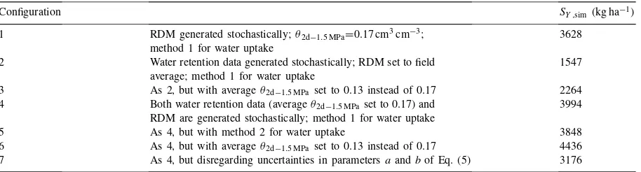
Table 3

‘Pooled’ standard deviations of calculated yield potentials (SY ,sim) for studied model configurationsa

Configuration SY ,sim (kg ha−1)

1 RDM generated stochastically;θ2d−1.5 MPa=0.17 cm3_cm−3_;

method 1 for water uptake

3628 2 Water retention data generated stochastically; RDM set to field

average; method 1 for water uptake

1547 3 As 2, but with averageθ2d−1.5 MPaset to 0.13 instead of 0.17 2264

4 Both water retention data (averageθ2d−1.5 MPaset to 0.17) and

RDM are generated stochastically; method 1 for water uptake

3994

5 As 4, but with method 2 for water uptake 3848

6 As 4, but with averageθ2d−1.5 MPaset to 0.13 instead of 0.17 4436

7 As 4, but disregarding uncertainties in parametersaandbof Eq. (5) 3176

a_{RDM: maximum rooting depth (cm);θ}

2d−1.5 MPa, available soil water retained 2 days after field saturation (cm3cm−3).

Fig. 4. Relation between simulated sugarcane yield potentials and on-farm yield records for 81 harvest on 15 fields, near Araras. Soil data obtained from reference profiles (configuration 0). Thin line is 1:1 line; bold line: regression line.

The actual yield pooled standard deviation, i.e. the square root of the pooled variance of yields among plots within a fieldS_Y2

k (Eq. (4b)) was calculated to be 2226 kg ha−1_.

Table 3 presents the pooled standard deviations of yield potentials calculated with stochastically gener-ated soil data (SY ,sim).

and 3). Calculated yield variances resulting from these two sources of uncertainty exceed the variances in recorded yields among plots and are large in relation to the root mean square of residuals from regression between simulated yield potentials and actual yield records (4449 kg ha−1_{) and the residuals from the 1:1} line.

Uncertainties in model results are not homoge-neous. For configuration 4, the smallest standard deviation among 100 runs was 67 kg ha−1 _{and the} largest 8537 kg ha−1_{. In one case, extreme values of} calculated dry cane yield potentials were 7600 and 49,800 kg ha−1_{! Fig. 5 (for configuration 4) shows}

that the propagation of uncertainties is inversely cor-related with RDM, i.e. sensitivity to RDM becomes greater when it becomes more restrictive within the range studied. Comparing the differences in SY ,sim between configurations 3 and 2 with those of 6 and 4, also shows that uncertainties increase with decreasing

θ2d−1.5 MPa.

Fig. 6 compares average model results for configu-rations 4 and 5. They are strongly correlated, but mod-elled yields for configuration 5 (method 2 for water uptake) are systematically lower, with an average dif-ference of 1500 kg ha−1_.

The average results for configurations 4 and 6, pre-sented in Fig. 7, also show predominantly systematic differences.

Fig. 5. Standard deviations of calculated sugarcane yield potentials in relation to average maximum rooting depth (RDM) in model configuration 4. Results of 100 simulation runs were used to estimate each standard deviation.

Fig. 6. Comparison of average simulated sugarcane yield poten-tials, obtained for configuration 4 (water uptake method 1: with compensatory effects) and configuration 5 (water uptake method 2: no compensatory effects).

Fig. 7. Comparison of calculated sugarcane yield potentials obtained for configuration 4 (average available water capacity=

0.17 cm3_cm−3_{), and configuration 6 (0.13 cm}3_cm−3_).

4. Discussion

Fig. 8. Simulated effect of maximum rooting depth (RDM) and available water capacity (θ2d−1.5 MPa) on yield potentials of consecutive

sugarcane crops at field 2. Day of planting: 16 February 1980; 1st ratoon, 11 July 1981; 2nd ratoon, 23 September 1982; 3rd ratoon, 13 September 1983–15 September 1984.

are plotted against RDM, for four hypothetical values ofθ2d−1.5 MPa. Most curves tend to converge with in-creasing RDM, indicating a dein-creasing sensitivity of calculated yield potential toθ2d−1.5 MPa. The

decreas-ing steepness of the curves with increasdecreas-ing RDM and with increasing θ_2d−1.5 MPa also indicates decreasing

sensitivity. However, the value of RDM where the curves level off, and the distances between the curves vary greatly among the scenarios. These variations are related to rainfall distribution, evaporative demand and other growth conditions throughout the growing season. Horizontal lines at the highest level would be expected in Fig. 8 if rainfall was sufficient and uniformly distributed, such as under drip irrigation. The divergent relations for the third ratoon are caused by an extreme drought spell during the summer of 1984, with only 59 mm rain in February/March. In ratoon cane, simulated cane yield potentials for equal values of total available water represented by the product RDM×θ2d−1.5 MPacm (e.g. RDM=50 cm,

θ2d−1.5 MPa=0.26 versus RDM=100 cm, θ2d−1.5 MPa =0.13) are generally slightly larger for smaller val-ues of θ2d−1.5 MPa. This is due to the competition

between water uptake by roots and evaporation from the soil surface. When θ2d−1.5 MPa is large, a large

proportion of infiltrating rainwater is retained in the surface layer, where it is subject to evaporation. With smaller θ_2d−1.5 MPa and deep rooting, more

infiltrat-ing rainwater will percolate to deeper layers in the root zone, where it is still available to the roots, but protected against evaporation. This interaction partly explains why uncertainties in θ2d−1.5 MPa have less effect on calculated yield potentials than uncertainties in RDM, as shown in Table 3, but a more important reason for this is that the estimated uncertainty in

θ2d−1.5 MPa is considerably less than in RDM, even thoughθ2d−1.5 MPa is estimated as a simple average

value.

availability to crops. However, soil-water availability research on strongly weathered soils has mostly been concentrated on physical soil properties, partly be-cause different crops and cultivars have different lev-els of tolerance and expensive crop monitoring field trials are necessary for quantified assessments and perhaps also because Al3+ _{research is traditionally} in the domain of soil fertility specialists, who are not commonly involved with neutron probes and TDRs for soil-water assessment. The results presented here suggest that systematic interdisciplinary research on these interactions may be rewarding.

Figs. 6 and 7 showed that using different methods to calculate water uptake or to assess available water capacity resulted primarily in systematic differences of calculated yield potentials. The differences are considerable, but the strong correlation between the results imply that it is hardly possible to select a supe-rior method on the basis of yield model results only. The hypothesis that water uptake is primarily condi-tioned by soil-water status of the wettest zone is insuf-ficiently tested. Almost all plant-soil-water research at crop level is done by wetting the entire root zone followed by drying by water withdrawal by crops. This is basically different from rain-fed conditions, where wet and dry soil parts may occur together. The question of appropriatep_soilvalues, which was not ad-dressed in this study, also deserves attention. Thomp-son (1976) suggests a fixed value of 0.5 for sugarcane, whereas Nable et al. (1999) found a value of 0.15 in a container experiment. Others prefer to determine psoil as a function of atmospheric demand according

to the method of Doorenbos and Kassam (1979) or its follow-up of Allen et al. (1998) as used in this paper.

5. Conclusions

The results suggest that, for the situations exam-ined, errors or uncertainties in the assessment of both recorded yields from farmers’ fields and the appraisal of water availability strongly affect the relation be-tween observed yields and calculated yield potentials. To improve the relevance of the model for studying the performance of rain-fed sugarcane in the region, re-search on rootability in relation to Al3+_{saturation and} its spatial variability calls for special attention in water availability studies. Uncertainties in yield calculations

tend to increase as the factor becomes more limit-ing. Then, the resulting variations may vary by several orders of magnitude, even when uncertainties in in-put variables are kept constant. Therefore, uncertainty analysis should be a standard practice in land-use sys-tems assessments, and not just a preliminary study for one or few scenarios.

Acknowledgements

The authors gratefully acknowledge the Instituto Agronômico de Campinas (IAC), for receiving the first author as a guest researcher, providing scientific and logistic support, soil laboratory analyses and weather data; and Usina São Jõao in Araras for providing crop data and logistic support during the field work on its properties.

This study would not have been possible without a fellowship from The Netherlands Foundation for the Advancement of Tropical Research (WOTRO) and fi-nancial support of the ‘Fundação para o Amparo da Pesquisa no Estado de São Paulo (FAPESP)’.

References

Allen, R.G., Pereira, L.S., Raes, D., Smith, M., 1998. Crop evapotranspiration: guidelines for computing crop water requirements. Food and Agriculture Organization of the United Nations, Rome, FAO irrigation and drainage paper 56, 300 pp. Ball-Coelho, B., Sampaio, E.V.S.B., Tiessen, H., Stewart, J.B., 1992. Root dynamics in plant and ratoon crops of sugarcane. Plant Soil 142, 297–305.

Boogaard, H.L., van Diepen, C.A., Rötter, R.P., Cabrera, J.M.C.A., van Laar, H.H., 1998. WOFOST 7.1. User’s Guide to the WOFOST 7.1 Crop Growth Simulation Model and WOFOST Control Center 1.5. DLO Winand Staring Centre, Wageningen, The Netherlands, Technical Document 52, 144 pp.

Boote, K.J., Jones, J.W., Pickering, N.B., 1996. Potential uses and limitations of crop growth models. Agron. J. 88, 704–716. Casella, G., Berger, R.L., 1990. Statistical Inference. Pacific Grove,

Wadsworth, Brooks/Cole.

de Koning, G.H.J., van Diepen, C.A., 1992. Crop production potential of the rural areas within the European Communities. IV. Potential, water-limited and actual crop production. The Netherlands Scientific Council for Government Policy, The Hague, Working document W68, 83 pp.

Driessen, P.M., 1997. Biophysical sustainability of land-use systems. In: Proceedings of the International Conference on Geo-Information for Sustainable Land Management, ITC, ISSS, Enschede, The Netherlands, Paper and software on CD-ROM. Driessen, P.M., Konijn, N.T., 1992. Land-use systems analysis. Wageningen Agricultural University, Wageningen, The Netherlands, 229 pp.

Dumanski, J., Onofrei, C., 1989. Techniques of crop yield asses-sment for agricultural land evaluation. Soil Use Manage. 5, 9–16.

Foy, C.D., 1992. Soil chemical factors limiting plant root growth. In: Hatfield, J.L., Stewart, B.A. (Eds.), Limitations to Plant Root Growth. Springer, New York, Advances in Soil Science, 19, pp. 97–149.

Furlani, P.R., Quaggio, J.A., Gallo, P.B., 1991. Differential responses of sorghum to aluminum in nutrient solution and acid soil. In: Wright, R.J., Baligar, V.C., Murrman, R.P. (Eds.), Plant–Soil Interactions at Low pH. Kluwer Academic Publishers, Dordrecht, The Netherlands, pp. 953–958. Gardner, W.R., 1983. Soil properties and efficient water use:

an overview. In: Taylor, H.M., Jordan, W.R., Sinclair, T.R. (Eds.), Limitations to Efficient Water Use in Crop Produc-tion. American Society of Agronomy, Madison, Wisconsin, pp. 45–64.

Helstrom, C.W., 1991. Probability and Stochastic Processes for Engineers. MacMillan, New York.

Hoogland, J.C., Feddes, R.A., Belmans, C., 1981. Root water uptake model depending on soil water pressure head and maxi-mum extraction rate. Acta Horticulturae 119, 123–136. Jones, C.A., Bland, W.L., Ritchie, J.T., Williams, J.R., 1991.

Simulation of root growth. In: Hanks J., Ritchie, J.T. (Eds.), Modelling Plant and Soil Systems. American Society of Agro-nomy, Madison, Wisconsin, Agronomy Monograph No. 31, pp. 91–123.

Nable, R.O., Robertson, M.J., Berthelsen, S., 1999. Response of shoot growth and transpiration to soil drying in sugarcane. Plant Soil 207, 59–65.

Penning de Vries, F.W.T., Jansen, D.M., ten Berge, H.F.M., Bakema, A., 1989. Simulation of ecophysiological processes of growth in several annual crops. IRRI, Los Baños and Pudoc, Wageningen, The Netherlands, Simulation Monographs 29, 271 pp.

Press, W.H., Flannery, B.P., Teukolsky, S.A., Vetterling, W.T., 1986. Numerical Recipes. The Art of Scientific Computing. Cambridge University Press, Cambridge, 818 pp.

Ritchie, J.T., 1972. Model for predicting evaporation from a row crop with incomplete cover. Water Resour. Res. 8, 1204–1213.

Rötter, R., Dreiser, C., 1994. Extrapolation of maize fertilizer trial results by using crop-growth simulation: results for Murang’a district, Kenya. In: Fresco, L.O., Stroosnijder, L., Bouma, J., van Keulen, H. (Eds.), The Future of the Land, Mobilising and Integrating Knowledge for Land-Use Options. Wiley, Chichester, UK, pp. 249–260.

Supit, I., Hooijer, A.A., van Diepen, C.A. (Eds.), 1994. System Description of the WOFOST 6.0 Crop Simulation Model Implemented in CGMS. Vol. 1: Theory and Algorithms. Joint Research Centre of the European Commission, Office for Official Publications of the European Communities, Luxembourg, EUR 15956, 146 pp.

Thompson, G.D., 1976. Water use by sugarcane. South African Sugar J., pages 593–600, 627-635.

van den Berg, M., 1996. Available water capacity in strongly weathered soils of south-east and southern Brazil. In: Proceedings of the XIII Latin American Congress of Soil Science, Solo-Suelo, Águas de Lindóia, São Paulo on CD-ROM. van den Berg, M., 1997. Retenção de água nos solos tropicais fortemente meteorizados do Sul e Sudeste do Brasil. In: Proc. III Simpósio de Hidráulica e Recursos H´ıdricos dos Pa´ıses de L´ıngua Oficial Portuguesa (SILUSBA), Maputo, V.2/P.2, 10 pp. van den Berg, M., Oliveira, J.B., 2000a. Variability of apparently homogeneous soilscapes in São Paulo State, Brazil. I. Spatial analysis. Brazilian J. Soil Sci. 24, 377–392.

van den Berg, M., Oliveira, J.B., 2000b. Variability of apparently homogeneous soilscapes in São Paulo State, Brazil. II. Quality of soil maps. Brazilian J. Soil Sci. 24, 393–407.

van Diepen, C.A., van der Wal, T., Boogaard, H.L., 1998. Deterministic crop growth modelling. Fundamentals and application for regional crop state monitoring and yield forecasting. In: Dallemand J.F., Perdigão, V. (Eds.), Proceedings of the 1994–1996 Results Conference Phare Multi-Country Environment Programme MARS and Environmental Related Applications (MERA) Project. Joint Research Centre of the European Commission, Luxembourg, EUR 18050 EN, pp. 201–227.

van Genuchten, M.Th., 1980. A closed form equation for predicting the hydraulic conductivity of unsaturated soils. Soil Sci. Soc. Am. J. 44, 892–898.