INTEGRATING TERRESTRIAL LIDAR WITH POINT CLOUDS CREATED FROM
UNMANNED AERIAL VEHICLE IMAGERY
Michael Leslar a *
a Teledyne-Optech, 300 Interchange Way, Vaughan, Ontario, Canada, L4K 5Z8, [email protected]
KEY WORDS: Unmanned Aerial Vehicle, Terrestrial LiDAR, Point Cloud, Data Fusion
ABSTRACT:
Using unmanned aerial vehicles (UAV) for the purposes of conducting high-accuracy aerial surveying has become a hot topic over the last year. One of the most promising means of conducting such a survey involves integrating a high-resolution non-metric digital camera with the UAV and using the principals of digital photogrammetry to produce high-density colorized point clouds. Through the use of stereo imagery, precise and accurate horizontal positioning information can be produced without the need for integration with any type of inertial navigation system (INS). Of course, some form of ground control is needed to achieve this result. Terrestrial LiDAR, either static or mobile, provides the solution. Points extracted from Terrestrial LiDAR can be used as control in the digital photogrammetry solution required by the UAV. In return, the UAV is an affordable solution for filling in the shadows and occlusions typically experienced by Terrestrial LiDAR. In this paper, the accuracies of points derived from a commercially available UAV solution will be examined and compared to the accuracies achievable by a commercially available LIDAR solution. It was found that the LiDAR system produced a point cloud that was twice as accurate as the point cloud produced by the UAV’s photogrammetric solution. Both solutions gave results within a few centimetres of the control field. In addition the about of planar dispersion on the vertical wall surfaces in the UAV point cloud was found to be multiple times greater than that from the horizontal ground based UAV points or the LiDAR data.
* Corresponding author
1. INTRODUCTION
For many years terrestrial LiDAR users, whether operating from a static or mobile platform, have found occlusions and shadows in their point clouds to be an obstacle in producing complete surface models. These shadows in the terrestrial LiDAR point clouds are the product of the perspective of the LiDAR system itself and are unavoidable. To compensate, terrestrial LiDAR users collect multiple scans from varying positions or orientations, but this does not always solve the problem. Under some circumstances, areas within the collection region are simply inaccessible from ground level. In urban areas, roofs, backyards or courtyards may be inaccessible because the owners cannot be contacted for permission to enter or do not wish to grant access. In rural areas, mountains, rivers or canyons may make access dangerous, costly or impossible.
Of course, it is possible to supplement terrestrial LiDAR data with airborne LiDAR or Photogrammetry data. These technologies have been around for some time, and do provide a solution that can provide highly accurate data. However, flying many sites with this technology can have high deployment costs, especially when the site is fairly remote. Unmanned Aerial Vehicles (UAVs) can provide the solution, as they are relatively inexpensive to buy and operate.
The concept of using UAVs for aerial photogrammetry is not new (Goinarov, 1997; Leslar, 2001), however, due to the revolution in technology that has taken place in the last decade, their use has become much more practical. Several factors have fuelled this revolution. Non-metric digital cameras have become lighter and less expensive, while still providing high-resolution imagery. Computer power continues to improve, allowing us to
process larger images in ever increasing numbers. Software for performing digital photogrammetry continually becomes ever more sophisticated. UAVs have become easier to control, capable of greater payloads and longer flight durations. By combining appropriate UAVs with appropriate high-resolution non-metric cameras and appropriate software, a fast and reliable solution is possible.
This paper will examine the accuracy with which point clouds generated from a UAV-based non-metric camera may be produced. It will use established control coordinates to compare the UAV data from a commercially available system to data from a commercially available terrestrial LiDAR system. It will also quantify the dispersion of points on both horizontal and vertical surfaces.
2. COLLECTING AND PROCESSING THE DATA
This study involves LiDAR and UAV data that was collected at the Teledyne-Optech offices in July 2014. The UAV used to collect this data was the Geo-X8000, with a flying time of up to 30 minutes and a maximum take-off weight of 5kg. The Geo-X8000 carried a Sony Nex-7 camera with a 19 mm lens and a resolution of 24 Megapixels. It was flown over the Optech building in a North-South-oriented grid pattern, collecting images at a rate of 1 frame per second, with an overlap of 60% and a sidelap of 30%.
The camera images were processed in Agisoft. The interior and exterior orientation parameters for the camera where calculated post-process by Agisoft. The exterior orientation parameters for the images were automatically determined without the aid of real-time position information, such as is found in an INS EO The International Archives of the Photogrammetry, Remote Sensing and Spatial Information Sciences, Volume XL-1/W4, 2015
file. Control information was manually picked out of the imagery and used in the calibration process. A dense point cloud consisting of 128,486,753 points was generated from the aligned and calibrated camera imagery. Figure 1 shows the UAV-generated point cloud, with the green line indicating the UAV’s trajectory over the building.
The terrestrial LiDAR data was collected with an Optech ILRIS-LR. The ILRIS-LR has a collection rate of 10,000 points per second, an angular accuracy of 80 rad and a range accuracy of 7 mm (Optech, 2014). To scan the Optech building, six separate occupation sites were required. Due to the short ranges involved in the scan and the need to ensure eye safety was maintained, the LR was used in normal-range mode only and the optional pan/tilt base was used to expand the field of view of the LiDAR.
Figure 1. Point cloud generated from aerial imagery collected by the Geo-X8000 UAV. The green line indicates the flight
path of the Geo-X8000.
Figure 2. ILRIS-LR scanner positions used to scan the Teledyne-Optech building.
The LiDAR data was processed and aligned in Polyworks IMAlign version 2014. Control points were manually extracted from the LiDAR data and Polyworks IMSurvey version 2014 was used to georeference the LiDAR data. Figure 2 shows the aligned and georeferenced LiDAR point cloud with the occupation points indicated.
3. THE CONTROL DATA
The control data used was surveyed by York University students around the Optech building in July 2012. To survey the control data a Leica 1200 GPS receiver, with a horizontal accuracy of 5mm + 0.5 ppm and a vertical accuracy of 10 mm + 0.5 ppm (Leica, 2005), was used to establish a traverse around the Optech building. The GPS receiver was referenced to the TopNext base station network through Optech’s continuously running base station.
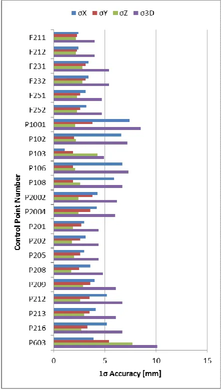
Figure 3. One-sigma accuracy estimates for control points surveyed on the Optech building.
A Leica TCA1800 total station, with an angular accuracy of 1’’ and a range accuracy of 1 mm + 2 ppm (Leica, 1999) was used to measure control points on the building and in the parking lot. The control data located on the walls and other vertical features The International Archives of the Photogrammetry, Remote Sensing and Spatial Information Sciences, Volume XL-1/W4, 2015
was computed using multiple angular observations of building features from neighbouring traverse points. The control points in the parking lot were collected on parking lot paint lines using angular measurements and slope ranges. Figure 3 shows the one-sigma accuracy estimates for the control points used to compare the LiDAR data to the point cloud generated by the UAV photogrammetry solution.
The control points used in this survey were located on the eastern side of the Optech building. These points were used since both the ILRIS and UAV point clouds cover the parking lot and several walls of the east side of the building. The control points listed in Figure 3 that start with the letter F are located on the ground in the parking lot of the building. The points that start with the letter P are located on walls of the Optech building.
4. CALCULATION OF POINT RESIDUALS
Assuming that the control points gathered by the Total Station represent the true values for the location of the building features and parking lot paint lines, it is possible to form residuals that will tell us how well the LiDAR and the UAV data conform to reality. Using primitive geometry to calculate estimates for the exact location of the geometric features, the point picking error from each point cloud may be minimized. Figure 4 shows the magnitude of the resultant residuals when the LiDAR point cloud is compared to the control field.
Figure 4. Residuals calculated from comparing aligned and georeferenced ILRIS-LR data to a control field.
The residuals in Figure 4 were broken down into the horizontal and vertical components for each control point-LiDAR pairing. It was found that the horizontal components of the control point-LiDAR residuals had a mean average of 34 mm and a standard deviation of 10 mm. The vertical component of the control point-LiDAR residuals fit better, with a mean average of 16 mm and a standard deviation of 11mm.
Figure 5. Residuals calculated from comparing aligned and georeferenced Geo-X8000 data to a control field.
Similarly, Figure 5 shows the magnitude of the resultant residuals when the UAV point cloud is compared to the control field. Again, the residuals were broken down into the horizontal and vertical components for each control point-UAV pairing. It was found that the horizontal components of the control point-UAV residuals had a mean average of 65 mm and a standard deviation of 21 mm. The vertical component of the control point-UAV residuals fit better, with a mean average of 41 mm and a standard deviation of 26 mm.
5. ESTIMATING POINT DISPERSION
A standard technique for estimating the random noise in a point cloud is by plane-fitting samples of known flat surfaces and examining the fitting statistics (Skaloud and Lichti, 2006; NATO, 2011; Olsen, 2013). In mobile applications this can give information about the boresight of the LiDAR system to its inertial navigation system. In static LiDAR, this can give information on the range accuracy of the LiDAR’s rangefinder. Therefore, 42 randomly chosen sites were selected such that The International Archives of the Photogrammetry, Remote Sensing and Spatial Information Sciences, Volume XL-1/W4, 2015
each point cloud (LiDAR and UAV) had sufficient coverage to provide at least 1000 points for planar fitting. Each plane was fit to an area of the point clouds covered by a 0.5 m radius patch. These 42 randomly selected flat surfaces covered both vertical wall surfaces and horizontal ground surfaces.
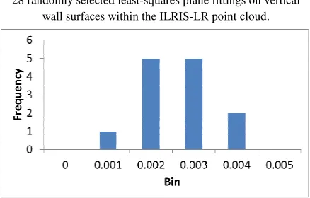
Figure 6 shows a histogram of the standard deviations of 28 planes, extracted from vertical wall surfaces in the ILRIS-LR data set. Figure 7 shows a similar histogram of the standard deviations of 14 more planes, extracted from horizontal ground surfaces in the ILRIS-LR data set. For all 42 planar surface extractions, the mean of the planar fit was zero and the estimated root mean squared (RMS) value equalled the one-sigma standard deviation value, indicating a normal distribution. In both cases the ILRIS returned one-sigma standard deviation values at or around 8 mm. This is consistent with the accuracy specifications from the manufacturer (Optech, 2014).
Figure 6. Histogram of one-sigma standard deviation values for 28 randomly selected least-squares plane fittings on vertical
wall surfaces within the ILRIS-LR point cloud.
Figure 7. Histogram of one-sigma standard deviation values for 14 randomly selected least-squares plane fittings on horizontal
ground surfaces within the ILRIS-LR point cloud.
Similarly, Figure 8 shows a histogram of the standard deviations of 28 planes, extracted from vertical wall surfaces in the Geo-X8000 data set and Figure 9 shows a histogram of the standard deviations of 14 more planes, extracted from horizontal ground surfaces in the same data set. As with the ILRIS-LR point cloud, the Geo-X8000 point cloud was able to produce 42 fitted planes with a mean average of zero and an RMS value equal to the one-sigma standard deviation value. Unlike the ILRIS data, which showed a very tight correspondence between plane statistics from vertical surfaces and plane statistics from horizontal surfaces, the Geo-X8000 had a wide discrepancy between these statistics. The Geo-X8000 had a median plane standard deviation on vertical
surfaces of around 30 mm but a median plane standard deviation on horizontal surfaces of 5 mm.
Figure 8. Histogram of one-sigma standard deviation values for 28 randomly selected least-squares plane fittings on vertical
wall surfaces within the Geo-X8000 point cloud.
Figure 9. Histogram of one-sigma standard deviation values for 14 randomly selected least-squares plane fittings on horizontal
ground surfaces within the Geo-X8000 point cloud.
6. DISCUSSION
The residual analysis shows that, quantitatively, the size of the residuals in Figure 4 and Figure 5 are quite similar. That being said, the mean average for the horizontal component of the residuals from the LiDAR (34 mm) was roughly half as large as the mean average for the horizontal component of the residuals from the UAV (64 mm). This is while the spread of the selected points from both data sets remained similar. In the horizontal direction, we can roughly equate the capabilities of the photogrammetry solution and the LiDAR solution.
On the other hand, the mean average of the vertical component of the residuals from the LiDAR data (16 mm) was significantly smaller than the vertical component of the residuals from the UAV data (41 mm). The spread on the UAV data residuals was also higher, indicating that the estimates elevations of these points were much less certain.
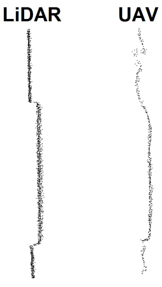
It should be stated that selecting control features, especially on the vertical surfaces was extremely difficult in the UAV point cloud. Edges, upon which, the control was located, such as window corners, were significantly rounded. Figure 10 shows a typical cross section of a window on the eastern wall of the building. The LiDAR cross section shown in Figure 10 is a realistic representation of the recessed window. The inner and outer edges of the recessed window in the LiDAR cross section are clearly defined. The UAV cross section shown in Figure 10 The International Archives of the Photogrammetry, Remote Sensing and Spatial Information Sciences, Volume XL-1/W4, 2015
contains numerous places where edges and even wall surfaces are not defined. Due to the perspective of the camera from the aerial platform, the window’s top corners are not defined at all. The bottom corner that the camera could see does have some definition, however, the actual corner is rounded and the depth of the window is variable. This is true of most corners in the UAV point cloud.
Figure 10. Typical cross section of a window in both a LiDAR point cloud and a point cloud from the UAV
Checking the dispersion of the points in the UAV point cloud we see from Figure 9 that the individual elements of the point cloud on the ground are very tightly packed. When comparing the dispersion of the ground-based points in the UAV data we find that they are comparable to the dispersion of points in both the vertical and horizontal objects from the LiDAR data (Figures 6 and 7). The dispersion shown by the UAV data on the walls of the building (Figure 8) is in stark contrast to that of both the ground-based UAV data and the LiDAR data. The dispersion of the UAV data on the vertical surfaces of the wall is nearly three to four times that of when it is on ground. This is likely due to the obliqueness of the incident angles of the rays entering the camera from the wall. The rays entering the camera from the ground surface do so at an incidence angle that is nearly perpendicular to the camera’s imaging plane.
7. CONCLUSIONS
The point cloud generated from stereo pairs of close range aerial images is tolerably close enough to the accuracy of the aligned and georeferenced LiDAR data to make them compatible. The UAV point cloud was found to be less accurate than the LiDAR point cloud and several of its surfaces have larger point dispersion on planar surfaces than the LiDAR data. However, under the correct conditions, where the camera angle was perpendicular to the target object, the accuracy and
dispersion of the UAV data was very close to that of the LiDAR data. Therefore as a means of augmenting the LiDAR data and filling the shadows and occlusions that occur due to the LiDAR’s perspective, a camera-mounted UAV solution is quite acceptable.
Goinarov, A.R., 1997, The Acquisition of Photographs Using a Radio Control Model Helicopter for Aerial Photogrammetry. A thesis submitted to Ryerson University in partial fulfilment of the degree of Bachelor of Engineering. Ryerson University, 350 Victoria Street, Toronto, Canada, M5B 2K3.
Leica Geosystems AG, 1999, LEICA T1800 • TC1800 • TCA1800 Technical Data, Heerbrugg, Switzerland,
http://www.jysklandmaaling.dk/Leica%20TCA1800.pdf (23
Jun. 2015)
Leica Geosystems AG, 2005, Leica GPS1200+ Series High performance GNSS System, Heerbrugg, Switzerland,
http://www.leica-geosystems.com/downloads123/zz/gps/general/brochures/GPS1
200_brochure_en.pdf (23 Jun. 2015).
Leslar, M., 2001, The Use of Unmanned Aircraft in Vehicle Collision Reconstruction. A thesis submitted to Ryerson University in partial fulfilment of the degree of Bachelor of Engineering. Ryerson University, 350 Victoria Street, Toronto, Canada, M5B 2K3.
NATO Science and Technology Organization, 2011, RTO-TR-SET-118 - 3D Modelling of Urban Terrain, Chapter 4 - From Point Clouds to 3D Models. Presented at Final Report of Task Group SET-118, pp. 4-14.
Optech Incorporated, 2014, ILRIS Terrestrial Laser Scanner – Summary Specification Sheet, Vaughan, Canada, www.teledyneoptech.com/wp-content/uploads/ILRIS-LR-Spec-Sheet-140730-WEB.pdf (23 Jun. 2015).
Olsen, M., 2013, Report 748 - Guidelines for the Use of Mobile LiDAR in Transportation Applications, National Cooperative Highway Research Program, Washington DC, pp. 48.
Skaloud, J. and Lichti, D. 2006, Rigorous approach to bore-sight self-calibration in airborne laser scanning. ISPRS Journal of Photogrammetry & Remote Sensing, vol 61 (2006), pp. 47-– 59.