Sr. No
Topic
1.
Scope of the Journal
2.
The Model
3.
The Advisory and Editorial Board
4.
Papers
First Published in the United States of America. Copyright © 2012
Foundation of Computer Science Inc.
International Journal of Computer Applications (IJCA) creates a place for publication of papers which covers the frontier issues in Computer Science and Engineering and their applications which will define new wave of breakthroughs. The journal is an initiative to identify the efforts of the scientific community worldwide towards inventing new-age technologies. Our mission, as part of the research community is to bring the highest quality research to the widest possible audience. International Journal of Computer Applications is a global effort to consolidate dispersed knowledge and aggregate them in a search-able and index-able form.
The perspectives presented in the journal range from big picture analysis which address global and universal concerns, to detailed case studies which speak of localized applications of the principles and practices of computational algorithms. The journal is relevant for academics in computer science, applied sciences, the professions and education, research students, public administrators in local and state government, representatives of the private sector, trainers and industry consultants.
Indexing
International Journal of Computer Applications (IJCA) maintains high quality indexing services such as Google Scholar, CiteSeer, UlrichsWeb, DOAJ (Directory of Open Access Journals) and Scientific Commons Index, University of St. Gallen, Switzerland. The articles are also indexed with SAO/NASA ADS Physics Abstract Service supported by Harvard University and NASA, Informatics and ProQuest CSA Technology Research Database. IJCA is constantly in progress towards expanding its contents worldwide for the betterment of the scientific, research and academic communities.
Topics
Open Review
International Journal of Computer Applications approach to peer review is open and inclusive, at the same time as it is based on the most rigorous and merit-based ‘blind’ peer-review processes. Our referee processes are criterion-referenced and referees selected on the basis of subject matter and disciplinary expertise. Ranking is based on clearly articulated criteria. The result is a refereeing process that is scrupulously fair in its assessments at the same time as offering a carefully structured and constructive contribution to the shape of the published paper.
Intellectual Excellence
The current editorial and Advisory committee of the International Journal of Computer Applications (IJCA) includes members of research center heads, faculty deans, department heads, professors, research scientists, experienced software development directors and engineers.
Dr. T. T. Al Shemmeri, Staffordshire University, UK Bhalaji N, Vels University
Dr. A.K.Banerjee, NIT, Trichy Dr. Pabitra Mohan Khilar, NIT Rourkela Amos Omondi, Teesside University Dr. Anil Upadhyay, UPTU
Dr Amr Ahmed, University of Lincoln Cheng Luo, Coppin State University Dr. Keith Leonard Mannock, University of London Harminder S. Bindra, PTU
Dr. Alexandra I. Cristea, University of Warwick Santosh K. Pandey, The Institute of CA of India Dr. V. K. Anand, Punjab University Dr. S. Abdul Khader Jilani, University of Tabuk Dr. Rakesh Mishra, University of Huddersfield Kamaljit I. Lakhtaria, Saurashtra University Dr. S.Karthik, Anna University Dr. Anirban Kundu, West Bengal University of
Technology
Amol D. Potgantwar, University of Pune Dr Pramod B Patil, RTM Nagpur University Dr. Neeraj Kumar Nehra, SMVD University Dr. Debasis Giri, WBUT
Dr. Rajesh Kumar, National University of Singapore Deo Prakash, Shri Mata Vaishno Devi University Dr. Sabnam Sengupta, WBUT Rakesh Lingappa, VTU
D. Jude Hemanth, Karunya University P. Vasant, University Teknologi Petornas Dr. A.Govardhan, JNTU Yuanfeng Jin, YanBian University Dr. R. Ponnusamy, Vinayaga Missions University Rajesh K Shukla, RGPV
Dr. Yogeshwar Kosta, CHARUSAT Dr.S.Radha Rammohan, D.G. of Technological Education
T.N.Shankar, JNTU Prof. Hari Mohan Pandey, NMIMS University Dayashankar Singh, UPTU Prof. Kanchan Sharma, GGS Indraprastha
Vishwavidyalaya
Bidyadhar Subudhi, NIT, Rourkela Dr. S. Poornachandra, Anna University Dr. Nitin S. Choubey, NMIMS Dr. R. Uma Rani, University of Madras Rongrong Ji, Harbin Institute of Technology, China Dr. V.B. Singh, University of Delhi
Anand Kumar, VTU Hemant Kumar Mahala, RGPV
Prof. S K Nanda, BPUT Prof. Debnath Bhattacharyya, Hannam University Dr. A.K. Sharma, Uttar Pradesh Technical
University
Dr A.S.Prasad, Andhra University
Rajeshree D. Raut, RTM, Nagpur University Deepak Joshi, Hannam University Dr. Vijay H. Mankar, Nagpur University Dr. P K Singh, U P Technical University Atul Sajjanhar, Deakin University RK Tiwari, U P Technical University Navneet Tiwari, RGPV Dr. Himanshu Aggarwal, Punjabi University
Ashraf Bany Mohammed, Petra University Dr. K.D. Verma, S.V. College of PG Studies & Research Totok R Biyanto, Sepuluh Nopember R.Amirtharajan, SASTRA University
Sheti Mahendra A, Dr. B A Marathwada University Md. Rajibul Islam, University Technology Malaysia Koushik Majumder, WBUT S.Hariharan, B.S. Abdur Rahman University Dr.R.Geetharamani, Anna University Dr.S.Sasikumar, HCET
Rupali Bhardwaj, UPTU Dakshina Ranjan Kisku, WBUT Gaurav Kumar, Punjab Technical University A.K.Verma, TERI
Prof. B.Nagarajan, Anna University Vikas Singla, PTU
Dr H N Suma, VTU Dr. Udai Shanker, UPTU
Anu Suneja, Maharshi Markandeshwar University Prof. Rachit Garg, GNDU
Prof. Surendra Rahamatkar, VIT Prof. Shishir K. Shandilya, RGPV
M.Azath, Anna University Liladhar R Rewatkar, RTM Nagpur University R. Jagadeesh K, Anna University Amit Rathi, Jaypee University
Dr. Dilip Mali, Mekelle University, Ethiopia. Dr. Paresh Virparia, Sardar Patel University Morteza S. Kamarposhti , Islamic Azad University
of Firoozkuh, Iran
Dr. D. Gunaseelan Directorate of Technological Education, Oman
Dr. M. Azzouzi, ZA University of Djelfa, Algeria. Dr. Dhananjay Kumar, Anna University Jayant shukla, RGPV Prof. Yuvaraju B N, VTU
Dr. Ananya Kanjilal, WBUT Daminni Grover, IILM Institute for Higher Education Vishal Gour, Govt. Engineering College Monit Kapoor, M.M University
Dr. Binod Kumar, ISTAR Amit Kumar, Nanjing Forestry University, China. Dr.Mallikarjun Hangarge, Gulbarga University Gursharanjeet Singh, LPU
Dr. R.Muthuraj, PSNACET Mohd.Muqeem, Integral University Dr. Chitra. A. Dhawale, Symbiosis Institute of
Computer Studies and Research
Dr.Abdul Jalil M. Khalaf, University of Kufa, IRAQ.
Dr. Rizwan Beg, UPTU R.Indra Gandhi, Anna University V.B Kirubanand, Bharathiar University Mohammad Ghulam Ali, IIT, Kharagpur Dr. D.I. George A., Jamal Mohamed College Kunjal B.Mankad, ISTAR
Raman Kumar, PTU Lei Wu, University of Houston – Clear Lake, Texas. G. Appasami , Anna University S.Vijayalakshmi, VIT University
Dr. Gurpreet Singh Josan, PTU Dr. Seema Shah, IIIT, Allahabad Dr. Wichian Sittiprapaporn, Mahasarakham
University, Thailand.
Chakresh Kumar, MRI University, India
System Progress Estimation in Time based Coordinated Checkpointing Protocols Authors : P. K. Suri, Meenu Satiza
1-6
Adaptive Learning for Algorithm Selection in Classification Authors : Nitin Pise, Parag Kulkarni
7-12
Routing Protocol for Mobile Nodes in Wireless Sensor Network Authors : Bhagyashri Bansode, Rajesh Ingle
13-16
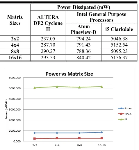
32-Bit NxN Matrix Multiplication: Performance Evaluation for Altera FPGA, i5 Clarkdale, and Atom Pineview-D Intel General Purpose Processors
Authors : Izzeldin Ibrahim Mohd, Chay Chin Fatt, Muhammad N. Marsono
17-23
Recognizing and Interpreting Sign Language Gesture for Human Robot Interaction Authors : Shekhar Singh, Akshat Jain, Deepak Kumar
24-31
Change Data Capture on OLTP Staging Area for Nearly Real Time Data Warehouse base on Database Trigger
Authors : I Made Sukarsa , Ni Wayan Wisswani, K. Gd. Darma Putra, Linawati
32-37
Decision Support System for Admission in Engineering Colleges based on Entrance Exam Marks Authors : Miren Tanna
38-41
A Genetic Algorithm based Fuzzy C Mean Clustering Model for Segmenting Microarray Images Authors : Biju V G, Mythili P
42-48
System Progress Estimation in Time based Coordinated
Checkpointing Protocols
P. K. Suri
Dean, Research and
Development; Chairman, CSE/IT/MCA, HCTM Technical Campus, Kaithal,Haryana, India
Meenu Satiza
HCTM Technical Campus
ABSTRACT
A mobile computing system consists of mobile and stationary nodes. Checkpointing is an efficient fault tolerant technique used in distributed systems. Checkpointing in mobile systems faces many new challenges such as low wireless bandwidth, frequent disconnections and lack of stable storage on mobile nodes. Coordinated Checkpointing that minimizes the number of processes to take useless checkpoints is a suitable approach to introduce fault tolerance in such systems. The time-based checkpointing protocol eliminates communication overheads by avoiding extra control messages and useless checkpoints. Such protocols directly accesses stable storage when checkpoints are saved. In this paper a new probabilistic approach for evaluation of the system progress is devised which is suitable for the mobile distribution applications. The system behavior is observed by varying some system parameters such as fault rate, clock drift rate, saved checkpoint time, checkpoint intervals. A validation regarding system progress is made via a simulation technique. The simulation results show that the proposed probabilistic model is well suited for the mobile computing systems.
General Terms
Checkpointing, System progress, Simulation
Keywords
Distributed system, fault tolerance, time-based checkpointing
System progress, consistent checkpoint
1.
INTRODUCTION
Checkpointing is a major technique of fault tolerance system in which state of a process has to be saved in stable storage so that the process can be restarted in case of fault. There are two main categories of checkpointing techniques: (i) coordinated and (ii) uncoordinated checkpointing. In coordinated checkpointing, the processes send the control messages to their dependent processes to save their states at the same time. This results a global consistent state from which the system recovers when a fault occur in the system. In uncoordinated checkpointing, the processes save their states independently. In this type of protocol, during fault occurrence processes rollback to a point of recovery. Recently new type of time based coordinated checkpointing techniques have been introduced which avoid extra coordination messages among dependent processes. The time based approach is based on loosely synchronized timers. The Timer information is piggybacked along application messages. System performance of the time based checkpointing protocols depends on the
application and system’s characteristics such as checkpoint intervals, save checkpoint time, resynchronize time, clock drifts. We proposed a probabilistic model for the system
progress with particular system parametric values. This model shows that how system operations can affect the system performance and the simulation results shows the states at which system perform well with the particular values of defined parameters. A simulation model is also developed to validate the system progress.
1.1
Related work
In 1985, Chandy and Lamport [1] proposed a global snapshot algorithm for distributed systems. The global state is achieved by coordinating all the processors and logging the channel state at the time of checkpointing. Special messages called markers are used for coordination and for identifying the messages originating at different checkpointing intervals. In 1987, Koo-Toueg [5] proposed a two phase Minimum-process Blocking Scheme for distributed system. The consequence of algorithm is a consistent global checkpointing state that involves only the participating processes and prevent live lock problem (A single failure can cause an infinite rollbacks)
In 1996 Ravi Prakash and Mukesh Singhal [11] presented a synchronous non-blocking snapshot collection algorithm for mobile systems that does not force every node to take a local snapshot. They had also proposed a minimal rollback/recovery algorithm in which the computation at a node is rolled back only if it depends on operations that have been undone due to the failure of node(s).
In 1996 N. Neves and W.K.Fuches [9] presented a time based checkpointing protocol which eliminate communication overhead present in traditional checkpointing protocols. The checkpointing protocol was implemented on CM5 and their performance was compared using several applications. In 2001 Guohong Cao and Mukesh Singhal [4] had introduced the concept of “mutable checkpoint” which is neither a tentative checkpoint nor a permanent checkpoint. To design efficient checkpointing algorithms for mobile computing systems the mutable checkpoints can be saved anywhere e.g. the main memory or local disk of MHs. In this way taking a mutable checkpoint avoids the overhead of transferring large amounts of data to the stable storage at MSSs over the wireless network.
In 2002 Chi-Yi Lin et. al. [7] proposed an improved time based checkpointing protocol by integrating the improved timer synchronization technique. The mechanism of time synchronization utilizes the accurate timer in MSSs as an absolute reference. The timers in fixed hosts (MSSs) are more reliable than those in MHs.
system each process takes a soft checkpoint first which is saved in main memory of mobile hosts. If the process is irrelevant to initiator it can be discarded otherwise will be saved in the local disk at a later time as hard checkpoint. As a result the number of disk accesses in mobile hosts can be reduced. The advantage of using time based approach improves the need of explicit coordination message.
In 2006 Men Chaoguang [2] proposed a two-phase time based checkpointing strategy. This eliminates orphan and in-transit messages. In this strategy, the issues of time - based adaptive checkpoint strategy was evaluated which describes about all processes need not to block their computation work and also not to log all messages. In proposed strategy the inconsistency issues are also discussed.
In 2007 Awasthi and Kumar [6] had proposed a probabilistic approach based on keeping track of direct dependencies of processes. Initiator MSS collects the direct dependency vectors of all processes and sends the checkpoint request to all dependent MSSs. This step was taken to reduce the time to collect the coordinated checkpoint. It would also reduce the number of useless checkpoints and the blocking of the processes. The buffering of selective messages at the receiver end and exact dependencies among processes had maintained. Hence the useless checkpoint requests and the number of duplicate checkpoint requests get reduced.
In 2008 Suchistmita Chinara and Santanu Kumar Rath [3] had proposed an energy efficient mobility adaptive distributed clustering algorithm for Mobile ad-hoc Network. In which a better cluster stability and a low maintenance overhead is achieved by volunteer and non volunteer cluster heads. The proposed algorithm is divided into parts like cluster formation, energy consumption model, cluster maintenance. The objective of algorithm is to minimize the re affiliation rate (A changing situation of member node search for another head is called re affiliation) .The simulation Experiment compare the ID of members. A high ID member act as cluster head and cluster maintenance overhead is reduced from time to time.
In 2011 Anil Panghal, Sharda Panghal, Mukesh Rana [10] presented a comprehensive study of the existing techniques namely Checkpoint-based recovery and Log-based recovery. Based on the study they conclude that Log-based recovery techniques which combine checkpointing and logging of nondeterministic events during pre-failure execution are suitable for systems that frequently interact with the outside world. They also conclude that communication-induced checkpointing reduces the message overhead if implemented along with checkpoint staggering can prove to be the best method for recovery in distributed systems
2.
PROBLEM FORMULATION
In this paper a number of time based checkpointing protocols are analyzed. In [9] Neves and Fuchs had given the concept of timers to reduce the communication overhead. They made the following assumptions:
(a) The processes involved in checkpointing have loosely synchronized clocks.
(b) All the processes are approximately synchronized and have a deviation from real time in their local clock timers. The local clock drift rate between the processes
being assumed as ρ.
(c) The timer will terminate at most (2ρT/ (1-ρ2) ≈ 2ρT) seconds apart. Here T is the initial timer value. Normally
drift rate ρ attains values between 10-5
sec. to 10-8 sec.
(d) The clocks will show a maximum drift of 2NρT after N checkpoint interval.
Consider the following figure1. in which P1 and P2 are two processes. The message M1 is sent from process P1 to P2 in its Nth checkpoint interval and also message M2 is being sent in same interval of P1 to (N+1)th interval of P2. Let some fault arrives in timeline of Process P2.
It is observed that checkpoint N+1 is saved in P2 before the fault occurrence. Now P2 has yet to receive M2. But P2 has no information of message M2. Such situations can be handled by resending unacknowledged messages again.
According to Neves the more time is wasted in storing checkpoints and the processes has to block its execution for a long time which is an impractical situation. Such inconsistencies of in-transit or orphan messages can be handled by using time based checkpointing approach where the messages are now being sent along with timers.
According to Men Chaoguang approach [2] the orphan messages can be eliminated by using communication induced approach and in-transit messages can be stored in message logging queue. The following figure 2. Illustrates the above situations.
Consider P1 and P2 are two processes. T1 and T2 are their
timers respectively. Let MD = D + 2 ρ T be the maximum
deviation between the timer of two processes = T1– T2 .tmax is the maximum delivery time at which process P2 should get the message M1. tmin is the minimum delivery time of message M4. ED = MD – tmin is the effective deviation in which the processes cannot send or receive the message .M2 and M3 lies in effective deviation and they arise the inconsistency due to orphan and in-transit messages. To handle orphan message M3 a communication induced checkpoint is placed before the delivery of message M3 and in-transit message M2 can be retrieved from message logging queue.
It is observed that the parametric values ρ, T, D, tmin, tmax,
fault rate λ, Saved checkpoint point time S, time (t) at which fault occurs affects the mobile distributed system performance.
In this paper a probabilistic model is developed in which the system performance is evaluated by varying various system parametric values.
P1
P2
M1 M2
N N+1
N N+1
Fault arrived
3.
SYSTEM PROGRESS EVALUATION
3.1
Probabilistic model development
When faults occur in the system, resynchronization is made.
Here the system’s progress is defined as the ratio of
constructive computational work to the total work during a given interval of time.
In order to perform a simulation experiment on distributed
system a random sample of time t1,t2,t3………..tn is
generated by transforming n uniform random numbers
u1,u2,u3……un in the interval (0,1).Where λ is the positive
constant depending on characteristics of distributed system [12]. The general term of time tk is
tk = –(1/λ)*logeuk where k Є [1,n] Let ts = time to store checkpoint, tmin be the minimum checkpoint delivery time, tmax be the maximum checkpointing delivery time, Tdiff be the maximum difference between timers of different processes, L be the length of checkpoint intervals before resynchronization, ρ be the clock drift rate between the processes, fr be the fault rate, Tw be the probabilistic wasted time of fault occurrence ,Twr be the probabilistic wasted time of fault occurrence between resynchronization, tr be the resynchronization time.
Let T1, T2, T3………Tnmax are n checkpoint intervals between resynchronization. When fault not occurs then this time will be equal to maximum number of checkpoint intervals nmax.
The system progress is evaluated by developing following probabilistic model.
Here ts ≤ (Tdiff + 2*nmax*L* ρ – tmin) (ts + tmin – Tdiff)/ (2*L*ρ) ≤ nmax nmax = ceil ((ts + tmin –Tdiff)/(2*L*ρ)
Let Tcons be the time interval during which constructive computational work is done. Where Tcons is given as
Tcons = L – ts – tk where k Є [1,n]
The probability density function of occurrence of fault is given as
Let Ir = Expected number of intervals between resynchronization = Probability of happening fault during any
Interval less than nmax + Probability of happening no fault during any interval less than nmax.
In Fig. 3 a set of nmax checkpoints numbers ({1, 2, 3 ……k, k+1…nmax}) are considered on the time line of the process.
The probability of a fault occurring in the kth checkpoint interval Pr[k] in last resynchronization process is given as
Pr[k] = e – fr* L*k– e – fr* L*(k+1) (nmax – 1)
Ir =
∑
k * Pr[k] + nmax * e – fr* L*k k =1Ir = (1 – e – fr* L*nmax)/ (e fr* L– 1)
Probability of wasted time of occurrence of fault Tw and the wasted time of occurrence between resynchronization Twr is given as
Tw = ((e – fr*Tcons)*( – fr * Tcons – 1 ) + 1)/(fr*(1 – e – fr*Tcons
))
The Probability of wasted time of occurrence between resynchronization Twr is given as
Twr = (1 – e – fr* L*nmax)*( ts +Tw) + e – fr* L*nmax * tr Let probability of total time between resynchronization is Tr .
Where Tr = Ir * L + Twr
Let TCW be the Probability of time used in constructive work between resynchronization
TCW = Ir*Tcons
The System Progress (SP say) of a process = TCW/Tr
The System Progress of all the processes = ∑ TCW/Tr
The System Progress of the complete system having n processes = (∑ TCW/Tr)/n.
3.2 Validation of system progress
To confirm the correctness of system progress evaluation, system progress validation is implemented to more detailed confidence level of simulation. Here in the simulation technique to achieve the validation having a better confidence level ,first 1000 runs of simulation experiment are made from 10 samples with 100 checkpoint intervals then
2000,3000,……..10000 runs are made and then average value of system progress, their standard deviation (say SD), upper ( say UL) , lower (say LL) confidence limit of system progress is computed. Further corresponding interval of interest Tcons and then corresponding optimal system progress is evaluated for the system by using the variation among the parameters
say λ, ρ, ts, fr, L. The used simulation technique follows as
Let’s take n independent samples of time interval Length L and according to such n samples values of System progress SP1,SP2,SP3………SPn .Then their mean and
P1
P2
M1
tmax
T2
T1
M2
M3
M4
tmin
ED MD
Fig.2 Elimination of inconsistent state
Fig 3. Fault arrival in kth checkpoint interval
L 2
1 k k+1
Fault Waste
standard deviation σ are evaluated .The sample mean of all
System progresses are to be evaluated by using formula:
SPmean = ∑ SPi/ n
The variance σ2
can be estimated as :
σ2
est = (1/ (n-1))*∑(SPk– SPmean) 2
The general relationship between the parameters is given as
Pr { –t ≤ SPmean≤ + t} = 1 –α
where t is the tolerance on either side of mean within which the estimated to fall within probability 1– α. The normal
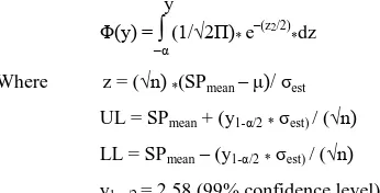
density function is Φ(y) = y1-α/2, the upper confidence limit UL and lower confidence limit LL of System progress can be obtained respectively.
y
Φ(y) =
∫
(1/√2Π)* e– (z2/2)*dz –α
Where z = (√n) *(SPmean – )/σest UL = SPmean + (y1-α/2 * σest) / (√n) LL = SPmean– (y1-α/2*σest) / (√n) y1-α/2 = 2.58 (99% confidence level)
The interval (UL - LL) will contain the true mean with a specific certain experimental confidence value [12].
3.2
Simulation results
Simulation result shows that the System Performance is affected by the various factors such as number of checkpoint intervals, Clock drift rate of processors, Fault rate of processors, Time of saving checkpoints .In our simulation experiment such variations of factors against System Progress are shown in tabular as well as graphical form.
3.2.1
Checkpoint interval vs. system progress
The following table expresses the parametric values used in proposed model. The first column shows when varying values of Fault rate (Table 4), Drift rate (Table 5), Checkpoint intervals (Table 2) and second and third column shows the corresponding other variable names and their particular values.
Table 1: Parametric values of System model
According to these values the system progress is evaluated and respective graphs are drawn. First according to increasing values of checkpoint intervals (L) corresponding decreasing values of system progress is evaluated i.e. obviously as number of checkpoint intervals are increased corresponding system progress get decreased (Fig 4) i.e. The system progress is affected by number of checkpoints
Table 2. Checkpoint intervals vs. System Progress
Checkpoint Intervals( L)
System Progress SP
100 0.9925
10100 0.950282 20100 0.902832 30100 0.857017 40100 0.81285 50100 0.770316
Fig 4: Checkpoint intervals vs. System Progress
3.2.2
Saved Checkpoint time vs. system progress
Table 3. describes as time to save checkpoints get increased the system progress get decreased.
This is illustrated in Fig.5 which is obviously true as the time to save checkpoint get increased the system progress will decrease.
Table 3. Saved Checkpoint time vs. System Progress
Saved checkpoint Time (ts)
System Progress (SP)
1 0.98183
2 0.981554
3 0.981278
4 0.980999
5 0.980723
6 0.980441
7 0.980166
8 0.979887
9 0.979609
10 0.979331
11 0.979053
12 0.978775
13 0.978498
14 0.978221
15 0.977942
SYSTEM PROGRESS EVALUATION Used System parameters Variable tr 0.1 State Tdiff 0.01
tmin 0.001
fr L 3600
Fault rate ts 0.7
ρ 0.000001
ρ fr 0.00001
Drift rate L 3600
ts 0.7
L fr 0.00001
Ckeckpoint
Interval ρ 0.000001
Fig 5: Checkpoint intervals vs. System Progress
3.2.3
Fault Rate vs. system progress
This subsection describes how fault rate affects the system progress.
Table 4. describes as fault rate get increased The system progress get decreased.This is illustrated in Fig.6
Table 4. Fault Rate vs. system progress
Fault Rate fr
System Progress SP 1.00E-16 0.999803
1.00E-15 0.999741
1.00E-14 0.999767
1.00E-13 0.999783
1.00E-12 0.999802
1.00E-11 0.999761
1.00E-10 0.999726
1.00E-09 0.999765
1.00E-08 0.999658 1.00E-07 0.999625
Fig 6 Fault Rate vs. System Progress
3.2.4
Drift Rate vs. system progress
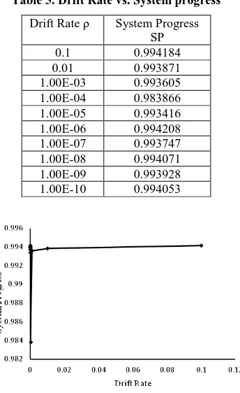
This subsection describes how drift rate affects the system progress. For low value of drift rate the system progress is high little bit .The System Progress of non blocking protocol is not much affected for different values of drift rate the System .Table 5. and Fig.6 illustrates this.
Table 5. Drift Rate vs. System progress
Drift Rate ρ System Progress SP
0.1 0.994184 0.01 0.993871 1.00E-03 0.993605 1.00E-04 0.983866 1.00E-05 0.993416 1.00E-06 0.994208 1.00E-07 0.993747 1.00E-08 0.994071 1.00E-09 0.993928 1.00E-10 0.994053
Fig 7 Drift Rate vs. System Progress
3.2.5
System progress validation
In Table 6. the first column, first entry illustrates that 10 samples of checkpoint interval of length 100 are taken and corresponding System progress of 100,200,…..1000 checkpoint intervals gets evaluated, their average is shown in second column (i.e. 0.99520).The third and fourth column shows their standard deviation, upper and lower confidence limit respectively. Similarly System Progress of other samples
having checkpoint intervals 2000, 3000 …10000 are validated
Similar validation can be applied to other system parameters. The difference between upper and lower confidence limit should be less than 2*Tolerance value. Here tolerance value is 0.001 for 99% confidence
Table 6. System progress validation
Sample No.
System Progress average
σest
Upper Confidence. Limit
4.
CONCLUSION
In this paper the problem of arrival of fault is efficiently discussed. A probabilistic model is developed for evaluation of System progress of the processes along with a particular set of parameters. It is observed that the System Progress is evaluated by introducing the time generated by negative exponential distribution function. The system Progress gets optimizes on particular values of system parameters. A validation regarding the System progress on the basis of set of parameter checkpoint interval length (L) value is derived .Such validation can be evaluated regarding the other set of parameters such as drift rate, fault rate, saved checkpoint time
.
5.
ACKNOWLEDGMENTS
Sincere thanks to HCTM Technical Campus Management Kaithal-136027, Haryana, India for their constant encouragement.
6.
REFERENCES
[1] Chandy K.M. and Lamport L. “Distributed Snapshots:
Determining Global States of Distributed Systems” ACM
Transactions Computer systems vol. 3, no.1. pp. 63-75, Feb.1985
[2] Chaoguang M., Yunlong Z. and Wenbin Y., “A two -phase time-based consistent checkpointing strategy,” in
Proc. ITNG’06 3rd IEEE International Conference on
Information Technology: New Generations, April 10-12, 2006, pp. 518–523.
[3] Chinara Suchistmita and Rath S.K.“An Energy Efficient Mobility Adaptive Distributed Clustering Algorithm for Mobile ad-hoc Network” 978-1-4244-2963-9/08 (2008) IEEE.
[4] Guohong Cao and Singhal Mukesh, “Mutable Checkpoints: a new checkpointing approach for Mobile
Computing Systems”, IEEE Transaction on Parallel and
Distributed Systems, vol. 12, no. 2, pp. 157-172, February 2001
[5] Koo. R. and Toueg. S. “Checkpointing and Rollback
-Recovery for Distributed Systems”. IEEE Transactions on Software Engineering, SE-13(1): pp 23-31, January 1987.
[6] Kumar Lalit, Kumar Awasthi, “A Synchronous Checkpointing Protocol for Mobile Distributed Systems:
Probabilistic Approach” International Journal of Information and Computer Security, Vol.1, No.3 .pp 298-314, 2007.
[7] Lin C., Wang S., and Kuo S., “A Low Overhead
Checkpointing Protocol for Mobile Computing System”
in Proc of the 2002 IEEE Pacific Rim International
Symposium on dependable computing (PRDC’02).
[8] Lin C., Wang S., and Kuo S., “An efficient time-based checkpointing protocol for mobile computing systems
over wide area networks,” in Lecture Notes in Computer
Science 2400, Euro-Par 2002, Springer-Verlag, 2002, pp. 978–982. Also in Mobile Networks and Applications, 2003, vo. 8, no. 6, pp. 687–697.
[9] Neves N., Fuchs W.K., “Using time to improve the
performance of coordinated checkpointing,” In:
Proceedings of 2nd IEEE International Computer Performance and Dependability Symposium, Urbana-Champaign, USA, 1996, pp.282 –291.
[10]Panghal Anil, Panghal Sharda, Rana Mukesh
“Checkpointing Based Rollback Recovery in Distributed Systems” Journal of Current Computer Science and
Technology Vol. 1 Issue 6 [2011]258-266.
[11]Prakash R. and Singhal M., “Low-Cost Checkpointing
and Failure Recovery in Mobile Computing Systems”,
IEEE Transaction on Parallel and Distributed Systems, vol. 7, no. 10, pp. 1035-1048, October1996.
Adaptive Learning for Algorithm Selection in
Classification
Nitin Pise
Research Scholar
Department of Computer Engg. & IT College of Engineering, Pune, India
Parag Kulkarni
Phd, Adjunct Professor Department of Computer Engg. & IT
College of Engineering, Pune, India
ABSTRACT
No learner is generally better than another learner. If a learner performs better than another learner on some learning situations, then the first learner usually performs worse than the second learner on other situations. In other words, no single learning algorithm can perform well and uniformly outperform other algorithms over all learning or data mining tasks. There is an increasing number of algorithms and practices that can be used for the very same application. With the explosion of available learning algorithms, a method for helping user selecting the most appropriate algorithm or combination of algorithms to solve a problem is becoming increasingly important. In this paper we are using meta-learning to relate the performance of machine meta-learning algorithms on the different datasets. The paper concludes by proposing the system which can learn dynamically as per the given data.
General Terms
Machine Learning, Pattern Classification
Keywords
Learning algorithms, Dataset characteristics, algorithm selection
1. INTRODUCTION
The knowledge discovery [3] is an iterative process. The analyst must select the right model for the task he is going to perform, and within it, the right model or algorithm, where the special morphological characteristics of the problem must always be considered. The algorithm is then invoked and its output is evaluated. If the evaluations results are poor, the process is repeated with new selections. A plethora of commercial and prototype systems with a variety of models
and algorithms exist at the analyst’s disposal. However, the selection among them is left to the analyst. The machine learning field has been evolving for a long time and has given us a variety of models and algorithms to perform the classification, e.g. decision trees, neural networks, support vector machines [4], rule inducers, nearest neighbor etc. The analyst must select among them the ones that better match the morphology and the special characteristics of the problem at hand. This selection is one of the most difficult problems since there is no model or algorithm that performs better than all others independently of the particular problem characteristics. A wrong choice of model can have a more severe impact: A hypothesis appropriate for the problem at hand might be ignored because it is not contained in the
model’s search space.
There is an increasing number of algorithms and practices that can be used for the very same application. Extensive research
has been performed to develop appropriate machine learning techniques for different data mining tasks, and has led to a proliferation of different learning algorithms. However, previous work has shown that no learner is generally better than another learner. If a learner performs better than another learner on some learning situations, then the first learner usually performs worse than the second learner on other situations [5]. In other words, no single learning algorithm can perform well compared to the other algorithms and outperform other algorithms over all classification tasks. This has been confirmed by the “no free lunch theorems” [6]. The major reasons are that a learning algorithm has different performances in processing different datasets and that different variety of ‘inductive bias’ [7]. In real-world applications, the users need to select an appropriate learning algorithm according to the classification task that is to be performed [8],[9]. If we select the algorithm inappropriately, it results in a slow convergence or may lead to a sub-optimal local minimum. Meta-learning has been proposed to deal with the issues of algorithm selection [10]. One of the aims of meta-learning is to help or assist the user to determine the most suitable learning algorithm(s) for the problem at hand. The task of meta-learning is to find functions that map datasets to predicted data mining performance (e.g., predictive accuracies, execution time, etc.). To this end meta-learning uses a set of attributes, called meta-attributes, to represent the characteristics of classification tasks, and search for the correlations between these attributes and the performance of learning algorithms. Instead of executing all learning algorithms to obtain the optimal one, meta-learning is performed on the meta-data characterizing the data mining tasks. The effectiveness of meta-learning is largely dependent on the description of tasks (i.e., meta-attributes).
Ensemble methods are learning algorithms that construct a set of classifiers and then classify new data points by taking a vote of their predictions. Combining classifiers or studying methods for constructing good ensembles of classifiers to achieve higher accuracy is an important research topic [1] [2].
The drawback of ensemble learning is that in order for ensemble learning to be computationally efficient, approximation of posterior needs to have a simple factorial structure. This means that most dependence between various parameters cannot be estimated. It is difficult to measure correlation between classifiers from different types of learners. Also there are learning time and memory constraints. Learned concept is difficult to understand.
function. Adaptive learning will be built on the top of ensemble methods.
2. RELATED WORKS
Several algorithm selection systems and strategies have been proposed previously [3][10][11][12]. STATLOG [14] extracts various characteristics from a set of datasets. Then it combines these characteristics with the performance of the algorithms. Rules are generated to guide inducer selection based on the dataset characteristics. This method is based on the morphological similarity between the new dataset and existing collection of datasets. When a new dataset is presented, it compares the characteristics of the new dataset to the collection of the old datasets. This costs a lot of time. Predictive clustering trees for ranking are proposed in [15]. It uses relational descriptions of the tasks. The relative performance of the algorithms on a given dataset is predicted for a given relational dataset description. Results are not very good, with most relative errors over 1.0 which are worse than default prediction. Data Mining Advisor (DMA) [16] is a system that already has a set of algorithms and a collection of training datasets. The performance of the algorithms for every subset in the training datasets is known. When the user presents a new dataset, DMA first finds a similar subset in the training datasets. Then it retrieves information about the performance of algorithms and ranks the algorithms and gives the appropriate recommendation. Our approach is inspired by the above method used in [16].
Most work in this area is aimed at relating properties of data to the effect of learning algorithms, including several large scale studies such as the STATLOG (Michie et al., 1994) and METAL (METAL-consortium, 2003) projects. We will use
this term in a broader sense, referring both to ‘manual’
analysis of learner performance, by querying, and automatic model building, by applying learning algorithms over large collections of meta-data. An instance based learning algorithm (K-nearest neighbor) was used to determine which training datasets are closest to a test dataset based on similarity of features, and then to predict the ranking of each algorithm based on the performance of the neighboring datasets.
3. LEARNING ALGORITHMS AND
DATASET CHARACTERISTICS
In general there are two families of algorithms, the statistical, which are best implemented by an experienced analyst since they require a lot of technical skills and specific assumptions and the data mining tools, which do not require much model specification but they offer little diagnostic tools. Each family has reliable and well-tested algorithms that can be used for prediction. In the case of the classification task [11], the most frequent encountered algorithms are logistic regression (LR), decision tree and decision rules, neural network (NN) and discriminant analysis (DA). In the case of regression, multiple linear regression (MLR), classification & regression trees (CART) and neural networks have been used extensively.
In the classification task the error rate is defined straightforwardly as the percentage of the misclassified cases in the observed versus predicted contingency table. When NNs are used to predict a scalar quantity, the square of the correlation for the predicted outcome with the target response is analogous to the r-square measure of MLR. Therefore the error rate can be defined in the prediction task as:
Error rate = 1 - correlation2 (observed, predicted)
In both tasks, error rate varies from zero to one, with one indicating bad performance of the model and zero the best possible performance.
The dataset characteristics are related with the type of problem. In the case of the classification task the number of classes, the entropy of the classes and the percent of the mode category of the class can be used as useful indicators. The relevant ones for the regression task might be the mean value of the dependent variable, the median, the mode, the standard deviation, skewness and kurtosis. Some database measures include the number of the records, the percent of the original dataset used for training and for testing, the number of missing values and the percent of incomplete records. Also useful information lies on the total number of variables. For the categorical variables of the database, the number of dimensions in homogeneity analysis and the average gain of the first and second Eigen values of homogeneity analysis as well as the average attribute entropy are the corresponding statistics. For the continuous variables, the average mean value, the average 5% trimmed mean, the median, the variance, the standard deviation, the range, the inter-quartile
range, skewness, kurtosis and the Huber’s M-estimator are some of the useful statistics that can be applied to capture the information on the data set.
The determinant of the correlation matrix is an indicator of the interdependency of the attributes on the data set. The average correlation, as it is captured by Crobach-α reliability coefficient, may be still an important statistic. By applying principal component analysis on the numerical variables of the data set, the first and second largest Eigen values can be observed.
If the data set for a classification task has categorical explanatory variables, then the average information gain and the noise to signal ratio are two useful information measures, while the average Goodman and Kruskal tau and the average chi-square significance value are two statistical indicators. Also in the case of continuous explanatory variables, Wilks’ lambda and the canonical correlation of the first discrimination function may be measures for the discriminating power within the data set.
By comparing a numeric with a nominal variable with the
student’s t-test, two important statistics are produced to indicate the degree of their relation, namely Eta squared and the Significance of the F-test.
Table 1. DCT dataset properties [17]
Nr_Attributes Nr_num_attributes Nr_sym_attributes Nr_examples Nr_classes MissingValues_Total MissingValues_relative Mean_Absolute_Skew MStatistic MeanKurtosis NumAttrsWithOutliers MstatDF
MstatChiSq SDRatio
WiksLambda Fract
4. PROPOSED METHOD
Here we are considering properties of scenarios. We need to classify learning scenario. We are extracting features of input data or datasets. We are using the concept of meta-learning. Meta-learning relates algorithms to their area of expertise using specific problem characteristics. The idea of meta-learning is to learn about classifiers or meta-learning algorithms, in terms of the kind of data for which they actually perform well. Using dataset characteristics, which are called meta-features; one predicts the performance results of individual learning algorithms. These features are divided into several categories:
Sample or general features: Here we need to find out the number of classes, the number of attributes, the number of categorical attributes, the number of samples or instances etc.
Statistical features: Here we require to find canonical discriminant, correlations, skew, kurtosis etc.
Information theoretic features: Here we need to extract class entropy, signal to noise ratio etc.
We are proposing adaptive methodology. Different thoughts can be considered, e.g. parameters such as the input data, learning methods, learning policies, learning methods combination. Here there can be a single learner or multiple learners. Also we can use simple voting or averaging while combining the performance of the different learners.
5. EXPERIMENTS
5.1
Experimental Descriptions
Here we need to map the dataset’s characteristics to the performance of the algorithm. We are capturing the
knowledge about the algorithms’ from experiments. Here we are calculating the algorithms’ accuracy on each dataset.
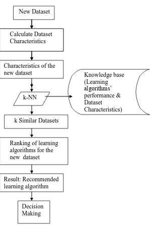
After the experiments, accuracy of each algorithm corresponding to every dataset is saved in the knowledge base for the future use. The Ranking procedure is shown in Figure 1.
Given a new dataset, we use k-NN [7] to find out the most similar dataset in the knowledge base with the new one. K-Nearest Neighbor learning is the most basic instance-based method. The nearest neighbors of an instance are defined in terms of the standard Euclidean distance. Let an arbitrary instance x be described by the feature vector
<a1 (x), a2 (x), --- an(x) >
Where ar (x) denotes the value of the rth attribute of instance x. Then the distance between two instances xi and xj isdefined to be d (xi- xj),
d (xi-xj) = √ (∑(ar (xi) –ar (xj ) )) 2
Here r varies from 1 to n in summation. 24 characteristics are
used to compare the two dataset’s similarities. A distance
function that based on the characteristics of the two datasets is used to find the most similar neighbors, whose performance is expected to be similar or relevant to the new dataset. The recommended ranking of the new dataset is built by
aggregating the learning algorithms’ performance on the similar datasets. The knowledge base KB stores the dataset’s characteristics and the learning algorithms’ performance
k Similar Datasets
Ranking of learning
algorithms for the
new dataset
Result: Recommended
learning algorithm
Decision
Making
New Dataset
Calculate Dataset
Characteristics
Characteristics of the
new dataset
k-NN
Calculate Dataset
Characteristics
Knowledge base
(Learning
algorithms’
performance &
Dataset
Characteristics)
Fig 1: The Ranking of Learning Algorithms
6. RESULTS AND DISCUSSIONS
Here we have used Adult Dataset [13]. The dataset Adult has following features:
48842 instances
14 attributes (6 continuous, 8 nominal)
Contains information on adults such as age, gender, ethnicity, martial status, education, native country, etc.
The instances are classified into either “Salary >50K” or “Salary <= 50K”
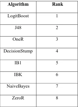
Table 2. Ranking of different algorithms on Adult Dataset
Algorithm Rank
LogitBoost 1
J48 2
OneR 3
DecisionStump 4
IB1 5
IBK 6
NaiveBayes 7
ZeroR 8
Table 3. Correctly & Incorrectly Classified Instances for Adult Dataset
Algorithm % of
Correct classified instances
% of Incorrect classified instances
LogitBoost 84.68 15.32
ZeroR 76.07 23.93
Fig. 2: % Classified instances with top ranked algorithm LogitBoost on Adult Dataset
Figure 2 shows percentage of classified instances with the top ranked algorithm called LogitBoost on Adult Dataset. Here 84.68 % instances are correctly classified.
Figure 3 shows percentage of classified instances with the lowest ranked algorithm called ZeroR on Adult Dataset. Here 76.07 % instances are correctly classified.
Fig. 3: % Classified instances with lowest ranked algorithm ZeroR on Adult Dataset
7. CONCLUSIONS AND FUTURE WORK
In this paper, we present our preliminary work on using meta-learning method for helping user effectively to select the most appropriate learning algorithms and give the ranking recommendation automatically. It will assist both novice and expert users. Ranking system can reduce the searching space, give him/her the recommendation and guide the user to select the most suited algorithms. Thus the system will assist to learn adaptively using the experiences from the past data. In the future work, we will investigate more on our proposed method and test extensively on other datasets. Meta Learning helps improve results over the basic algorithms. Using Meta Characteristics on the Adult dataset to determine an appropriate algorithm, almost 85% correct classification is achieved for LogitBoost algorithm. So out of eight algorithms LogitBoost algorithm is recommended to the user.8. ACKNOWLEDGMENTS
Our thanks to the experts who have contributed towards development of the different algorithms and made them available to the users.
9. REFERENCES
[1] Kuncheva, L, Bezdek J., and Duin, R. 2001 Decision Templates for Multiple Classifier Fusion: An Experimental Comparison, Pattern Recognition. 34, (2), pp.299-314, 2001.
[2] Dietterich, T. 2002 Ensemble Methods in Machine Learning 1st Int. Workshop on Multiple Classifier Systems, in Lecture Notes in Computer Science, F. Roli and J. Kittler, Eds. Vol. 1857, pp.1-15, 2002.
[3] Alexmandros, K. and Melanie, H. J. 2001 Model Selection via Meta-Learning: A Comparative Study. International Journal on Artificial Intelligence Tools. Vol. 10, No. 4 (2001).
[4] Joachims, T. 1998 Text Categorization with Support Vector Machines: Learning with Many Relevant Features. Proceedings of the European Conference on Machine Learning, Springer.
[5]
Schaffer, C. 1994 Cross-validation, stacking and bi- level stacking: Meta-methods for classification learning,In
Cheeseman,
P.
and
Oldford
R.W.(eds)
Selecting
Models from Data: Artificial Intelligence andIV, 51-59.
Correct
Incorrect
[6] Wolpert, D. 1996 The lack of a Priori Distinctions
between Learning Algorithms, Neural Computation, 8, 1996, 1341-1420.
[7] Mitchell, T. 1997 Machine Learning, McGraw Hill.
[8] Brodley, C. E. J.1995 Recursive automatic bias selection for classifier construction, Machine Learning, 20, 63-94.
[9] Schaffer, C. J. 1993 Selecting a Classification Methods by Cross Validation, Machine Learning, 13, 135-143.
[10]Kalousis, A. and Hilario, M. 2000 Model Selection via Meta-learning: a Comparative study, Proceedings of the 12th International IEEE Conference on Tools with AI, Canada, 214-220.
[11]Koliastasis, D. and Despotis, D. J. 2004 Rules for Comparing Predictive Data Mining Algorithms by Error Rate, OPSEARCH, VOL. 41, No. 3.
[12]Fan, L., Lei M. 2006 Reducing Cognitive Overload by Meta-Learning Assisted Algorithm Selection,
Proceedings of the 5th IEEE International Conference on Cognitive Informatics, pp. 120-125, 2006.
[13]Frank, A. and Asuncion, A. 2010. UCI machine learning Repository [http://archive.ics.uci.edu/ml]. Irvine, CA: University of California, School of Information and Computer Science.
[14]Michie, D. and Spicgelhater, D. 1994 Machine Learning, Neural and Statistical Classification. Elis Horwood Series in Artificial Intelligence, 1994.
[15]Todorvoski, L. and Blockeel, H. 2002 Ranking with Predictive Clustering Trees, Efficient Multi-Relational Data Mining, 2002.
[16]Alexandros, K. and Melanie, H. J. 2001 Model Selection
Routing Protocol for Mobile Nodes in Wireless Sensor
Network
Bhagyashri Bansode
Department of Computer Engineering, Pune Institute of Computer Technology, Pune,
Maharashtra, India.
Rajesh Ingle
Phd, Department of Computer Engineering, Pune Institute of Computer Technology, Pune,
Maharashtra, India
ABSTRACT
Wireless sensor network made up of sensor nodes which are fix or mobile. LEACH is clustered based protocol uses time division multiple access. It supports mobile nodes in WSN. Mobile node changes cluster. LEACH wait for two TDMA cycles to update the cluster, within these two cycles mobile
node which changed cluster head, can’t send data to any other
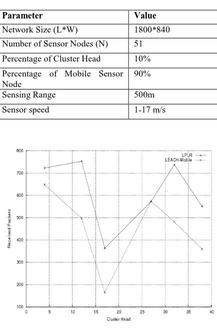
cluster head, it causes packet loss. We propose an adaptive Low Packet Loss Routing protocol which support mobile node with low packet loss. This protocol uses time division multiple access scheduling to reserve the battery of sensor node. We form clusters, each cluster head update cluster after every TDMA cycle to reduce packet loss. The proposed protocol sends data to cluster heads in an efficient manner based on received signal strength. The performance of proposed LPLR protocol is evaluated using NS2.34 on Linux 2.6.23.1.42.fc8 platform. It has been observed that the proposed protocol reduces the packet loss compared to LEACH-Mobile protocol.
Keywords
Cluster based routing, mobility, LEACH-Mobile, WSN
1.INTRODUCTION
A wireless sensor network (WSN) consists of spatially distributed autonomous sensors to monitor physical or environmental conditions, such as temperature, sound, vibration, pressure, humidity, motion or pollutants and to cooperatively pass their data through the network to a main location. Modern networks are bi-directional, also enabling control of sensor activity. The development of wireless sensor networks was motivated by military applications such as battlefield surveillance; today such networks are used in many industrial and consumer applications, such as industrial process monitoring and control, machine health monitoring. WSN consist of mobile or fix sensor nodes. In some cases it consists of hybrid sensor nodes. All nodes sense and send data to server. This increases communication overhead because all nodes are sending data to server. This network containing hundreds or thousands of sensor node and main challenge in WSN is to reduce energy consumption and low packet loss in each sensor node. There are many routing protocols like Destination Sequenced Distance Vector (DSDV), Dynamic Source Routing (DSR), and Ad hoc On Demand Distance Vector (AODV) [1]. These protocols are supported to WSN but they are not suitable for tiny, low capacity sensor nodes and they require high power consumption. Flat-based multi-hop routing protocols, designed for static WSN [2-6], have also been exploited in WSN mobile nodes. However it not supports to mobility of sensor node
The main challenge in WSN is to minimize energy consumption in each sensor node. Many researchers concentrate on the routing protocol that would consume less power and hence prolong network’s life span. Wireless ad hoc network routing protocols have been proposed for routing protocols in WSN.
Low Energy Adaptive Clustering Hierarchy-Mobile (LEACH-Mobile) [7] is routing protocol which support to WSN which have mobile nodes. LEACH-Mobile supports sensor nodes mobility in WSN by adding membership declaration to LEACH protocol. LEACH-Mobile protocol selects heads randomly and form cluster. Cluster head create Time Division Multiple Access (TDMA) schedule. Nodes sense and send that data to cluster head according to TDMA schedule. Mobility of node is big challenge to maintain cluster. Mobile nodes changes cluster continuously. LEACH-Mobile protocol update cluster after every two cycles of TDMA schedule. Packet loss happened in between two cycles of TDMA schedule. Mobile node which is not near to any cluster cannot send data to any cluster head so it causes packet loss.
Sensor nodes in LEACH-Mobile wait for two consecutive failure TDMA cycles, then cluster head decide that it has moved out of its cluster. During these two TDMA cycles sensor node loss the packets. In LPLR, sensor node does not need to wait for two consecutive TDMA cycles from cluster head to make decision. Cluster head directly decides that member node has moved out of its cluster after one TDMA cycle. The data loss is reduced by sending its data to new cluster head and sends join acknowledgment message to the cluster head.
Table 1 Abbreviations
WSN Wireless Sensor Network
DSDV Destination Sequenced Distance Vector
DSR Dynamic Source Routing
AODV Ad hoc On Demand Distance Vector
LEACH-Mobile Low Energy Adaptive Clustering Hierarchy-Mobile
TDMA Time Division Multiple Access
LPLR Low Packet Loss Routing CSMA Carrier Sense Multiple Access
CA MAC Collision Avoidance Medium Access Control
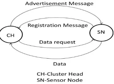
CH Cluster Head
SN Sensor Node
2.
LOW PACKET LOSS ROUTING
Low Packet Loss Routing (LPLR) is Low Packet Loss Routing protocol for wireless sensor network. LPLR proposes to handle packet loss and efficiently use energy resources. In this protocol, cluster head receives the data not only from its members during TDMA allocated time slot but also from other lost sensor nodes. WSN consist of mobile and fix both type of nodes. After cluster formation mobile node can change cluster. LPLR gives entry to mobile node in new cluster and TDMA schedule to send data.
2.1
Selection of Cluster Head
Protocols like TEEN [8] and APTEEN [9] used stationary but dynamically changing cluster head. In some protocol where sensor nodes are mobile cluster head is selected according to mobility factor [10]. The node with the smallest mobility factor in each cluster is chosen as cluster head. In LEACH-Mobile cluster head assumed to be stationary and static in order to control mobility. In proposed protocol we elect cluster heads randomly. It assumed to be stationary and static through the rounds.
2.2
Formation of Cluster
After a cluster head has been selected, it broadcasts an advertisement messages to the rest of the sensor nodes in the network as in LEACH and LEACH-Mobile. For these advertisement messages, cluster heads use a Carrier Sense Multiple Access with Collision Avoidance Medium Access Control (CSMA/CA MAC) protocol. All cluster heads use the same transmit energy when transmitting advertisement
messages. Sensor nodes must keep their receivers “ON” in
order to receive the advertisement message from their cluster head. After sensor nodes have received advertisement messages from one or more cluster heads, sensor nodes compare the received signal strength for received advertisement messages, and decide the cluster to which it will belong. By assuming symmetric propagation channels, the sensor node selects cluster head to which the minimum amount of transmitted energy is needed for communication. In the case of a tie, a random cluster-head is chosen. After deciding the cluster it will belong, the node sends registration message to inform the cluster head. This advertisement messages are transmitted to the cluster heads using CSMA/CA MAC protocol. During this phase, all cluster heads must keep their receiver on.
2.3
TDMA Schedule Creation
After cluster head receives registration messages from the nodes that would like to join the cluster, the cluster head creates a TDMA schedule based on the number of nodes and assigns each node a time slot to transmit the data. This schedule is broadcasted to all the sensor nodes in the cluster. All sensor nodes will transmit data according to TDMA schedule
2.4
Data Transmission
Once the clusters are created and the TDMA schedule is fixed, data transmission from sensor nodes to their cluster heads begin according to their TDMA scheduled. Upon receiving data request from the cluster head the sensor node switches on its radio transmitter, adjusts transmission power and sends its data. At the end of the transmission, the node turns off its radio, thus we can save the battery of sensor node. The cluster head must keep its radio on to send data request messages, receive data from the sensor nodes and to send and receive other messages needed to maintain the network. Sensor node receives data request message from the cluster head, it will send its data back to the cluster head. If the sensor nodes did not receive data request message from its cluster head, it will send the message to a free cluster head.
3.
LPLR ALGORITHM
Cluster Head – CH1 to CH6 Sensor node – S1 to S51 1. Select head randomly.
Select cluster head CH1 to CH6 from S1 to S51 sensor node. 2. All cluster head broadcast advertisement message, from S1 to S51 except cluster heads.
3. Sensor node receives advertisement messages from CH1 to CH6.
4. Compare received signal strength. Select maximum received signal strength. According to that received signal strength sensor node select head CH1 to CH6.
5. Sensor node sends registration message to cluster head. 6. Cluster head create TDMA schedule and broadcast to all member nodes.
7. According to TDMA schedule cluster head sends data request message to member node.
8. Member node sends data to cluster head
.
Figure 1: Messages of Cluster Head and Sensor Node
3.1
Cluster Head
and broadcast that schedule. When cluster head finishes receiving data messages from all sensor nodes, it will check whether it receives data messages from all members. Any of the member nodes did not send the data message then cluster head remove that sensor node from cluster. Cluster head again broadcast advertisement message to all nodes and update the cluster. Updating of cluster causes entry of new mobile nodes in TDMA schedule of cluster.Figure1 shows messages transfers and receives by cluster head.
3.2
Sensor Node
Sensor node receives advertisement message from one or more cluster head. According to received signal strength node select head. Node send registration message to selected head and get entry into TDMA schedule of that cluster. Member node sends data to cluster head according to TDMA schedule when it receive data request message from cluster head. If sensor node does not receive any advertisement or any data request message then it sends data to free cluster head. Figure1 shows messages transfers and receives by sensor node.
4.
SIMULATION RESULT
We have simulated LPLR and LEACH-Mobile using NS2.34 on Linux 2.2.23.1.42.fc8 platform with parameters as shown in Table 1. Basic hardware requirement for this simulation is pentium4 processor, 512mb RAM, 10GB hard disk.
Table 2 Performance Parameter
Parameter Value
Network Size (L*W) 1800*840 Number of Sensor Nodes (N) 51 Percentage of Cluster Head 10%
Percentage of Mobile Sensor Node
90%
Sensing Range 500m
Sensor speed 1-17 m/s
Figure2. Total Number of Received Packets
Figure2. shows total number of packets received by cluster head from member node. We applied LEACH-Mobile to network and observed number of packets received by each
cluster head from member node in the WSN. We applied LPLR to the same WSN and observed same result. We can see from figure2 the LPLR achieves significant improvement compared to LEACH-Mobile. We can conclude that packet loss decreasesusing LPLR
Figure3. Remaining Energy of Nodes
Figure3 shows remaining energy of every sensor node in the WSN. Member node wakes up to send the data according to TDMA schedule otherwise they are in sleep mode so we can reduce energy consumption. We can compare the remaining energy of sensor node in LEACH-Mobile and LPLR from figure3. We can say that sensor node can reserve more battery using LPLR than LEACH-Mobiles.
Figure4. Packet Delivery Ratio
Figure4 shows packet delivery ration of cluster head of LPLR and LEACH-Mobile. From this figure we can compare delivery ratio of both protocol and performance of LPLR is efficient than LEACH-Mobile.
5.
CONCLUSION
are working on cluster head failure case to get better result than proposed LPLR protocol.
We proposed efficient routing protocol for mobile nodes in wireless sensor network. LPLR protocol is efficient in energy consumption and packet delivery in the network. It forms cluster. Cluster head create and maintain TDMA schedule. Sensor node wake up at the time of sending data and it goes into sleep mode, it reserve the battery of sensor node. Important feature of this protocol is it update cluster after every TDMA cycle. So every mobile node can get entry into new cluster and can send data. LPLR also maintain a free cluster head. Mobile sensor node which is not in the range of any cluster or node which are moved from one cluster and waiting for new cluster they sends data to free cluster head. It reduces packet loss. We have simulated LEACH-Mobile and proposed LPLR protocol and got efficient result of LPLR.
6.
REFFERENCES
[1] C.Perkins and P.Bhagwat. "Highly Dynamic Destination-Sequenced Distance-Vector Routing (DSDV) for Mobile Computers," presented at the ACM '94 Conference on Communications Architectures, Protocols and Applications, 1994.
[2]W. Heinzelman, J. Kulik, and H. Balakrishnan, "Adaptive protocols for information dissemination in wireless sensor networks," Proc. 5th ACM/IEEE Mobicom Conference (MobiCom '99), Seattle, WA, August, 1999, pp. 174-85.
[3]J.Kulik, W. R. Heinzelman, and H. Balakrishnan, "Negotiation-based protocols for disseminating information in wireless sensor networks," Wireless Networks, Vol. 8, 2002, pp. 169-185.
[4] C. Intanagonwiwat, R. Govindan, and D. Estrin, "Directed diffusion: a scalable and robust communication paradigm for sensor networks," Proc. of ACM MobiCom '00, Boston, MA, 2000, pp. 56-67.
[5] D. Braginsky and D. Estrin, "Rumor routing algorithm for sensor networks," Proc. of the 1st Workshop on Sensor Networks and Applications (WSNA), Atlanta, GA, October 2002.
[6]Y. Yao and J. Gehrke, "The cougar approach to in-network query processing in sensor networks", in SIGMOD Record, September 2002.
[7]Guofeng Hou, K. Wendy Tang, "Evaluation of LEACH
protocol Subject to Different Traffic Models,” presented
at the first International conference on Next Generation Network (NGNCON 2006), Hyatt Regency Jeju, Korea/July 9-13,1006
[8]A. Manjeshwar and D. P. Agarwal, "TEEN: a routing protocol for enhanced efficiency in wireless sensor networks," presented at the 1st Int. Workshop on Parallel and Distributed Computing Issues in Wireless Networks and Mobile Computing, April 2001.
[9]A. Manjeshwar and D. P. Agarwal, "APTEEN: A hybrid protocol for efficient routing and comprehensive information retrieval in wireless sensor networks," Parallel and Distributed Processing Symposium., IPDPS 2002, pp. 195-202.
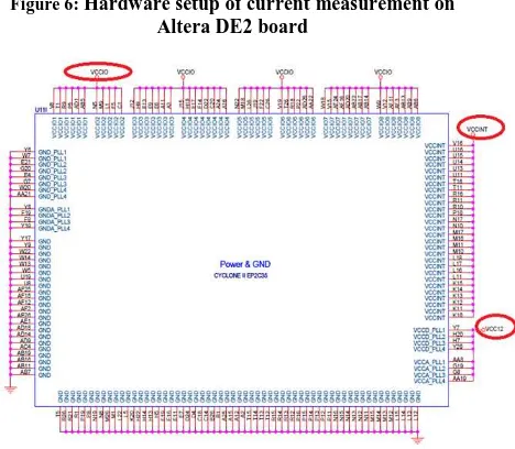
32-Bit NxN Matrix Multiplication: Performance Evaluation
for Altera FPGA, i5 Clarkdale, and Atom Pineview-D Intel
General Purpose Processors
Izzeldin Ibrahim Mohd
Faculty of Elect. Engineering, Universiti Teknologi Malaysia,
81310 JB, Johor
Chay Chin Fatt
Intel Technology Sdn. B