in PROBABILITY
VARIABLY SKEWED BROWNIAN MOTION
MARTIN BARLOW1
University of British Columbia Vancouver, BC V6T 1Z2, CANADA email: [email protected]
KRZYSZTOF BURDZY2
University of Washington Seattle, WA 98195-4350, U.S.A. email: [email protected]
HAYA KASPI3
Technion Institute Haifa, 32000, ISRAEL
email: [email protected]
AVI MANDELBAUM3
Technion Institute Haifa, 32000, ISRAEL
email: [email protected]
submitted September 15, 1999Final version accepted March 1, 2000 AMS 1991 Subject classification: 60J65, 60H10
Skew Brownian motion, Brownian motion, stochastic differential equation, local time
Abstract
Given a standard Brownian motionB, we show that the equation Xt=x0+Bt+β(LXt ), t≥0 ,
has a unique strong solution X. Here LX is the symmetric local time of X at 0, and β is a
given differentiable function with β(0) = 0,−1 < β′(·)<1. (For linear β(·), the solution is the familiar skew Brownian motion).
1
Introduction
In this paper we consider the following stochastic differential equation:
Xt=x0+Bt+β(LXt ), t≥0. (1.1)
1
Research partially supported by an NSERC (Canada) grant.
2
Research partially supported by NSF grant DMS-9700721.
3
Research partially supported by the Fund for the Promotion of Research at the Technion.
HereB={Bt, t≥0}is a standard Brownian motion on a filtered probability space (Ω,F,(Ft), P),
andβ is a (fixed) differentiable function, which satisfiesβ(0) = 0,−1< β′(x)<1. We seek a solution pair (X, LX) to (1.1) where
X ={Xt, t≥0}is a continuous semimartingale, adapted
to (Ft) andLX={LXt , t≥0} is the symmetric local time ofX at 0.
The special case β(x) =β0x was introduced by Harrison and Shepp [HS], who proved that
the unique strong solution to (1.1) is skew Brownian motion (see Itˆo and McKean [IM], Walsh [W1]). Note that the extreme cases β′ ≡ +1 and β′ ≡ −1 give rise to reflected Brownian
motion.
A related stochastic differential equation, introduced by Weinryb [We], is
Xt=x0+Bt+
Z t
0
α(s)dLb0s, t≥0,
whereαis a given deterministic function andLb0 is here the nonsymmetric local time ofX at
0. In [We] it was shown that a unique strong solution exists if|α| ≤ 12.
Our motivation for studying equation (1.1) arose from continuous-time multi-armed bandits – see [KM1, KM2, M]. Let ϕbe a monotone strictly increasing function withϕ(0) = 0. Given two independent one-dimensional Brownian motionsW1andW2, consider the multi-parameter
time change Zi(t) =Wi(Ti(t)), where T1(t) +T2(t) = t, t ≥0, and the processes Ti(t) are
chosen so that T1(·) increases only at times t when ϕ(W1(T1(t))) > W2(T2(t)), while T2(·)
increases if the reversed inequality applies.
Multi-parameter time changes of this kind are calledstrategiesin the context of multi-armed bandits, andoptional increasing paths[W2] in the theory of multi-parameter processes. (The pair (T1(t), T2(t)) allocates play between the two ‘bandits’W1 andW2.)
To see the relation between this and (1.1), assume for simplicity thatx0= 0 and consider the
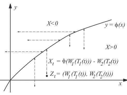
time-changed process Z= (Z1, Z2) as a stochastic process in the plane (see Figure 1). When
the process Z is above the curve C = {(x1, x2) | x2 = ϕ(x1)}, then only T1 is increasing,
and soZ moves horizontally. SimilarlyZ moves vertically belowC. The motion onC is not quite so obvious, but it turns out thatZ crawls upwards alongCat the local time rate, while performing excursions away from it.
Let X be the distance from Z to the curve C, in the following sense. When Z is above the curve the distance is measured horizontally, and given a negative sign; otherwise, the distance is measured vertically and given a positive sign. Then, working on the filtration generated by Z, we prove in Section 2 that X is a solution to (1.1). This proves weak existence for the equation (1.1): weak because both the ‘solution’X and the driving processB are constructed from the pair (W1, W2).
For those readers that are not familiar with the theory of multi armed bandits and multi parameter time changes, we provide another weak solution, which follows along the lines of the construction in [W1] of linearly skewed Brownian motion. We would like to thank the referee for pointing out that this construction can be carried easily to our situation.
In Section 3, we prove pathwise uniqueness of the solution to (1.1). We will show there that any two solutions yield a third solution whose local time at zero dominates the local times of both original solutions. This leads to pathwise uniqueness, using the fact thatLX corresponding to
any solution to (1.1) must be the local time of a reflected Brownian motion. Weak existence, combined with pathwise uniqueness, establishes existence and uniqueness of a strong solution to (1.1), via the classical result of Yamada and Watanabe.
Recall from [RY], Chapter VI, the definition of the non-symmetric local times Lbat of a
y = (x)
φ
1 2 2
X = (W (T (t))) - W (T (t))
φ
1 t
y
x
X<0
X>0
Z = (W (T (t)), W (T (t)))
1 1 2 2
t
Figure 1: The processZ moves horizontally(vertically) above(below) the curvey=ϕ(x).
by
LXt =
1 2(Lb
0
t+Lb0t−),
and satisfies the following version of Tanaka’s formula:
|Xt|=|X0|+
Z t
0 g
sgn (Xs)dXs+LXt ,
where
g sgnx=
−1 ifx <0, 0 ifx= 0, 1 ifx >0 .
2
A Weak Solution
We begin with a lemma concerning the solutions to (1.1).
Lemma 2.1 (a) Let(X, L)satisfy
Xt=x0+Bt+β(Lt), t≥0,
and suppose that Lis a process of locally finite variation with1(Xs6=0)dLs= 0. Then|Xt|is a reflecting Brownian motion.
(b) The processes Lb0,Lb0− andLX are related by:
b L0t=LX
t +β(Lt), Lbt0−=LXt −β(Lt).
Proof. (a) Apply the symmetric version of Tanaka’s formula toX:
|Xt|=|x0|+
Z t
0 g
As gsgn (0) = 0 and 1(Xs6=0)dLs= 0,
SinceX andB differ by a process of finite variation Z t
so that the stochastic integral in (2.1) is a Brownian motion,V say. Hence (see [RY], Exercise VI.1.16), L|tX|=−infs≤tVs, so we can write
|Xt|=|x0|+Vt−inf s≤tVs.
This implies that |X|is a reflected Brownian motion. (b) By [RY], Theorem VI.1.7,
b
We now construct two weak solutions to (1.1). The first one is straight forward and is close in nature to Walsh’s construction of (linearly) skewed Brownian motion in [W1], the second, as described in the introduction, arises from multi armed bandits. Since it is trivial to construct a solution to (1.1) up to the time of the first hit byX of 0, in what follows we takex0= 0.
Given β we wish to construct a functionϕsuch that
ify =ϕ(u) +u thenβ(y) =ϕ(u)−u. (2.2)
This is easy to do: let y(u) be the unique realy such that u=12(y−β(y) – unique since the functiony−β(y) is strictly increasing. Now define
ϕ(u) = 1
time change associated with the increasing process
At= 4
Z t
0
That is
Proposition 2.2 Xtβ satisfies (1.1)
Proof
By [RY] Proposition VI (4.3)
rβ(Bt, L0t) = 2
Our second weak solution originates from the theory of multi armed bandits, and since this was our motivation to study the problem we shall describe it briefly. The framework is that of general multi-armed bandits, but here we introduce only concepts that are directly relevant to our problem. The complete set-up can be found in [KM1],[KM2], or [M].
Let (W1(t)) and (W2(t)) be two independent Brownian motions started at 0. Let (Ft1) and
(F2
t) be their respective filtrations, completed and right-continuous as usual. Set S = IR2+,
and introduce the multi-parameter filtration (Fs), given by
We look for a strategyT(t) = (T1(t), T2(t)) that does the following:
T1(t) increases at rate 1 if ϕ(W1(T1(t))< W2(T2(t)), and
T2(t) increases at rate 1 if ϕ(W1(T1(t)))> W2(T2(t)).
The existence of such a strategy follows for example from [M]. We also have from there that this strategy is unique – but we will not need this. Here is an outline of the construction. Define
D={(s1, s2)∈S :ϕ( sup u1≤s1
W1(s1))> sup u2≤s2
W2(s2)}.
It is clear that the closureD ofD has the following three properties:
(i) {(s1,0) :s1≥0} ∈D,
(ii) (s1, s2)∈D⇒ {(u1, u2) :u1≥s1, 0≤u2≤s2} ∈D,
(iii) {s∈D} ∈ Fs.
By Theorem 2.7 of [W2], the northwest boundary of D can be parametrized as a strategy T = (T1, T2), with respect to the filtration (Fs), which is the one we are seeking: T1 increases
at rate 1 when
W2(T2(t))> ϕ(W1(T1(t)),
and T2 increases at rate 1 when W2(T2(t)) < ϕ(W1(T1(t)). (In the language of [M], such a
strategyfollows the leader betweenϕ(W1)andW2).
With the strategy T as above, defineGt=FT(t), and let
Z1(t) =W1(T1(t)), Z2(t) =W2(T2(t)), t≥0, (2.9)
Bt=Z1(t)−Z2(t), t≥0. (2.10)
It is clear thatZiand (Zi)2−Tiare continous (Gt) martingales, so thathZiit=Ti(t). Therefore
(Bt) is a (Gt) Brownian motion, since it is a continuous martingale with quadratic variation
hBit=T1(t) +T2(t) =t.
WriteZi+(t) = sups≤tZi(s). AsT(t) is on the boundary ofDwe must have
ϕ(Z1+(t)) =Z2+(t).
WriteUt=Z1+(t); if Ztis not on the curveC={(x, y) :y=ϕ(x)}, then it will return toC
at the point (Ut, ϕ(Ut)). So
Ut=Z1(t)∨ϕ−1(Z2(t)). (2.11)
Note thatU is constant on each excursion ofZaway from the curveC, and thatUis increasing. The signed horizontal/vertical distance of (Z1, Z2) from the curveC is given by
Xt= (ϕ(Ut)−Z2(t))−(Ut−Z1(t)). (2.12)
andXt|the horizontal/vertical distance of (Z1, Z2) from Cis given by
|Xt|=ϕ(Ut)−Z2(t) +U(t)−Z1(t). (2.13)
Define
Lt=ϕ(Ut) +Ut. (2.14)
Note that all these processes are semimartingales (with respect to (Gt)), and thatLis increasing
Theorem 2.3 The pair (X, L), given by (2.12)–(2.14) solves equation (1.1):
Xt=Bt+β(Lt), t≥0, (2.15)
and(Lt)is the symmetric local time of (Xt)at0.
Proof. Using (2.2 ) we have from (2.14) that
β(Lt) =ϕ(Ut)−Ut.
So by (2.10)
Bt+β(Lt) =Z1(t)−Z2(t) +ϕ(Ut)−Ut=Xt,
proving that the pair (X, L) satisfies the equation (2.15).
Further, arguing as for Bt above, ˜Bt =−W1(T1(t))−W2(T2(t)) is a Brownian motion with
respect to (Gt) and
|Xt|= ˜Bt+Lt. (2.16)
Our result will follow from the Tanaka formula once we note that
˜
Bt=−(Z1(t) +Z2(t)) =−
Z t
0 g
sgn (Xs)dBs=−
Z t
0 g
sgn (Xs)dXs. (2.17)
Remark 2.4 Note that for the second weak solution it is enough to require thatβ is differ-entiable, rather thanC1as is required for the first weak solution.
3
Strong Uniqueness
Theorem 3.1 There exists a unique strong solution to (1.1). The proof of Theorem 3.1 uses the following lemma.
Lemma 3.2 Let X be a continuous semimartingale, let A be of integrable variation and let Y =X+A. Then
1(As=0)dL
X
s = 1(As=0)dL
Y s.
Remark 3.3 The statement above with random measures is equivalent to saying that for any bounded previsible H
Z t
0
Hs1(As=0)dL
X s =
Z t
0
Hs1(As=0)dL
Y s.
Proof of Lemma 3.2. Suppose first thatAt≥0 for all t. Then Y ∨X =Y, and so, since
Y −X =Ahas zero local time, by Exercise (1.21)(c) of [RY]
dbL0s(Y) = 1(Xs<0)dbL
0
s(Y) + 1(Ys≤0)dbL
0 s(X).
Hence sinceAs= 0 andYs= 0 impliesXs= 0, we have
1(As=0)dbL
0
s(Y) = 1(As=0)dbL
If A is not non-negative, let A =A+−A−, whereA+ =A∨0, A− = (−A)∨0. Then set
L0(−X) it also holds for the left local timesLb0−, and so, by addition, for the symmetric local timesLX andLY.
Proof of Theorem 3.1. To prove pathwise uniqueness, assume that there exist two strong solutions (X1
t) and (Xt2) to (1.1), and let (L1t), (L2t) be their respective symmetric continuous
local times. Define a new process (Yt) by
Yt=x0+Bt+β(L1t∨L Note thatAis of integrable variation. Therefore by Lemma 3.2
1(As=0)dL
InterchangingX1 andX2, and multiplying by the previsible process 1 (L2
all reflected Brownian motions. ThusLY
t =L1t∨L2t,L1t andL2t are all local times of reflected
Brownian motions, and so all have the same distribution. SoEL1t =EL2t =EL1t∨L2t, which
implies thatL1t=L2tfor allt, a.s. This in turn implies thatXt1=Xt2for allt, so that pathwise
uniqueness holds for (1.1).
Remark 3.4 Uniqueness in law of the solution to (1.1) is also part of the Yamada- Watanabe result. It may also be derived independently, as in [We], by noting that if (Xt) solves (1.1)
andgt(λ) =E(eiλXt), thengt(λ) satisfies
gt(λ) =eiλx0−
λ2
2 Z
gs(λ)ds+iλh(t),
where h(t) = E(β(Lt)) and (Lt) is the symmetric local time of reflected Brownian motion
started atx0.
Remark 3.5 While Theorem 3.1 proves that the solution X of (1.1) is FB adapted, and
so a functional of the driving Brownian motion B, it does not give any procedure for the construction ofX fromB. We may compare this with the case of reflecting Brownian motion (i.e. β(x) =x), where (ifx0= 0) then Xt=Bt−infs≤tBs.
However, it is a general principle in the theory of stochastic differential equations that if path-wise uniqueness holds, then any ‘reasonable’ approximation scheme will converge in probability to the solutionX. See Jacod and Memin [JM], Kurtz and Protter [KP]. The argument outlined below comes from Lemma 5.5 of [KP].
SupposeXn
t =Fn(B, t) are (adapted) functionals of B such that{(Xn, B), n≥1} is tight in
the Skorohod topology, and any weak limit point (X′, B) gives a solution X′ to (1.1). Then
this also applies to{(Xn, B, Xm, B), n≥1, m≥1}. If (X′, B, X′′, B) is a weak limit point,
then asX′andX′′are both solutions of (1.1), we haveX′=X′′. HenceXn−Xmconverges in
law to 0, and so (Xn) is a Cauchy sequence in probability. Thus (Xn) converges in probability
to a solution of (1.1).
References
[HS] Harrison, J.M. and Shepp, L.A. (1981), On skew Brownian motion,Ann. Probab. 9(2), 309–313.
[IM] Itˆo, K. and McKean, H.P. (1965),Diffusion Processes and Their Sample Paths, Springer, New York.
[KM1] Kaspi, H. and Mandelbaum, A. (1995), L´evy bandits: Multi- armed bandits driven by L´evy processes,Ann. Probab. 5(2), 541–565.
[KM2] Kaspi, H. and Mandelbaum, A. (1997), Multi-armed bandits in discrete and continuous time. To appear inAnn. Appl. Probab.
[KP] Kurtz, T.G. and Protter, P. (1991), Weak limit theorems for stochastic integrals and stochastic differential equations. Ann. Probab. 19(3), 1035-1070.
[JM] Jacod, J. and Memin J. (1981), Weak and strong solutions of stochastic differential equations: Existence and stability, Stochastic Analysis, Lecture Notes in Mathematics 851, 169-212, Springer, Berlin.
[M] Mandelbaum, A. (1987), Continuous multi-armed bandits and multiparameter processes, Ann. Probab. 15, 1527–1556.
[W1] Walsh, J.B. (1978), A diffusion with discontinuous local time,Temps Locaux Asterisque, 52–53, 37–45.
[W2] Walsh, J.B. (1981), Optional increasing paths, Colloque ENST- CNET, Lecture Notes in Math. 863, 172–201, Springer, Berlin.