El e c t ro n ic
Jo ur n
a l o
f P
r o b
a b i l i t y Vol. 12 (2007), Paper no. 9, pages 229–261.
Journal URL
http://www.math.washington.edu/~ejpecp/
Asymptotics of Bernoulli random walks, bridges,
excursions and meanders with a given number of
peaks
Jean-Maxime Labarbe Universit´e de Versailles 45 avenue des Etats-Unis
78035 Versailles cedex [email protected]
Jean-Fran¸cois Marckert CNRS, LaBRI Universit´e Bordeaux 1 351 cours de la Lib´eration
33405 Talence cedex [email protected]
Abstract
A Bernoulli random walk is a random trajectory starting from 0 and having i.i.d. incre-ments, each of them being +1 or−1, equally likely. The other families quoted in the title are Bernoulli random walks under various conditions. A peak in a trajectory is a local maximum. In this paper, we condition the families of trajectories to have a given number of peaks. We show that, asymptotically, the main effect of setting the number of peaks is to change the order of magnitude of the trajectories. The counting process of the peaks, that encodes the repartition of the peaks in the trajectories, is also studied. It is shown that suitably nor-malized, it converges to a Brownian bridge which is independent of the limiting trajectory. Applications in terms of plane trees and parallelogram polyominoes are provided, as well as an application to the “comparison” between runs and Kolmogorov-Smirnov statistics.
AMS 2000 Subject Classification: Primary 60J65, 60B10.
1
Introduction
Let N ={0,1,2,3, . . .} be the set of non-negative integers. For any n ∈ N, we denote by Wn
the set of Bernoulli chains with nsteps :
Wn={S= (S(i))0≤i≤n :S(0) = 0, S(i+ 1) =S(i)±1 for any i∈J0, n−1K}.
The sets of Bernoulli bridgesBn, Bernoulli excursionsEn, Bernoulli meandersMnwithn steps
are defined by
Bn = {S :S∈ Wn, S(n) = 0},
En = {S :S∈ Wn, S(n) = 0, S(i) ≥0 for anyi∈J0, nK},
Mn = {S :S∈ Wn, S(i)≥0 for any i∈J0, nK}.
The cardinalities of these sets are given by
#Wn= 2n, #B2n=
proved for instance thanks to the cyclical lemma (see also the 66 examples of the appearance of the Catalan numbers #E2n in combinatorics in Stanley (23, ex. 6.19 p.219)), and the last one,
may be proved iteratively or thanks to a bijection with Bernoulli bridges (see Section 4.4).
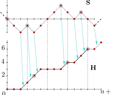
Letn∈N. For everyS∈ Wn, the set of peaks of S, denoted by S∧, is defined by
S∧ ={x :x∈J1, n−1K, S(x−1) =S(x+ 1) =S(x)−1}.
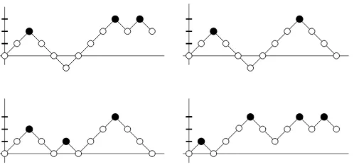
Figure 1: Trajectories fromW12(3),B (2) 12,E
(3)
12 , andM (4)
12. Black dots correspond to peaks.
The formula giving #E2n(k) is due to Narayana (18) computed in relation with pairs of
k-compositions ofnsatisfying some constraints (see also Stanley (23, ex. 6.36 p.237) and Theorem 3.4.3 in Krattenthaler (14), with µ = 1, e1 =e2 = n). The formula giving #B(k)2n can be also
found in (14, Formula (3.6)). The survey (14) of Krattenthaler is very related to the present work and we refer the interested reader to this work and references therein. Among other things, he investigates the link between the number of peaks in some Bernoulli trajectories and the tra-jectories themselves (14, Theorem 3.4.4) (see also Section 1.3). His results concern also the enumerations of trajectories with a prescribed number of peaks staying above a given line, as well as some multidimensional case (the number of non intersecting Bernoulli trajectories with a total number of turns).
LetPwn,Pbn,Pen andPnm be the uniform law onWn,Bn,En, and Mn andP
w,(k)
n ,P
b,(k)
n ,P
e,(k)
n and Pmn,(k) be the uniform law onWn(k),Bn(k),En(k) andM(k)n . Forx∈ {w,b,e,m}, a random variable
under Pxn,(k) is then simply a random variable under Px
n conditioned to have k peaks. We are
interested in the asymptotic behavior of random chains under the distributionsPxn,(k), when n
and k=Kn go to infinity.
LetC[0,1] be the set of continuous functions defined on [0,1] with real values. For anyS∈ Wn,
denote un the function inC[0,1] obtained fromS by the following rescaling:
un(t) =
1
√
n S(⌊nt⌋) +{nt}(S(⌈nt⌉)−S(⌊nt⌋))
for anyt∈[0,1]. (2)
We call Brownian bridge b, Brownian excursion e and Brownian meander m the (normalized) processes characterized as follows : let w be a 1-dimensional standard Brownian motion. Let d= inf{t :t ≥1,wt = 0} and g = sup{t :t ≤1,wt = 0}. Almost surely, we haved−g >0,
g∈(0,1). The processes b,e and mhave the following representations :
(bt)t∈[0,1] (d)
= w√gt g
t∈[0,1], (et)t∈[0,1] (d)
= |w√d+(g−d)t|
d−g
t∈[0,1], (mt)t∈[0,1] (d)
= |w√(1−g)t|
1−g
t∈[0,1].
Theorem 2. For any x∈ {w,b,e,m}, under Px
n, un (d)
−−→
n x in C[0,1]endowed with the topology
of the uniform convergence.
In the casex∈ {b,e}, even if not specified, it is understood thatn→+∞ in 2N.
In fact, Theorem 2 can be proved directly, thanks to the elementary enumeration of paths passing via some prescribed positions in the model of Bernoulli paths. The method used to show the tightnesses in our Theorem 4 may be used to prove the tightness in Theorem 2; thanks to some probability tricks, this reduces to show the tightness underPw
n, which is simple.
The finite dimensional distributions of w,e,b and m are recalled in Section 3.1. Numerous relations exist between these processes, and their trajectories, and a lot of parameters have been computed. We refer to Bertoin & Pitman (4), Biane & Yor (5), Pitman (20) to have an overview of the subject. These convergences have also provided some discrete approaches to the computation of values attached to these Brownian processes, and the literature about that is considerable, see e.g. Cs´aki & Y. Hu (7), and references therein.
We introduce the counting process of the number of peaks : for anyS∈ Wn, denote by Λ(S) =
(Λl(S))l∈J0,nK the process :
Λl(S) = #S∧∩J0, lKfor anyl∈J0, nK. (3)
ForS∈ Wn, Λn(S) = #S∧ is simply the total number of peaks inS. We have
Proposition 3. For any x∈ {w,b,e,m}, under Pxn,
Λn−n/4
√
n
(d)
−−→
n N(0,1/16),
where N(0,1/16) denotes the centered Gaussian distribution with variance 1/16.
We will now describe the main result of this paper. Its aim is to describe the influence of the number of peaks on the shape of the families of trajectories introduced above. We will then condition the different families by #S∧ =Knfor a general sequence (Kn) satisfying the following
constraints :
(H) =For any n, Kn∈N, lim
n Kn= +∞, limn n/2− Kn= +∞
.
Notice that for everyS ∈ Wn, #S∧ ∈ J0,⌊n/2⌋K and then (H) is as large as possible to avoid
that the sequences Kn and n/2− Kn have a finite accumulation point.
We setpn:= 2Kn/nand
βn:= p
n(1−pn)/pn, andγn:= p
Each peak can be viewed to be made by two consecutive steps; hence, if you pick at random one step of a trajectory underPx,(Kn)
n , the probability that this step belongs to a peak ispn.
We considerSand Λ(S) as two continuous processes on [0, n], the values between integer points being defined by linear interpolation. The normalized versions of S and Λ(S) are respectively denoted bysn and λn :
wherebbis a Brownian bridge independent ofxand where the weak convergence holds inC([0,1])2 endowed with the topology of uniform convergence.
Hence, under Px,(Kn)
n , up to the scaling constant, the process sn behaves as under Pnx. The
normalizing factorβn, that will be explained later in the paper, indicates the order of magnitude
of the processS underPx,(Kn)
n (βnis a decreasing function ofKn). The normalizing constantγn
is smaller than pn/4 whatever is pn; γn gives the asymptotic order of the “linearity defect” of
t7→Λnt. The fact that (λn) converges to a Brownian bridge independent of the limit trajectory
is quite puzzling. For example, under Pne, one would expect that only few peaks appear in a neighborhood of 0, this resulting in a negative bias in λn near 0. This must be true, but this
bias is not important enough to change the asymptotic behavior ofλn.
A second direct corollary of Theorem 4 is stated below:
Corollary 5. For any x∈ {w,b,e,m}, under Pnx, we have
where wb is a Brownian motion independent of x,bb is a Brownian bridge independent of xand where the weak convergences hold inC([0,1])2 endowed with the topology of uniform convergence.
Theorem 2 is of course a consequence of Corollary 5.
By Proposition 3 and Theorem 4, underPx
n, the five-tuple
4Λn√−n/4
n ,
S(nt) ˜ βn
t∈[0,1]
,2
Λnt−tΛn
˜ γn
t∈[0,1]
,2√γ˜n
n, ˜ βn
√
n
!
converges in distribution to
(N,(st)t∈[0,1],(λt)t∈[0,1], A, B)
where N is a centered Gaussian random variable with variance 1 and where conditionally on N, (s, λ) (d)= (x,bb) where x and bb are independent, bb is a Brownian bridge, and A and B are two random variables equal to 1 a.s.. By (9),S(nt)√
n ,4
Λnt−tn/4
√ n
converges to (x,(bbt+tN)t∈[0,1])
whereN is independent ofxandbb, and then the result follows, since (bbt+tN)t∈[0,1]is a standard
Brownian motion. ✷
1.1 Consequences in terms of plane trees
Consider the set Tn of plane trees (rooted ordered trees) with n edges (we refer to (1; 16) for
more information on these objects). There exists a well known bijection between Tn and E2n
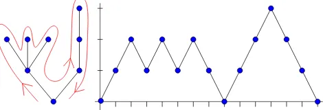
which may be informally described as follows. Consider a plane tree τ ∈Tn (see Figure 2), and
a fly walking around the treeτ clockwise, starting from the root, at the speed 1 edge per unit of time. LetV(t) be the distance from the root to the fly at timet. The process V(t) is called in the literature, the contour process or the Harris’ walk associated with τ. The contour process
Figure 2: A plane tree and its contour process
is the very important tool for the study of plane trees and their asymptotics and we refer to Aldous (1), Pitman (21, Section 6), Duquesne & Le Gall (10), Marckert & Mokkadem (16) for considerations on the asymptotics of normalized trees. It is straightforward that the set of trees encoded byE2n(k)is the subset ofTnof trees having exactlykleaves (sayTn(k)), a leaf being a node
without any child. A corollary of Theorem 4, is that random plane tree with n edges and K2n
leaves, converges, normalized by β2n/2, to the continuum random tree introduced by Aldous
(1), which is encoded by 2e. The variable Λ2nt gives the number of leaves visited at time 2nt.
By Theorem 4, supt∈[0,1]|(Λ2nt−tK2n)/n|proba.−→ 0. This translates the fact that the leaves are
asymptotically uniformly distributed on a random tree chosen equally likely inT(K2n)
1.2 Consequences in terms of parallelogram polyominoes
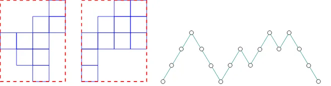
We refer to Delest & Viennot (8) for more information on parallelogram polyominoes. Unit squares having their vertices at integer points in the Cartesian plane are called cells. A polyomino is a finite union of cells with connected interior. The number of cells is the area and the length of the border is called the perimeter (see Figure 3). A polyomino P is said to be convex if the intersection of P with any horizontal or vertical line is a convex segment. For any convex polyomino P there exists a minimal rectangle R(P) (that can be seen as a convex polyomino) containing P. Then P touches the border of R(P) along four connected segments. A convex polyominoP is said to be a parallelogram polyomino if the south-west point and the north-east point of R(P) belong to P (see Figure 3). Let denote by H(P) and V(P) the horizontal and
Figure 3: The first convex polyomino is not parallelogram, the second is. Their areas are 9 and 11, their perimeters equal that of their minimal rectangles, here 18. For both polyominoes
H(P) = 4 andV(P) = 5. The last picture represents the Bernoulli excursion associated byρ
with the parallelogram polyomino.
vertical length of the border ofR(P), and let Polnbe the set of parallelogram polyominoes with
perimeter n.
Proposition 6. (Delest & Viennot (8, Section 4)) For any integer N ≥1, there is a bijectionρ betweenE2N and Pol2N+2, such that ifP =ρ(S), the area of P is equal to the sum of the heights
of peaks of S, moreover #S∧ =H(P), and V(P) = 2N + 2−2#S∧ (where 2N −2#S∧ is the number of steps of S that do not belong to a peak).
By symmetry with respect to the first diagonal, the random variablesV(P) and H(P) have the same distribution whenP is taken equally likely in Pol2N+2. Hence, the proposition says that
underPe2N, 2N+ 2−2#S∧ and #S∧ have the same distribution.
We describe in a few words Delest & Viennot’s bijection: the successive lengths of the columns of the polyomino P give the successive heights of the peaks of S. The difference between the heights of the floor-cells of theith andi+ 1th columns ofP plus one gives the number of down steps between theith andi+ 1th peaks ofS.
For i ∈ {1, . . . , H(P)}, let vi(P) be the number of cells in the ith column of P. The values
(vi(P))i∈J1,H(P)K coincide with the ordered sequence (Si)i∈S∧. LetP (Kn)
on the set of parallelogram polyominos with perimeter 2n+ 2 and width Kn (that is such that
H(P) =Kn). Assume thatv is interpolated between integer points, and v(0) = 0. We have
Proposition 7. If (Kn) satisfies (H), under P(P ol(2n+2)Kn)
v(Knt)
βn
t∈[0,1] (d)
−→(et)t∈[0,1]
in C[0,1]endowed with the topology of uniform convergence.
Proof. Let (Vi)i∈{1,...,Kn} be the successive height of the peaks in S. Assume also that
V(0) = 0 and that V is interpolated between integer points. By Delest & Viennot’s bijec-tion, βn−1v(Kn.) under PP ol(2n+2)(Kn) has the same distribution asβn−1V(Kn.) under P
e,(Kn)
n . Since
(βn−1S(nt))t∈[0,1]−→(d) (et)t∈[0,1], to conclude, it suffices to show that
sup
t∈[0,1]
V(Knt)−S(nt)
βn
proba.
−→ 0. (10)
LetJ(i) be (abscissa of) theith peak inS. We have, for anyt∈ {0,1/Kn, . . . ,Kn/Kn},
V(Knt)−S(nt) =S(J(Knt))−S(nt). (11)
As one can see using the convergence ofλn tobb,
sup
t
J(Knt)−nt
n
proba.
−→ 0. (12)
Indeed, supt|J(Knt)−nt|/n≤supt|Λnt−tKn|/nproba.−→ 0. Since (sn) converges inC[0,1] under Pe,(Kn)
n , by a simple argument about its modulus of continuity, using (11) and (12), formula (10)
holds true. ✷
We would like to point out the work of de Sainte Catherine & Viennot (9), who exhibit a quite unexpected link between the cardinalities of excursions having their peaks in a given subset of
Nand the famous Tchebichev polynomials.
1.3 Consequences in terms of Kolmogorov-Smirnov statistics
We refer again to Krattenthaler (14, Example 3.3.2 and Theorem 3.4.4).
Let X = (X1, . . . , Xn) and Y = (Y1, . . . , Yn) be two independent sets of independent random
variables, where theXi (resp. theYi) are identically distributed. Assume that the cumulative
distributions FX and FY of the Xi’s and Yi’s are continuous, and that we want to test the
Let Z = (Z1, . . . , Z2n) be the order statistics of (X1, . . . , Xn, Y1, . . . , Yn); in other wordsZi is
the ith smallest element in (X1, . . . , Xn, Y1, . . . , Yn). We may associate almost surely to Z a
Bernoulli bridgeS ∈ B2n saying thatS(i)−S(i−1) = 1 orS(i)−S(i−1) =−1 whetherZi is
inX or inY.
It is easy to see thatS is uniform in B2n (for anyn) whenFX =FY and that it is not the case
when FX 6=FY: assume thatFX(x)6=FY(x) for somex and denote by NX(x) = #{i, Xi ≤x}
and NY(x) = #{i, Yi ≤x}. By the law of large numbers
NX(x)
n
(a.s.)
−−−→
n FX(x) and
NY(x)
n
(a.s.)
−−−→
n FY(x)
which implies thatS(NX(x)+NY(x)) is at the first ordern(FX(x)−FY(x)), that is much bigger
than the√norder expected by Theorem 2. We examine now, as in (14) the run statistics
Rn(S) = #{i∈J1,2n−1K, S(i+ 1)6=S(i)}
that counts the number of runs in S(up to at most 1, twice the number of peaks) and
Dn,n+ (S) = 1
nmaxi S(i) and Dn,n(S) =
1
nmaxi |S(i)|,
the one-sided and two-sided Kolmogorov-Smirnov statistics.
The run statistics Rn has been introduced by Wald and Wolfowitz (24). It is shown to be
independent ofFX whenFX =FY. It is well adapted in many cases since no assumption onFX
(but its continuity) is needed. Theorem 3.4.4 of Krattenthaler (14) (see also the consideration just above Example 13.3.3) provides the exact enumeration of Bernoulli walks S for which Dn,n ≤t/nand Rn=j.
The random variableRn satisfies obviously
|Rn−2Λ2n| ≤1. (13)
A simple consequence of assertion (7) and (13) is the following result
Corollary 8. If FX =FY then √
n
√
2 D
+ n,n,
√
n
√
2 Dn,n,
Rn−n/2
√
n
(d)
−−→
n (supb,sup|b|, N)
where b is a Brownian bridge independent of N, a centered Gaussian random variable with variance 1/2.
This means that asymptotically the run statistics and the Kolmogorov statistics are independent.
Comments1. Notice that the process t7→Λnt can also be used to build a test H based on the
2
Combinatorial facts : decomposition of trajectories
The decomposition of the trajectories is determinant in our approach, since we will prove directly the convergence of finite dimensional distributions underPnx. An important difference with the case where the peaks are not considered is that under Pnx,(k),S is not a Markov chain. Indeed, the law of (S(j))l≤j≤n depends on S(l), on the number of peaks in J0, lK, and also on the step
(S(l−1), S(l)). The computation of the distributions of vector (S(t1), . . . , S(tk)) in these various
cases admits the complication that S may own a peak in some of the positions t1, . . . , tk. In
order to handle the contribution of these peaks, we have to specify what the types u ord (+1 or−1) of the first and last steps of the studied parts (S(ti), . . . , S(ti+1)) are.
We set the following notation : ∆Sl=S(l)−S(l−1), and write for convenience, ∆Sl=uwhen
∆Sl= 1, and ∆Sl=dwhen ∆Sl =−1. In this paper, we deal only with discrete trajectories S
such that ∆Sk∈ {+1,−1}for anyk. We will not recall this condition.
Foraand bin {d, u}, andl, x, y, j inZ, set
Tabj(l, x, y) = {S :S= (S(i))0≤i≤l, #S∧ =j, ∆S1=a, ∆Sl =b, S(0) =x, S(l) =y}
Tabj,≥(l, x, y) = {S :S∈Tabj (l, x, y), S(i)≥0 for any i∈J0, lK}.
For anyl, j1, j2, x, y ∈Z, set
l, j1, j2, x, y=
l+y−x
2 −1
j1
l−y+x
2 −1
j2
.
We have
Proposition 9. For any y ∈Z, l≥0, j≥0,
#Tabj (l,0, y) =l, j−1b=d, j−1a=u,0, y
. (14)
For any x≥0, y≥1, l≥0,j ≥0,
#Tuuj,≥(l, x, y) = l, j, j−1, x, y−l, j−1, j, −x, y,
#Tudj,≥(l, x, y) = l, j−1, j−1, x, y−l, j−2, j, −x, y,
For any x≥1, y≥1, l≥0,j ≥0,
#Tduj,≥(l, x, y) = l, j, j, x, y−l, j, j, −x, y,
#Tddj,≥(l, x, y) = l, j−1, j, x, y−l, j−1, j, −x, y
(notice that #Tdbj,≥(l,0, y) = 0 and #Tauj,≥(l, x,0) = 0). In other words
Proof. Let n, k∈ N. A composition of n in k parts is an ordered sequence x1, . . . , xk of non
negative integers, such thatx1+· · ·+xk =n. The number of compositions of nin kparts (or
of compositions ofn+kink positive integer parts) is n+kk−−11.
We call run of the chain S = (S(i))0≤i≤l, a maximal non-empty interval I of J1, lK such that
(∆Si)i∈I is constant. The trajectories S of Tabj (l, y) are composed by j+1b=u runs of u and
j+1a=druns ofd. Theu-runs form a composition of (l+y)/2 (this is the number of stepsu) in
positive integer parts, and thed-runs form a composition of (l−y)/2 in positive integer parts. Hence,
#Tabj (l, y) =
(l+y)/2−1 j+1b=u−1
(l−y)/2−1 j+1a=d−1
,
and Formula (14) holds true.
The proofs of the other formulas are more tricky; the main reason for it is that the reflexion principle does not conserve the number of peaks. What still holds is, for any x ≥ 0, y ≥ 0, j≥0, l≥0
#Tabj,≥(l, x, y) = #Tabj(l, x, y)−#Tabj,(l, x, y)
whereTabj,(l, x, y) is the set of trajectories belonging toTabj(l, x, y) that reach the level−1. Since #Tabj (l, x, y) = #Tabj(l,0, y−x) is known, it remains to determineTabj,(l, x, y).
We define two actions on the set of chains :
letS= (S(i))i∈J0,lK∈ Wl. For anyt∈J0, lKwe denote byS′ = Ref(S, t) the pathS′ = (Si′)0≤i≤l obtained fromS by a reflexion from the abscissat; formally :
(
S′(i) =S(i) for any 0≤i≤t,
S′(i+t) = 2S(i)−S(i+t) for any 0≤i≤l−t .
Whengis a function fromWltaking its values inJ0, lK, we write simply Ref(., g) for the reflexion
at abscissag(S).
letS= (S(i))i∈J0,lK∈ Wl. For anycanddinN, 0≤c≤d≤l, we denote byS′ = Cont(S,[c, d])
the pathS′= (S′(i))0≤i≤l−d obtained from S by a contraction of the interval [c, d] : (
S′(i) =S(i) for any 0≤i≤c,
S′(c+i) =S(d+i)−S(d) +S(c) for any 0≤i≤l−(d−c) .
As before, we write Cont(.,[g1, g2]) for the contraction of the interval [g1(S), g2(S)].
We denote by T−1(S) = inf{j : S(j) = −1} the hitting time of −1 by S. We proceed to a
classification of the paths S from Tabj,(l, x, y) according to the two first steps following T−1(S),
that exist since y is taken positive. We encode these two first steps following T−1 above the
symbolT : for anyα, β∈ {u, d}, set
(αβ)
T
j,
t
that this last operation does not create any peak because ∆ST−1(S) = d. The cardinalities of
the sets in the right hand side are known, hence, (du)T dd, (du)
T ud, (du)
T du, (du)
2.1 Proof of Proposition 1
(i) To build a path with k peaks, dispose k peaks, that is k pairs ud. Take a composition x1, . . . , x2(k+1) of n−2kin 2(k+ 1) non negative parts. Fill in now thek+ 1 intervals between
these peaks : in thelth interval disposex2l−1 stepsdand x2l stepsu.
(ii) Assume n = 2N is even. To build a bridge with k peaks, dispose k pairs ud. Take two compositionsx1, . . . , x(k+1)andx′1, . . . , x′(k+1)ofN−kink+ 1 parts. Fill now thek+ 1 intervals
between these peaks : in thelth interval disposexl stepsdand x′l stepsu.
(iii) #En(k)= #Tudk,≥(n−1,0,1) + #Tuuk−1,≥(n−1,0,1)
For (iv), one may use the bijections described in Section 4.4, or proceed to a direct computation as follows; first,
#M(k)n = #En(k)+ X
y≥1
Tuuk,≥(n,0, y) +Tudk,≥(n,0, y). (16)
Denote byW(n, k) the sum in (16). The integerW(n, k) is the number of meanders with length n, ending in a positive position. Using that nk+ k−n1= n+1k , we have
Leta, b, c, k be positive integers, the following formula holds
X
Indeed: a term in the first sum counts the number of ways to choose 2kitems amonga+b+ 1, choosing, the a+y+ 1th, and k items among the a+y first ones, when, a term in the second sum counts the number of ways to choose 2kitems amonga+b+ 1, choosing, thea+y+ 1th, andk−1 items among thea+yfirst ones. The choices counted by the first sum but not by the second one, are those where exactly kitems are chosen among thea+c first ones.
We need to consider the two casesneven andn odd :
3
Asymptotic considerations and proofs
We first recall a classical result of probability theory, simple consequence of Billingsley (6, Theorem 7.8), that allows to prove the weak convergence inRdusing a local limit theorem.
Proposition 10. Let k be a positive integer and for each i ∈ J1, kK, (α(i)n ) a sequence of real
numbers such that α(i)n −→
n +∞. For any n, let Xn = (X (1)
n , . . . , Xn(k)) be a Zk-valued random
variable. If ∀λ= (λ1, . . . , λk)∈Rk,
α(1)n . . . α(k)n P (Xn(1), . . . , Xn(k)) = (⌊λ1α(1)n ⌋, . . . ,⌊λkα(k)n ⌋)
−→φ(λ1, . . . , λk)
where φ is a density probability on Rk, then (Xn(1)/α(1)n , . . . , Xn(k)/α(k)n ) (d)
−−→
n X where X is a
random variable with density φ.
Proposition 3 is a simple consequence of this proposition, since by (1) and Proposition 1, the application of the Stirling formula simply yields
√
nPnx(⌊Λn−n/4⌋=⌊t√n⌋)−−→ n
1
p
2π/16exp(−8t
2),
for anyx∈ {w,b,e,m} and anyt∈R. Note that underPw
n, one may also compute the limiting
distribution using that Λn(S) =Pni=1−11i∈S∧, which is a sum of Bernoulli random variables with
an easy to handle dependence.
3.1 Finite dimensional distribution of the Brownian processes
Notation For any sequence (oi)i indexed by integers, the sequence (∆oi) is defined by ∆oi =
oi−oi−1 and (∆oi) by ∆oi =oi+oi−1.
For anyt >0 andx, y∈R, set
pt(x, y) =
1
√
2πtexp
−(y−x)
2
2t
.
Letℓ≥1 and let (t1, . . . , tℓ)∈[0,1]ℓsatisfying 0< t1<· · ·< tℓ−1< tℓ := 1. The distributions of
the a.s. continuous processesw,b,e,mare characterized by their finite dimensional distributions. Letfx
t1,...,tk be the density of (xt1, . . . ,xtk) with respect to the Lebesgue measure on R
k. We have
fw
t1,...,tℓ(x1, . . . , xℓ) =
ℓ Y
i=1
p∆ti(xi−1, xi), withx0 = 0 by convention,
ft1b,...,tℓ−1(x1, . . . , xℓ−1) =
√
2π ft1,...,tw ℓ−1(x1, . . . , xℓ−1)p∆tℓ(xℓ−1,0),
ft1,...,tm ℓ(x1, . . . , xℓ) =
√
2πx1 t1
pt1(0, x1) ℓ Y
i=2
p∆ti(xi−1, xi)−p∆ti(xi−1,−xi)
!
1x1,...,xℓ≥0,
fe
t1,...,tℓ−1(x1, . . . , xℓ−1) = f
m
t1,...,tℓ−1(x1, . . . , xℓ−1)
xℓ−1
∆tℓ
We end this section with two classical facts: first pt(x, y) = pt(0, y −x) and, for any α > 0,
fαx
t1,...,tk(x1, . . . , xk) =α
−kfx
t1,...,tk(x1/α, . . . , xk/α).
3.2 Finite dimensional convergence
We will show that for anyx∈ {w,b,e,m}, underPnx, for anyℓ∈ {1,2,3, . . .}and 0< t1 <· · ·<
tℓ−1< tℓ:= 1
(sn(t1), . . . , sn(tℓ), λn(t1), . . . , λn(tℓ)) (d)
−−→
n
x(t1), . . . ,x(tℓ),bb(t1), . . . ,bb(tℓ)
,
wheretℓ:= 1 has been chosen for computation convenience, and (x,bb) has the prescribed
distri-bution (as in Theorem 4). This implies the convergence of the finite dimensional distridistri-bution in Theorem 4.
In order to handle easily the binomial coefficients appearing inl, j1, j2, x, ythat involve half
in-tegers, we proceed as follows. LetN =⌊n/2⌋and letEn=n−2N =n mod 2. Fori∈J1, ℓ−1K,
lett(n)i be defined by
2N t(n)i := 2⌊nti/2⌋,
t(n)0 = 0, andt(n)ℓ by 2N t(n)ℓ = 2N+En=n(notice that t(n)ℓ is in {1,1 + 1/(n−1)}).
Using that for anyi,|2N t(n)i −nti| ≤2, we have clearly underP
x,(Kn)
n ,
S(2N t(n)i )−S(nti)
βn
proba.
−→ 0 and Λ
2N t(in) −
Λnti
γn
proba.
−→ 0 (18)
since γn and βn goes to +∞. From now on, we focus on the values of the processes on the
discretization points 2N t(n)i . For anyi∈J1, ℓ−1K, set
e
Λi := #S∧∩J2N t(n)i−1+ 1,2N t (n) i −1K
the number of peaks lying strictly between 2N t(n)i−1 and 2N t(n)i .
In order to obtain a local limit theorem, we are interested in the number of trajectories passing via some prescribed positions.
3.2.1 Case x=w
Let 0 =u0, u1, . . . , uℓ, v1, . . . , vℓ−1 be fixed real numbers. Set
Θ := (t1, . . . , tℓ−1, u1, . . . , uℓ, v1, . . . , vℓ−1)
and for anyi∈J1, l−1K, set
and
increments of the ith part of S between the discretization points. Some peaks may appear in the positions 2N tni, and then, we must take into account the pairs (bi, ai+1) to compute the
In order to evaluate the sum (19), we introduce some binomial random variablesB(l, pn) with
parametersl and pn and we use the following version of the local limit theorem
Lemma 11. Let (l(n)) be a sequence of integers going to +∞ and σn2 = l(n)pn(1−pn). We
We then get easily that
#TK(ni)
is equivalent to π∆t1
is equivalent to π∆t1
The contribution of the sum overc has been computed as follows:
X
−→ 0, this allows to conclude to the finite dimensional convergence in The-orem 4 in the casex=w.
Comments 2. To compute a local limit theorem under the other distributions the numbers u1, . . . , uℓ, v1, . . . , vℓ and the set Awn have to be suitably changed. First, in each case, the set
W(Kn)
n has to be replaced by the right set.
• In the case of excursions and bridges, nis an even number and uℓ is taken equal to 0.
• In the case of excursions a1 =u, bℓ=d
• In the case of excursions and meanders all the reals ui are chosen positive. Moreover, T≥
must replace T in the summation (19).
Up to these changes, the computations are very similar to the case of Bernoulli chains.
3.2.2 Case x=b
wherecb
formulas provided in Proposition 9 that have to be handled with precautions whenxory are 0, we will compute the local limit theorem “far” from 0. This will however suffice to conclude. For i∈J1, ℓ−1Kwe takeui >0, andβnis assumed large enough so that⌊uiβn⌋>0. For the calculus
in the case ofx=e, in formula (19), we replace T byT≥. Finally, #E(Kn)
n = N1 KNn KnN−1.
We first treat the contribution of the non extreme parts of the trajectories, namely,i∈J2, l−1K,
#TK(
We notice that under (H)
n=o(Knβn), γn=o(n−2Kn), γn≤βn, γn=o(Kn).
The casei=ℓis treated with the same method. We obtain
Pe,(Kn)
type as a standard excursion piece. We obtain
4
Tightness
We begin with some recalls of some classical facts regarding tightness in C[0,1]. First, tight-ness and relative compacttight-ness are equivalent in C[0,1] (and in any Polish space, by Prohorov). Consider the function modulus of continuity,
ω: [0,1]×C[0,1] −→ R+
(δ, f) 7−→ ωδ(f)
defined by
ωδ(f) := sup s,t∈[0,1],|s−t|≤δ|
f(t)−f(s)|.
A sequence of processes (xn) such thatxn(0) = 0 is tight inC[0,1], if for anyε >0, η >0, there
existsδ >0, such that fornlarge enough
P(ωδ(xn)≥ε)≤η.
If the sequences (xn) and (yn) are tight inC[0,1] (and if for each n, xn and yn are defined on
the same probability space Ωn), then the sequence (xn, yn) is tight inC([0,1])2. We will use this
result here, and prove the tightness separately for (sn) and (λn) for every model Pxn.
We say that a sequence (xn) inC[0,1] is tight on [0,1/2] if the sequence of restrictions (xn|[0,1/2])
is tight inC[0,1/2]. We would like to stress on the fact that we deal only with processes piecewise interpolated (on intervals [k/n,(k+ 1)/n]); for these processes, for n large enough such that 1/n < δ,
sup{|xn(t)−xn(s)|, s, t∈ {k/n, k∈J0, nK},|s−t| ≤δ} ≤ε/3
⇒(ωδ(xn)≤ε).
In other words, one may assume thatsandtare discretization points, in our proofs of tightness.
We recall a result by Petrov (19, Exercise 2.6.11) :
Lemma 12. Let (Xi)i be i.i.d. centered random variables, such that E(etX1) ≤egt 2/2
for |t| ∈
[0, T]and g >0. Let Zk=X1+· · ·+Xk. Then
P( max
1≤k≤N|Zk| ≥x)≤2 (
exp(−x2/2N g) for anyx∈[0, N gT] exp(−T x) for any x≥N gT.
The tightness of (sn, λn) is proved as follows: first, underP
w,(Kn)
n , the passage via an alternative
model of “simple random walk” allows to remove the conditioning by Λn=Kn. Then, the
tight-ness underPb,(Kn)
n is deduced from that underP
w,(Kn)
n , thanks to the fact that the conditioning by
S(n) = 0 does not really change the distribution the first half of the trajectories. The tightness under Pe,(Kn)
n and P
m,(Kn)
n are then obtained from that under P
b,(Kn)
n by some usual trajectory
4.1 A correspondence between simple chains and Bernoulli chains
We denote byHn the set of “simple chains”, starting from 0 and havingn+ 1 steps :
Hn={H= (Hi)0≤i≤n+1 :H0= 0, Hi+1=Hi orHi+1=Hi+ 1 for anyi∈J0, nK}.
We consider the map
Φn: Wn −→ Hn
S 7−→ H= Φn(S)
whereHis the simple chain with increments: for any i∈J1, n+ 1K,
(
if ∆Si 6= ∆Si−1 then ∆Hi= 1
if ∆Si = ∆Si−1 then ∆Hi= 0
where by convention ∆S0 =−1 and ∆Sn+1= 1 (see illustration on Figure 5).
0
S
H
2 4 6
n+ 1
Figure 5: Correspondence between simple chains and Bernoulli chains
The mapping Φn is a combinatorial trick. Obviously, the map S 7→ H where H is defined by
∆Hi = (∆Si + 1)/2 is a bijection from Wn onto Hn−1. The map Φn is then certainly not a
bijection (it is an injection). But, Φn owns some interesting properties that will really simplify
our task.
Each increasing step in H corresponds to a changing of direction in S. Since ∆S0 = −1, the
first one corresponds then to a valley, and the last one to a valley (which can not be in position n, since ∆Sn+1 = 1). Hence, for anyj∈J0, nK,
Λj(S) = #S∧∩J0, jK=
Hj+1
2
.
Hence,
where (−S)∧ is the set of valleys of S and where Tl(H) = inf{j, Hj =l} is the hitting time by
Hof the levell. The process S may then be described withH:
S(k) =
HXk−1
i=0
(−1)i+1(Ti+1(H)− Ti(H)) + (−1)Hk+1(k− THk(H)). (21)
To end these considerations, consider now the subset of simple chains withk increasing steps,
Hk
n={H∈ Hn, Hn+1=k},
and focus onH2k+1
n . Each elementH∈ H2k+1n is image by Φn of a unique trajectorySthat has
kpeaks inJ1, n−1Kandk+ 1 valleys inJ0, nK(that may be in position 0 andnby construction), in other words, to a trajectory of Wn(k).
This may alternatively be viewed as follows: to build a trajectory ofWn(k)choose 2k+ 1 integers
i1 < i2 <· · ·< i2k+1 in the set J0, nK. Then construct a trajectory from Wn in placing a valley
ini1, i3, . . . , i2k+1, a peak in i2, i4, . . . , i2k and fill in the gaps between these points by straight
lines. Hence
Lemma 13. For any k∈J0,⌊n/2⌋K, the restriction of Φn on Wn(k) is a bijection onto H2k+1n .
For any p ∈[0,1], let Qnp be the distribution on Hn of the Bernoulli random walks withn+ 1
i.i.d. increments, Bernoulli B(p) distributed (that is Qnp(∆Hi = 1) = 1−Qnp(∆Hi = 0) = p).
For anyHinHn,
Qnp({H}) =pHn+1(1−p)n+1−Hn+1,
and then, Qnp gives the same weight to the trajectories ending at the same level. Hence the conditional distribution Qnp( . |H2k+1
n ) is the uniform law on Hn2k+1. On the other hand, since Pwn,(k) is the uniform distribution on Wn(k), by Lemma 13, P
w,(k)
n ◦Φ−n1 is also the uniform law
on H2k+1
n . Hence
Lemma 14. For any p∈(0,1), n∈N, k∈J0,⌊n/2⌋K, Qnp( . |H2k+1 n ) =P
w,(k)
n ◦Φ−n1.
Using simple properties of binomial distribution, the value of p that maximizes Qnp(H2Kn+1
n )
is ˜pn = (2Kn + 1)/(n+ 1). This morally explains why in Section 3, pn appears as a suitable
parameter. For sake of simplicity, we will work again withpn = 2Kn/n instead of ˜pn. We will
see that under Qnpn, the conditioning by H2k+1n is a “weak conditioning”, and to bound certain quantities, this conditioning may be suppressed, leading to easy computations. The archetype of this remark is the following property
Lemma 15. Assume (H). There exists c > 0 such that for n large enough, for any set An on Hn depending only on the first half part of the trajectories, (that is
σ(H0, H1, . . . , H⌊n/2⌋)−measurable),
e
Qn(An) :=Qnpn(An| H
2Kn+1
Proof. The idea is taken from the proof of Lemma 1 in (12) :
e
Qn(An) = X
j e
Qn(An, H⌊n/2⌋=j)
= X
j Qnp
n(An|H⌊n/2⌋=j, Hn+1 = 2Kn+ 1)Qen(H⌊n/2⌋=j)
= X
j
Qnpn(An|H⌊n/2⌋=j) Qen(H⌊n/2⌋=j).
The latter equality comes from the Markov property of H under Qnpn that implies that
Qnp
n(Hn+1 = 2Kn + 1|An, H⌊n/2⌋ = j) = Q
n
pn(Hn+1 = 2Kn + 1|H⌊n/2⌋ = j). It suffices to
establish that there exists c≥0 such that forn large enough, for anyj
e
Qn(H⌊n/2⌋=j)≤c Qnpn(H⌊n/2⌋=j).
Write
e
Qn(H⌊n/2⌋=j) =Qnpn(H⌊n/2⌋=j)
Qnp
n(H⌊n/2⌋= 2Kn+ 1−j)
Qn
pn(Hn+1= 2Kn+ 1)
;
using Lemma 11, the last quotient is bounded, uniformly onj and n≥1. ✷
A simple consequence of Lemma 15 is the following : letXn be a positive random variable that
depends only on the first half part of the trajectories, then the expectation of Xn under Qen is
bounded by the expectation ofc Xn under Qnpn.
4.2 Tightness under Pw,(Kn)
n
Assume that (Kn) satisfies (H), that S∈ Wn, and let H= Φn(S). Set
hn(t) =
H(n+1)t 2γn −
tKn
γn
fort∈[0,1], (23)
where H is assumed to be interpolated between integer points. Thanks to formulas (4), (5), (21),
|λn(t)−λn(s)| ≤ |hn(t)−hn(s)|+ 2/γn. (24)
Hence, the tightness of (hn) underQen implies the tightness of (λn) underP
w,(Kn)
n .
By symmetry of the random walk under these distributions, we may prove the tightness only on [0,1/2]. By Lemma 15, the tightness of (hn) on [0,1/2] underQnpn implies the tightness of (hn)
on [0,1/2] underQen, and then that of (λn) on [0,1/2] underP
w,(Kn)
n . Hence, it suffices to prove
the tightness of (hn) on [0,1/2] underQnpn to prove that of (λn) on [0,1] underP
w,(Kn)
n .
Comments3. The conditioning by the number of peaks is a strong conditioning on Wn. Indeed,
W(Kn)
n may have a very small (even exponentially small) probability under Pwn when Kn is far
away fromn/4: no tight bound can be derived using comparison between Pwn andPw,(Kn)
n by just
Tightness of the sequence (λn) under P
w,(Kn)
n
At first sight, under Qnpn, (hn) is a random walk with the right normalization, and it should
converge to the Brownian motion (and then the tightness should follow). However, we were unable to find a reference for this result under the present setting. We will then prove it.
In the sub-case where there exists δ >0 such that, for nlarge enough,pn satisfies nδ−1 ≤pn≤
1−nδ−1 then under Qn pn, hn
(d)
−−→
n w in C[0,1] : it is a consequence of Rackauskas, & Suquet
(22, Theorem 2). In this case the tightness holds in a space of H¨older functions, with exponent smaller than 1/2· When pn =o(nδ−1) or 1−pn = o(nδ−1), for anyδ, (hn) is not tight in any
H¨older space; this may be checked by considering a single normalized step.
Letε >0 andη >0 be fixed, and let us prove that for anynlarge enough,Qnp
n(ωδ(hn)≥ε)≤η
forδ sufficiently small. So take a parameter δ ∈(0,1). We have
ωδ(hn)≤2 max
0≤j≤⌊1/(2δ)⌋ maxIδ j(n)
hn−min Iδ
j(n)
hn !
(25)
where
Ijδ(n) =
2j⌊δ(n+ 1)⌋ n+ 1 ∧1,
2(j+ 1)⌊δ(n+ 1)⌋ n+ 1 ∧1
(notice that the length of Ijδ(n) is larger than δ forn large enough, and smaller than 3δ). The factor 2 in (25) simply comes from the splitting up [0,1] into parts. Since the extremities of the Ijδ(n)’s coincide with the discretization points, by the Markov property of hn,
Qnpn(ωδ(hn)≥ε)≤(1/(2δ) + 1)Qnpn
sup
Iδ
0(n)
|hn| ≥ε/2
. (26)
We need to control the supremum of a random walk, and we then use Lemma 12.
Lemma 16. Let B(pn) be a Bernoulli random variable with parameter pn. There existsK >0,
such that for any n≥1, any |t| ≤γn,
E(et(B(pn)−pn)/γn)≤exp
2K n
t2
2
. (27)
Proof. There existsK >0 such that, for any|x| ≤1,ex≤1 +x+Kx2. Hence, for any|t| ≤1, E(et(B(pn)−pn)) =p
net(1−pn)+ (1−pn)e−tpn ≤1 +Kt2(pn(1−pn))≤e2Kt 2p
n(1−pn). Hence, for
any|t| ≤γn, (27) holds (recall that (1−pn)pn/γn2 = 1/n). ✷
Let us end the proof of tightness of (hn). Since, forN ∈J0, nK,hn(N/(n+1)) = 2(n+1)γN pn n+DN/2
whereDN is a sum ofN i.i.d. r.v. with law of (B(pn)−pn)/γn. Notice also that 2(n+1)γN pn n =o(1).
By Lemmas 12 and 16, we get
Qnp
n
sup
j≤N|
Dj| ≥ε/2
Letε >0 andδ >0 be fixed. For nlarge enough,
and this is smaller than anyη >0 for δ small enough, andn large enough.✷
Tightness of (sn) under P
same interval. Denote by yn(s, t) the right hand side of (28). We may control the range of sn
under Pw,(Kn)
Since Hn is a binomial random variable with parameters nand pn = 2Kn/n, by the
Bienaym´e-Tchebichev’s inequality, the first term in the right hand side is O(K−1
n ). For the second term,
write Qnpn supj≤4KnGj(H)≥εβn
= 1−(1−P(G1 ≥ εβn))4Kn. Since P(G1 ≥ εβn) = (1−
pn)⌈εβn⌉−1, we find that the second term goes to 0 whenn→+∞.
It remains to control the variables ˜yn(s, t). Using the Markov property of the random walk
Writing Gei instead ofG2i−G2i−1, we have
Once again, by Bienaym´e-Tchebichev,Qnp
n({H3nδ >12Knδ}) =O(1/(δKn)). For the second set
in the union, we have to control the maximum of a random walk with increments the variables
e
G.
Lemma 17. Let G1 and G2 be two independent geometrical random variables with parameter
pn. There exists c >0, c′ >0, such that for any |t| ≤c′γn,
We end now the proof of tightness for the family (sn). According to Lemmas 12 and 17, for
ε >0, δ >0 fixed, for a constantc′′>0 and nlarge enough
In this section,nis an even number. SincePbn,(k)is the uniform distribution onBn(k), it coincides
with the conditional lawPwn,(k)( .|S(n) = 0). We first establish a lemma that allows to control
the probability of a set underPb,(Kn)
n , by the probability of the same set underP
w,(k)
n .
Lemma 19. Assume (H). Let (αn) be a sequence such that αn → +∞. There exist c > 0,
the first half of the trajectories. By Lemma 15, for any setIn,
Pw,(Kn)
n Λn/2−1(S)∈In=Qen ⌊Hn/2/2⌋ ∈In≤c′′ Qpnn ⌊Hn/2/2⌋ ∈In
.
Under Qnpn, Hn/2 is a binomial random variable with parameters n/2 and pn. Now, using
Lemmas 12 and 16 with In = ∁[Kn/2−αnγn,Kn/2 +αnγn], we get the first assertion. The
second assertion is a consequence of Lemma 18. ✷
ConsiderWn the set of simple walks satisfying
Wn={S:S∈ Wn,
n (Wn) → 1, we will from now on concentrate on these trajectories.
We stress on the fact thatγn5/4 =o(Kn). Assume that the following lemma is proved.
Lemma 20. Assume (H). There exists a constant c >0 such that for n large enough, for any subsetAn ⊂ Wn depending only on the first half of the trajectories,
Pb,(Kn)
This lemma, very similar to Lemma 15, allows to obtain the tightness of (sn, λn) underP
b,(Kn)
n
from that underPw,(Kn)
n ; proceed as follows. By symmetry of bridges underP
b,(Kn)
n on [0,1/2]. It only remains to prove Lemma 20.
Proof of Lemma 20 First, for anyAn, depending only on the first half of the trajectories,
Pw,(Kn)
then the first conditioning byAn may be deleted, by Markov. A trite computation leads to the
We choose to condition by the last increment ofS inJ0, n/2Kfor computation reasons.
For anya∈ {u, d}, denoteT−a=Tua∪Tda and similar notation for Ta− andT− −.
and the right hand side
#Tl
To prove (34) whena=dit suffices to prove that
lim sup
We will prove this assertion by showing that for any sequence (ln) of integers, that satisfies
ln ∈Jn for any n, (Gn(ln)) converges to a constant that does not depend on (ln). This allows
to conclude, since one may take the sequence (ln) s.t. Gn(ln) maximizesGn(l) onJn for any n.
Setρn= 4(Kn−ln)/n. Sinceln∈Jn, for anyn,ρn∈(0,1).Now, one checks easily that
Gn(ln) =
γnP(B(⌊n/4⌋, ρn) =Kn−ln)P(B(⌈n/4⌉, ρn) =Kn−ln) P(B(n/2, ρn) = 2(Kn−ln))
.
Since Kn−ln∼ Kn/2, by the central local limit theorem, it converge to 2/√π.
• Casea=u. In this case, the left hand side of (34) equals
#T−lu(n/2, x,0)(#TKn−l
u− (n/2, x,0) + #TdK−n−l−1(n/2, x,0))
#B(Kn)
n
and the right hand side
#Tl
−d(n/2, x,0)(#W (Kn−l)
n/2,u + #W
(Kn−l−1
n/2,d ))
#W(Kn)
n
,
whereWk
n,a is the set of trajectoriesS withk peaks with ∆S1 =a.
Once again, it suffices to check that the quotient
#TKn−l
u− (n/2, x,0) + #TdK−n−l−1(n/2, x,0) =
1 + n/22−x k−l
n/2+x 2 −1
Kn−l−1
divided by
#WKn−l
n/2,u+ #W
(Kn−l−1)
n/2,d =
n/2 + 1 2(Kn−l)
is bounded byc#B(Kn)
n /#Wn(Kn). The same arguments lead to the same conclusion.✷
4.4 Tightness under Pm,(Kn)
n
The case n even
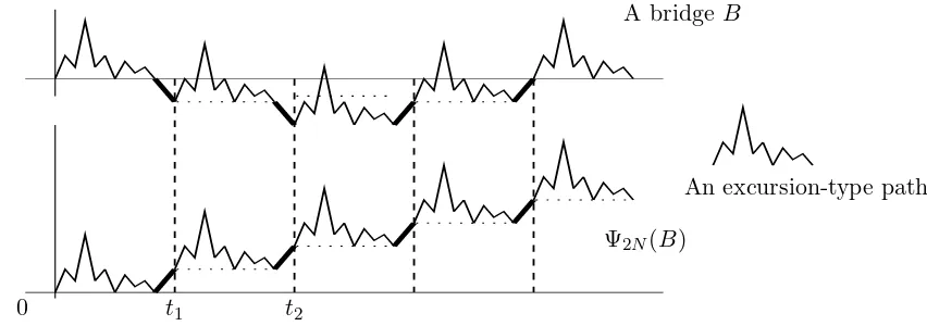
Assume first that n = 2N is even. We recall a bijection Ψ2N : B2N → M2N, illustrated on
Figure 6, that maps B(k)2N on M(k)2N, and that moreover preserves sufficiently the trajectories, to prove that the tightness of (s2N, λ2N) underP
b,(K2N)
2N yields that underP
m,(K2N)
2N .
The map Ψ2N :B2N → W2N (we will see later that Ψ2N(B2N) =M2N) is defined as follows. Let
S ∈ B2N and m = minS ≤0 its minimum. For j ∈ {1, . . . ,−m}, let tj =τ−j(S) the reaching
time of −j byS. WriteIS ={tj, j≥1}. Notice that whenm= 0,IS =∅.
The trajectory Ψ2N(S) =Z= (Zi)i=0,...,nis defined by Z0 = 0 and :
∆Zi = (
∆Si ifi /∈IS,
Proposition 21. For any even2N, Ψ2N is a bijection from B2N ontoM2N; moreover, for any
k, its restriction toB2N(k) is a bijection onto M(k)2N that preserves the peak positions.
Proof. First, it is easy to see that if Z= Ψ2N(S), for anyi≤2N,
Zi =S(i) + 2 min
j≤i S(j). (35)
Hence, Ψ2N(B2N)⊂ M2N. Since Ψ2N is clearly an injection, the first assertion of the Proposition
follows #B2N = #M2N. Since Ψ2N neither creates nor destroys any peaks, nor even changes
the position of the peaks, the restriction of Ψ2N ontoB2N(k) is a bijection onto Ψ2N(B2N(k))⊂ M (k) 2N.
The equality #B2N(k) = #M(k)2N suffices then to conclude. ✷
An excursion-type path A bridge B
Ψ2N(B)
0 t1 t2
Figure 6: Synthetic description ofΨ2N. The mapΨ2N turns over each increment corresponding
to a reaching time of a negative position. The mapΨ−1
2N turns over the last increments reaching
each positionx∈J1, Z2N/2K(Z2N is even).
By Proposition 21, the tightness of (λ2N) underP
m,(K2N)
2N is a consequence of that underP
b,(K2N)
2N .
For (s2N), (35) implies that the modulus of continuity of the non normalized trajectories are
related by
ωZ(δ)≤3ωS(δ) for anyδ∈[0, n]
and then, the tightness of (s2N) under P
m,(K2N)
2N follows that underP
b,(K2N)
2N .
The case n odd
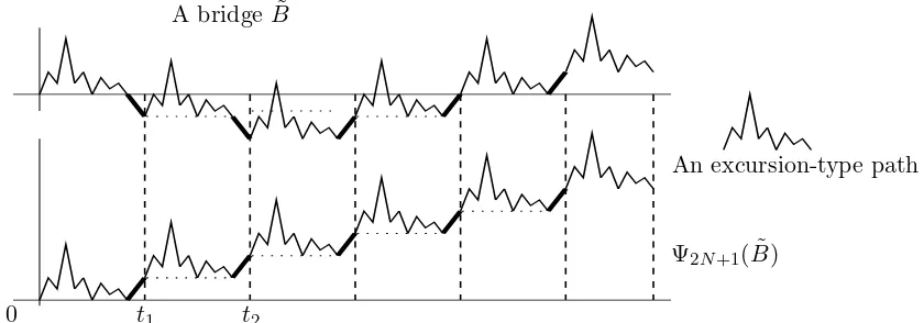
The case n = 2N + 1 odd is very similar. There exists a bijection Ψ2N+1 betweenBe2N+1 and
M2N+1 where Be2N+1 is the subset of W2N+1 of trajectories ending at position +1. The map
Ψ2N+1 has the same properties as Ψ2N to conserve the peak positions, and the set ˜B(2N+1K2N+1):= e
B2N+1∩ W2N+1(K2N+1) is sent onM(2N+1K2N+1). To conclude, we need a tightness result for the uniform
distribution on ˜B(K2N+1)
2N+1 . But the result of Section 4.3 regarding B (K2N)
2N may be generalized to
B(K2N+1)
An excursion-type path A bridge ˜B
Ψ2N+1( ˜B)
0 t1 t2
Figure 7: Synthetic description of Ψ2N+1. The map Ψ2N+1 turns over each increment
cor-responding to a reaching time of a negative position. The map Ψ−1
2N+1 turns over the last
increments reaching each positionx∈J1,⌊Z2N+1/2⌋K(Z2N+1 is odd).
Hence, (s2N+1, λ2N+1) is tight underP
m,(K2N+1)
2N+1 , and then we may conclude that (sn, λn) is tight
underPm,(Kn)
n .
4.5 Tightness under Pe,(Kn)
n
Here n= 2N is an even number. Consider
ˇ
B2N+1 = {S,S∈ W2N+1, S(2N + 1) =−1},
ˇ
E2N+1 = {S,S∈ W2N+1, S(j)≥0 for anyj∈J0,2NK, S(2N + 1) =−1}
and ˇB2N(K)+1 = ˇB2N+1 ∩ W2N+1(K) , ˇE (K)
2N+1 = ˇE2N+1 ∩ W2N+1(K) . Informally, ˇE2N+1 (resp. ˇE2N(K)+1)
are Bernoulli excursion from E2N (resp. with K peaks) with an additional ending d-step, and
ˇ
B2N+1 and ˇB2N+1(K) are trajectories ending at −1 (resp. withK peaks).
Consider the map
R: Eˇ2N+1×J0,2NK −→ Bˇ2N+1
(S, θ) 7−→ R(S, θ) =S(θ)= (S(θ))
i=0,...,2N+1
defined by
∆Sk(θ)= ∆Sk+θ mod 2N+1
or equivalentlySk(θ) =S(k+θ mod 2N+1)−S(θ)−1k+θ>2N+1. Informally,S7→S(θ)exchanges
the θ first steps of S with the last 2N + 1 −θ’s ones. The map R is a bijection between ˇ
E2N+1 ×J0,2NK and ˇB2N+1: this is the so-called cyclical lemma attributed to
iffθ∈S∧ (ifθ /∈S∧ then #S(θ)∧ = #S∧).
For anyS∈ W2N+1, set Ξ0(S) = 0, and for anyk≤2N−#S∧,
Ξm(S) := min{j, j≥Ξm−1(S), j≤2N, j /∈S∧},
the successive non-peak positions of S inJ0,2NK. Consider the map
b
R: Eˇ2N(K)+1×J0,2N−KK −→ Bˇ2N(K)+1
(S, ℓ) 7−→ Rb(S, ℓ) =S(Ξℓ(S)) .
Proposition 22. For anyK ≤N, anyN ≥0, the mapRb is a bijection fromEˇ2N(K)+1×J0,2N−KK
onto Bˇ(K)2N+1.
Proof. It is a consequence of the two following points: for any S, m 7→ Ξm(S) is a bijection
from J0,#J0,2NK\S∧Konto J0,2NK\S∧, and Ris a bijection.✷
Consider (S, θ) in ˇE2N+1(K) ×J0,2N −KK; for anyu,
sup
|m1−m2|≤u|
S(m1)−S(m2)| ≤ 2 sup |m1−m2|≤u|
S(θ)(m1)−S(θ)(m2)| (36)
sup
|m1−m2|≤u
(Λm1 −Λm2)(S)−
m1−m2
2N K2N
≤ 2 sup |m1−m2|≤u
(Λm1−Λm2)(S(θ))−
m1−m2
2N K2N
.
Endow ˇE2N+1(K) ×J0,2N−KKwith the uniform distribution and consider a random element (S, θ) under this law (Sis then uniform on ˇE2N+1(K) ). By the last proposition,S(θ)is uniform on ˇB2N(K)+1. By (36), we have
Pe,(K2N)
2N (ωδ(s2N)≥ε)≤P
w,(K2N)
2N+1 (2ωδ(s2N)≥ε|S(2N + 1) =−1)
and the same result holds for λ2N. Once again the result of Section 4.3 concerning P
b,(K2N)
2N =
Pw,(K2N)
2N (.|S(2N = 0)) can be generalized toP
w,(K2N)
2N (.|S(2N + 1) =−1). ✷
Acknowledgments
We would like to thank Mireille Bousquet-M´elou who pointed many references, and for helpful discussions. We thank the referee for pointing out some important references.
References
[1] D. Aldous, (1991) The continuum random tree. II: An overview., Stochastic analysis, Proc. Symp., Durham/UK 1990, Lond. Math. Soc. Lect. Note Ser. 167, 23-70. MR1166406
[3] J. Bertoin, L. Chaumont & J. Pitman, (2003) Path transformations of first passage bridges, Elec. Comm. in Probab.,8, Paper 17. MR2042754
[4] J. Bertoin, & J. Pitman, (1994) Path transformations connecting Brownian bridge, excursion and meander, Bull. Sci. Math., II. S´er. 118, No.2, 147-166.
[5] Ph. Biane, & M. Yor (1987) Valeurs principales associ´ees aux temps locaux browniens., Bull. Sci. Math. (2) 111 (1987), no. 1, 23–101.
[6] P. Billingsley, (1968)Convergence of probability measures, New York-London-Sydney-Toronto: Wiley and Sons. MR0233396
[7] E. Cs´aki & Y. Hu, (2004)Invariance principles for ranked excursion lengths and heights., Electron. Commun. Probab. 9, 14-21.
[8] M.P. Delest, & G. Viennot, (1984) Algebraic languages and polyominoes enumeration., Theoret. Comput. Sci. 34, No. 1-2, 169–206. MR0774044
[9] M. de Sainte Catherine, G. Viennot, (1985)Combinatorial interpretation of integrals of products of Hermite, Laguerre and Tchebycheff polynomials. in “Polynˆomes orthogonaux et applications,” Proc. Laguerre Symp., Bar-le- Duc/France 1984, Lect. Notes Math. 1171, 120-128.
[10] T. Duquesne, & J.F. Le Gall (2002)Random trees, L´evy processes and spatial branching processes, Ast´erisque, 281. MR1954248
[11] D.L. Iglehart (1974)Functional central limit theorems for random walks conditioned to stay positive.·, Ann. Probability 2, 608–619.
[12] S. Janson & J.F. Marckert, (2005) Convergence of discrete snake., J. Theor. Probab. 18, No.3, 615-645. MR2167644
[13] W.D.Kaigh, (1976),An invariance principle for random walk conditioned by a late return to zero., Ann. Probability 4, No. 1, 115–121. MR0415706
[14] C. Krattenthaler, (1997), The enumeration of lattice paths with respect to their number of turns, Advances in combinatorial methods and applications to probability and statistics, Stat. Ind. Technol., Birkh¨auser Boston, 29–58. MR1456725
[15] T.M. Liggett, (1968),An invariance principle for conditioned sums of independent random variables, J. Math. Mech. 18, 559–570. MR0238373
[16] J.F. Marckert & A. Mokkadem, (2003)The depth first processes of Galton-Watson trees converge to the same Brownian excursion., Ann. of Probab., Vol. 31, No. 3. MR1989446
[17] P. Marchal, (2003)Constructing a sequence of random walks strongly converging to Brownian motion, 181–190 (electronic), Discrete Math. Theor. Comput. Sci. Proc., AC, Assoc. Discrete Math. Theor. Comput. Sci. MR2042386
[18] T.V. Narayana, (1959)A partial order and its applications to probability theory, Sankhy¯a, 21, 91–98. MR0106498
[19] V.V. Petrov, (1995)Limit theorems of probability theory. Sequences of independent random variables., Oxford Studies in Probab. MR1353441
[20] J. Pitman (1999) Brownian motion, bridge excursion, and meander characterized by sampling at independent uniform times., Electron. J. Probab. 4, No.11. MR1690315
[21] J. Pitman (2005)Combinatorial Stochastic Processes, Lectures from St. Flour Course, July 2002. (http://stat.berkeley.edu/users/pitman/621.ps), To appear inSpringer Lecture Notes in Mathemat-ics. MR2245368
[22] A. Rackauskas, & Ch. Suquet, (2003)H¨olderian invariance principle for triangular arrays of random variables. (Principe d’invariance H¨olderien pour des tableau triangulaires de variables al´eatoires), Lith. Math. J. 43, No.4, 423-438 (translation from Liet. Mat. Rink 43, No.4, 513-532 (2003)). [23] R.P. Stanley, Richard (1999) Enumerative combinatorics. Vol. 2. Cambridge University Press.
MR1676282
![Figure 4: On the first column S and Ref(S, t), on the second column S and Cont(S, [c, d])](https://thumb-ap.123doks.com/thumbv2/123dok/985112.917060/13.595.113.478.139.269/figure-rst-column-s-ref-second-column-cont.webp)