www.elsevier.nlrlocatereconbase
Measuring adverse selection in managed
health care
Richard G. Frank
a,), Jacob Glazer
b, Thomas G. McGuire
ca
HarÕard UniÕersity, HarÕard Medical School, Department of Health Care Policy,
180 Longwood AÕenue, Boston, MA 02115, USA b
Tel AÕiÕUniÕersity, Tel AÕiÕ, Israel c
Boston UniÕersity, Boston, MA, USA
Received 1 September 1999; received in revised form 1 May 2000; accepted 12 May 2000
Abstract
Health plans paid by capitation have an incentive to distort the quality of services they offer to attract profitable and to deter unprofitable enrollees. We characterize plans’ rationing as aAshadow priceBon access to various areas of care and show how the profit maximizing shadow price depends on the dispersion in health costs, individuals’ forecasts of their health costs, the correlation between use in different illness categories, and the risk adjustment system used for payment. These factors are combined in an empirically implementable index that can be used to identify the services that will be most distorted by selection incentives.q2000 Elsevier Science B.V. All rights reserved.
JEL classification: I10
Keywords: Managed health care; Capitation; Shadow price
)Corresponding author. Tel.:q1-617-432-0178; fax:q1-617-432-1219.
Ž .
E-mail address: [email protected] R.G. Frank .
0167-6296r00r$ - see front matterq2000 Elsevier Science B.V. All rights reserved.
Ž .
1. Introduction
Many countries are turning to competition among managed care plans to make the tradeoff between cost and quality in health care. In the U.S., major public programs and many private health insurance plans offer enrollees a choice of
managed care plans paid by capitation.1 Recent estimates are that 40% of the poor
and disabled in Medicaid and 14% of the elderly are enrolled in managed care
Ž .
plans paid by capitation Medicare Payment Advisory Commission, 1998 . Medi-caid figures are increasing rapidly. In private health insurance, about three-quarters of the covered population is already in some form of managed care, though in many cases, employers continue to bear some or all of the health care cost risk
ŽJensen et al., 1997 . Health policy in the Netherlands, England, and other.
countries shares similar essential features. Israel, for example, recently reformed its health care system so that residents may choose among several managed care plans which all must offer a comprehensive basket of health care services set by regulation. A common feature of such reforms is for plans to receive a capitation
payment from the government or private payers for each enrollee.2
The capitationrmanaged care strategy relies on the idea that costs are
con-trolled by the capitation payment and theAqualityB of services is enforced by the
market. The basic rationale for this health policy is the following: the capitation
Ž .
payment plans receive gives them an incentive to reduce cost and quality , while
Ž
the opportunity to attract enrollees gives plans an incentive to increase quality and
.
cost . Ideally, these countervailing incentives lead plans to make efficient choices about service quality.
Competition in the health insurance market has well known drawbacks, the most troubling one being adverse selection. As competition among managed care plans becomes the predominant form of market interaction in health care, adverse selection takes a new form which is much harder for policy to address than in conventional health insurance. With old-fashioned fee-for-service insurance ar-rangements, a health plan might provide good coverage for, say, child-care, to attract young healthy families, and provide poor coverage for hospital care for mental illness. If it appeared that refusing to cover hospital care for mental illness was motivated by selection concerns, public policy could force private insurers to offer the coverage through mandated benefit legislation. As health insurance
1 Ž . Ž .
For representative discussions in the U.S. context, see Cutler 1995 , Newhouse 1994 , Enthoven
Ž . Ž .
and Singer 1995 . See also Netanyahu Commission 1990 for Israel, and van Vliet and van de Ven
Ž1992 for the Netherlands. For a discussion of state-level reforms in the United States, see Holohan et.
Ž . Ž .
al. 1995 . Van de Ven and Ellis 2000 contain a recent and comprehensive review.
2
For a recent survey of how health plans are paid in the U.S. by all major payer groups, see Keenan
Ž .
moves away from conventional fee-for-service plans, where enrollees have free
choice of providers, and becomes Amanaged care,B the mechanisms a health
insurance plan uses to effectuate selection change from readily regulated coinsur-ance, deductibles, limits and exclusions, to more difficult-to-regulate internal management processes which ration care in a managed care plan.
Researchers focusing on the economics of payment and managed care are well
Ž .
aware of the issue. Ellis 1998 labels underprovision of care to avoid bad risks as
Ž .
Askimping.B Newhouse et al. 1997 call it Astinting.B Cutler and Zeckhauser
Ž2000 call it. Aplan manipulation.BAs Miller and Luft 1997, p. 20 put it:Ž .
Under the simple capitation payments that now exist, providers and plans face strong disincentives to excel in care for the sickest and most expensive patients. Plans that develop a strong reputation for excellence in quality of care for the sickest will attract new high-cost enrollees . . . .
The flip side, of course, is that in response to selection incentives the plan might provide too much of the services used to treat the less seriously ill, in order to
attract good risks.AToo muchBis meant in an economic sense. A plan, motivated
by selection, might provide so much of certain services that the enrollees may not
Ž
benefit in accord with what it costs the plan to provide them Newhouse et al.,
.
1997, p. 28 . An important implication of this observation is capitation and managed care can be expected to generate too little care in some areas and too
much in others.3 This leads, then, to the questions: How does a regulator know
which services a managed care plan is skimping on or over-providing to affect risk selection? Even if the regulator did know, what could he or she do about it?
Motivated by these questions, public regulatory bodies and private payers have recently become interested in monitoring the quality of care in managed care
Ž
plans. Monitoring consists of identification of measurable standards consumer
.
satisfaction, health outcomes, quality of inputs against which a plan’s perfor-mance is compared. There are many drawbacks to this approach from a policy and an economic standpoint. At a recent conference, observers noted that standards have proliferated, and it is difficult to find standards that are sensitive to system
Ž .
characteristics Mitchell et al., 1997 . The standards are at best imperfect indica-tors of value to enrollees. Ranking the importance of different standards is largely
3 Ž .
Miller and Luft 1997 reviewed 37 studies meeting research standards of quality of care in managed care organizations paid by capitation. In comparison to care outside of capitationrmanaged care, quality was found to be sometimes higher and sometimes lower. However, the authors called attention to several studies showing systematically lower quality for Medicare enrollees with chronic conditions, reflecting a concern for chronic illnesses expressed by others, such as Schlesinger and
Ž .
arbitrary. Quality can be too high, as well as too low, and existing approaches are
all oriented to a minimum, not a maximum standard.4 Gathering information on
many standards for many plans in a timely fashion is very expensive. Plans do not
Ž .
all have adequate administrative capability Gold and Felt, 1995 . Enrollees move in and out of plans, making measures based on performance at the person level difficult to implement. Rewarding a subset of quality indicators may distort performance by health plans.
In this paper we take a very different approach to address the question of how to monitor selection-related quality distortions in the market for health insurance with managed care. We start from the assumption that plans maximize profit. We show that to do so, each plan rations by, in effect, setting a service-specific
AshadowB price for each service. We interpret the shadow price as characterizing
the incentiÕes a plan has to distort services away from the efficient level. The
shadow price captures how tightly or loosely a profit maximizing plan should ration services in a particular category in its own self-interest. Once costs are normalized, we can compare shadow prices across services. Services that the plan should restrain will be characterized by higher shadow prices than services that the plan should provide generously. The shadow price is an operational concept, measurable with data from a health plan. We take the ratio of the shadow price for
a particular service to some numeraire service to create aAdistortion index.B
The shadow price is a device to capture the myriad of strategies a plan uses to
Ž .
ration care, other than by demand-side cost sharing literal prices . Shadow prices can reflect plan decisions about capacity in various service areas, such as the number of specialists in a physician network or the number of staff hired in a plan department. They could reflect the makeup of networks or payment to providers, including supply-side cost sharing or the stringency of utilization review.
After developing the shadow price measure of selection distortions and
dis-Ž .
cussing the properties of services that will be over and underprovided Section 2 , we illustrate how these shadow prices can be calculated with data from a health
Ž .
plan Section 3 . Our purpose at this stage is not to draw conclusions about which services are distorted. To do so one needs data, just now emerging, on the behavior of managed care plans. Our purpose here is to illustrate how to calculate the shadow prices with health plan data, and to confront the issues involved in an empirical application. We go on to illustrate how our measures can be used to evaluate the efficiency properties of various strategies to deal with adverse selection, such as risk adjusting payments to managed care plans.
4
An analogy might be helpful at this point. Another question about the effi-ciency of markets is more familiar: Which firms’ outputs are most distorted by monopoly power? The direct approach to answering this would be to compare the existing price of each firm to an estimate of what the price would be in a competitive market. However, since hypothesized competitive prices cannot be easily observed, more common is an indirect approach: estimate each firm’s
Ž .
elasticity of demand. Following Lerner 1934 , we could use demand elasticities to rank firms according to where output is likely to be distorted most. Demand elasticity does not directly measure the distortion; it simply is a measure of how bad the distortion would be under the assumption that the firm maximizes profit. In the market for managed care, the condition for profit maximization involves more than an elasticity-driven markup, but the method we use for exposing distortions is exactly analogous to Lerner’s for flagging monopoly. We do not measure the distortion directly, but we do measure the strength of the economic forces creating the distortion.
Our analysis is based on a model of a profit-maximizing managed care plan competing for enrollees. We assume that the plan cannot select enrollees based on their future health care costs, either because the plan does not have this
informa-tion or because there is anAopen enrollmentB requirement. Consumers, however,
have some information about their future health care costs. The plan sets the quality of services in light of its beliefs about consumers’ knowledge. We analyze
the incentives of the plan to distort quality in order to attractAgoodB enrollees —
those with low expected future health care costs in relation to the capitated payment plans are paid. We find that incentives to a plan to devote resources to services depend on the demand for that service among the plan’s current enrollees, how well potential enrollees can forecast their demand for the service, whether the distribution of those forecasts is uniform or skewed in the population, the correlation of those forecasts with forecasts of other health care use, and on the risk-adjustment system used to pay for enrollees. We show how all these factors fit together into an index for each service the plan provides.
Many papers have shown that consumers choose health plans on the basis of their anticipated spending. Medicare’s program for paying HMOs by capitation has been studied repeatedly in this regard. In a representative analysis, Hill and
Ž .
Brown 1990 find that individuals choosing to join HMOs for the first time were spending 23% less than those who do not choose to join in the period immediately
Ž
prior to joining, and had a lower mortality rate in the period after joining see also
.
Eggers and Prihoda, 1982; Garfinkel et al., 1986; Brown et al., 1993 . The finding of significant adverse selection in Medicare continues to be borne out by more
Ž .
recent studies Medicare Payment Advisory Commission, 1998 . Numerous other studies have also found among other populations that those choosing to join
Ž
HMOs are AhealthierB in some ways than those not joining Cutler and Reber,
1998; Cutler and Zeckhauser, 2000; Glied et al., 2000; Robinson et al., 1993; Luft
.
Risk-adjustment of payments to managed care plans is intended to counteract incentives to distort services. The basic idea behind risk adjustment is the following: If plans are paid more for enrollees likely to be costly, the plan will not
Ž .
shun these enrollees. Individuals choose plans based on what they the individuals can predict. A risk adjustment system that picks up the predictable part of the
variance in health costs is thus able to address dangers of selection.5 We will show
below, how risk adjustment works to affect plans’ incentives to detect service quality in order to affect the risks the plan draws in a population.
2. Profit maximization in managed care
Ž .
We describe the behavior of a health plan such as an HMO in a market for health insurance in which potential enrollees choose their health plan. The health
Ž .
plan is paid a premium possibly risk-adjusted for each individual that joins.
Individuals differ in their needrdemand for health care, and choose a plan to
maximize their expected utility.AHealth careBis not a single commodity but a set
of services — maternity, mental health, emergency care, cardiac care, and so on. A health plan chooses a rationing or allocation rule for each service. The plan’s choice of rules will affect which individuals find the plan attractive and will therefore determine the plan’s revenue and costs. We assume that the plan must accept every applicant, and we are interested in characterizing the plan’s incen-tives to ration services.
2.1. Utility and plan choice
A health plan offers S services. Let mi s denote the amount the plan will spend
on providing service s to individual i, if he joins the plan, and let: mis m ,i1
4 Ž .
m , . . . , mi2 i S . The value of the benefits individual i gets from the plan, u m , isi i
5
How much of the health care cost variance individuals can anticipate is not known. To get some idea, empirical researchers have assumed that individuals know the information contained in certain potential explanatory variables, and then investigate how much of the variance is explained by these
Ž .
covariates. In the most well-known of these studies, Newhouse 1989 assumes that individuals know the information contained in their individual time invariant contribution to the variance and the autoregressive component of their immediate past spending. With these assumptions individuals can predict about a quarter of the variance. He regarded this as a reasonable AminimumB of what individuals could predict. Currently available risk adjusters miss a good deal of this predictable variance. Medicare’s current risk adjusters explain about 2% of total variance; proposed refinements
Ž
improve the explanatory power considerably, but only to about 9% Ellis et al., 1996; Weiner et al.,
.
composed of two parts, a valuation of the services an individual gets from the plan, and a component of valuation that is independent of services. Thus,
u mi
Ž
i.
sÕiŽ
mi.
qmiŽ .
1 where,Õi
Ž
mi.
sÝ
Õi sŽ
mi s.
s
The term Õi is the service-related part of the valuation and is itself composed of
the sum of the individual’s valuations of all services offered by the plan. The term
Ž .
Õi s Ø is the individual’s valuation of spending on service s, also measured in
dollars, where Õi sX)0, Õi sY-0. For now, we proceed by assuming that the
Ž .
individual knows Õi mi with certainty. Later, we consider the case when the
Ž .
individual is uncertain about his Õi m . The non-service component isi mi, an
Ž .
individual-specific factor e.g. distance or convenience affecting individual i’s
valuation, known to person i. From the point of view of the plan, mi is unknown,
Ž .
but is drawn from a distributionF mi i . We assume that the premium the plan
receives has been predetermined and is not part of the strategy the plan uses to
Ž
influence selection. Premium differences among plans if premiums are paid by
.
the enrollees can be regarded as part of mi.
The plan will be chosen by individual i if ui)u , where u is the valuation thei i
individual places on the next preferred plan. We analyze the behavior of a plan
which regards the behavior of all other plans as given, so that u can be regardedi
as fixed. Given m and u , individual i chooses the plan iff:i i
m)uyÕ
Ž
m ..
i i i i
For now, we assume that, for each i, the plan has exactly the same information as
individual i about the individual’s service-related valuation of its services,Õi, and
the utility from the next preferred plan, u . For each individual i, the plan does noti
know the true value of mi but it knows the distribution from which it is drawn.
Therefore, for a given m and u , the probability that individual i chooses thei i
plan, from the point of view of the plan is:6
n mi
Ž
i.
s1yFiŽ
uiyÕiŽ
mi.
.
.Ž .
22.2. Managed care
Managed care rations the amount of health care a patient receives with minimal demand-side cost sharing, and thus without imposing much financial risk on
enrollees.7 Two approaches have been employed to model the rationing process.
6 Ž .
An alternative interpretation is that index i describes a group of people with the same Õi mi Ž .
function and n mi i is then the share of this group that joins the plan.
7
Ž .
In an early model of managed care, Baumgardner’s 1991 plan sets a common quantity of care for persons with the same illness but who differ in severity, an
Ž .
approach later employed by Pauly and Ramsey 1999 . These papers consider only a single illness and are concerned with the properties of quantity rationing compared to demand-side cost sharing for purposes of controlling moral hazard.
Ž .
Pauly and Ramsey 1999 show that some quantity setting is always part of the optimal combination of demand-side cost sharing and rationing. The plans of
Ž .
Glazer and McGuire 2000a also set quantity in a two-illness model focused on adverse selection. They characterize equilibrium in the insurance market with managed care to solve for the optimal risk adjustment policy to counter selection
incentives.8
An alternative approach to modeling managed care, used by Keeler et al.
Ž1998 , is to regard the plan as setting a. Ashadow priceB — the patient must
AneedB or benefit from services above a certain threshold in order to qualify for
Ž .
receipt of services. In Keeler et al. 1998 , demand is for one service, Ahealth
care,B and the plan sets just one shadow price.9 Here, we adopt the shadow-price
approach to managed care but allow for many services in order to study selection incentives.
Let q be the service-specific shadow price the plan sets determining access tos
Ž .
care for service s. A patient with a benefit function for service s of Õi s Ø will
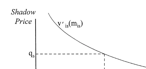
receive a quantity of services, mi s determined by:
ÕXi s
Ž
mi s.
sq .sŽ .
3Let the amount of spending determined by the equation above be denoted by
Ž . Ž .
mi s q . Note that 3 is simply a demand function, relating the quantity ofs
Ž .
services to the shadow price in a managed care plan. See Fig. 1.
The use of a shadow price as a description of rationing in managed care permits
a natural interpretation of the division of responsibility between the A
manage-mentB of a plan, presumably most interested in profits, and the AcliniciansB in a
plan who face the patients. Cost-conscious management allocates a budget or a physical capacity for a service. Clinicians working in the service area do the best they can for patients given the budget by rationing care so that care goes to the patients that benefit most. In this environment, management is in effect setting a shadow price for a service through its budget allocation. It is evident in data that individuals with the same disease get different quantities of service. The constant
8
Risk adjustment can be viewed as a tax-subsidiary scheme used to equalize incentives to ration all services equally. This idea is developed in the general case of many services in Glazer and McGuire
Ž2000b ..
9 Ž .
Fig. 1. Determination of spending on service s for individual i.
shadow price assumption is consistent with managed care rationing but with more
care being received by patients whoAneedB it more.10
2.3. Profit and profit maximization
4
Let qs q , q , . . . , q1 2 s be a vector of shadow prices the plan chooses and
Ž . Ž . Ž . Ž .4
m qi s mi1 q , m1 i2 q , . . . , m2 i s qs be the vector of spending individual i
Ž . Ž Ž .. Ž .
gets by joining the plan. Define n qi 'n m q . Expected profit,i i p q , to the
plan will depend on the individuals the plan expects to be members, the revenue the plan gets for enrolling these people, and the costs of each member. Thus,
p
Ž .
q sÝ
n qiŽ .
riyÝ
mi sŽ .
qs ,Ž .
4s i
Ž .
where r is the possibly risk-adjusted revenue the plan receives for individual i.i
Ž .
The plan will choose a vector of shadow prices to maximize expected profit, 4 .
Ž .
Definepi q to be the gain or loss on individual i:
pi
Ž .
q sriyÝ
mi sŽ .
qs .Ž .
5s
Ž
Given this, for one such service s dropping the arguments q and q from alls
.
functions , the condition for profit maximization is:
dp d ni X
s
Ý
ž /
piyn mi i s s0.Ž .
6d qs i d qs
Ž . X
Condition 6 has two parts. Consider the termyn m . If the shadow price q isi i s s
raised, the plan will spend less by mXi s on individual i if he joins the plan. This
10
term is always positive, reflecting the savings the plan can achieve by rationing
Ž .
more stringently. The other term, d nird qspi, may be positive or negative for
any individual. The term d nird qs is always negative, reflecting the fact that
everyone will find the plan somewhat less attractive as q is raised. Thes pi will
be positive or negative, depending on whether the risk-adjusted revenue is above or below the costs the individual will incur given the rationing in the plan. The idea behind competition among managed care plans is that the first term must after summation be negative — the plan by rationing too tightly will lose profitable customers — to balance the plan’s incentive to reduce services to the existing enrollees.
Ž .
To see what 6 implies for various services, we make some substitutions. The change in the probability of joining can be written as the product of two derivatives:
d ni d n di Õi s
s .
Ž .
7d qs dÕi s d qs
Ž . X
Ž . Ž . X
From 2 , d nirdÕi s is simply Fi, and from 1 and 3 , dÕi srd qs is q m .s i s
Assuming that the elasticity of demand for service s is the same for all individuals
for every q , and denoting this elasticity by e , we get:s s
e ms i s X
mi ss ,
Ž .
8qs
for every i. Note that the assumption that for every shadow price q the elasticitys
of demand for service s is the same for all individuals does not imply, of course, that all individuals have the same demand curve for that service. It only implies
that demand curves of different individuals, for a certain services, areAhorizontal
multiplicationsBof someAbasicB demand function for the service. Individuals will
differ in their relative demands. One interpretation of this assumption, as in Glazer
Ž .
and McGuire 2000a , is that given someone is sick, a common function describes valuation of a service, but people differ in the probability that they become ill.
X
Ž . Ž .
Substituting for mi s from 8 , we can rewrite 6 as:
n e mi s i s X
F e m p y s0.
Ž .
9Ý
i s i s iqs
i
Ž .
Multiplying through by qsres and summing the terms separately,
q FX
m p y n m s0,
Ý
Ý
s i i s i i i s
i i
or
n m
Ý
i i si
qss X .
Ž
10.
F m p
Ý
i i s iŽ .
From 10 we can make some observations about q in profit maximization.s
Ž .
The numerator of 10 reflects the incentive the plan has to save money on its
expected enrollees. The greater is the numerator, the larger will be q . Thes
denominator describes the expected gains a plan sacrifices by losing enrollees. The
denominator contains a product mi spi weighted by the change in enrollment
probability, FXi. Some enrollees will be profitable, with pi)0 given the risk
adjustment formula in use, and some will be unprofitable, with pi-0. The
association between these gains and losses and spending will determine the value of the denominator.
Ž .
For any service provided in profit maximization, the denominator of 10 must be positive, implying that in profit maximization, provision of all services on average attracts profitable enrollees. This observation echoes a conclusion from the health care payment literature where under prospective payment systems, the enrollment response, or more generally, demand response, induces a provider to
Ž . Ž .
supply a noncontractible input corresponding here to q . See Rogerson 1994 ,s
Ž . Ž .
Ma 1995 , or Ma and McGuire 1997 . Creating profits on the margin in this way
to induce firmAeffortB is inconsistent with zero profitability unless marginal costs
are less than average costs or the payer uses a two-part tariff of some kind to reimburse the provider.
In a first-best allocation, a payer or regulator would induce the plan to set
qss1, leading to an equality between the marginal benefit of spending on a
Ž .
service and its marginal cost. Eq. 10 shows how a payer could do this for this
one service by manipulating the payment r . For a given level of payment r , if qi i s
were too high, for example, the payer could simply increase r by some factor,i
Ž .
paying more for every potential enrollee. That would raise the denominator of 10 and induce more spending. In the one service case, risk adjustment is not necessary, simply paying more for all enrollees will do. It is only if a plan manipulates quality in more than one dimension of quality that risk adjustment of
premiums paid to the plan has a role in countering selection incentives.11
2.4. Uncertainty
So far we have assumed that each individual i knows with certainty his
Ž .
valuation of each of the s services Õi s mi s , and, hence, given some q, the dollar
amount of the different services that will be provided to him upon joining the plan. In order to make our model more realistic and to prepare for empirical application, we shall now allow for each individual to be uncertain about his future demands for the different services. Let us suppose that each individual has a set of prior
11
Risk adjustment might also need to deal with individual-specific discrimination, such as, in the
Ž .
beliefs about his possible health care demands, and that the plan shares these beliefs.
Let T denote the set of possible health states of each individual and let t denote
Ž . Ž . Ž .4
an element of T. Let zts Õt1 mt1 ,Õt 2 mt 2 , . . . ,Õt s mt s denote the vector of S
valuation functions for the S services, if the health state is realized to be t. We
Ž .
assume that for each t and s,Õt s satisfies the properties discussed earlier.
Each individual i is uncertain about his health state t, but has some prior
Ž . 12
distribution beliefs f over the set of possible states.i Let x be some random
˜
tvariable, the value of which depends on the state t, and let f be a distribution
w x
function defined over T. Let E xf
˜
t denote the expected value of x with respect˜
tto the distribution f.
The modified model has three moves: first, the plan chooses its level of shadow
Ž .
prices qs q , q , . . . , q , second, the individual chooses whether or not to join1 2 s
Ž .
the plan in a manner studied below , and finally the individual’s health state is realized and services are provided.
For a given shadow price q and a valuation functions Õt s, the plan’s
expendi-Ž .
tures on this individual on service s will be mt s q , given by:s
ÕXt s
Ž
mt sŽ .
qs.
sq .sLetzt
Ž .
q sÝ
Õt sŽ
mt sŽ .
qs.
s
w Ž .x
The individual’s expected utility is: mqEf zt q .
Let u denote the individual’s utility if his health state is t and he chooses thet
w x
next best plan. Thus, E uf t is the individual’s expected utility if he chooses the
alternative plan.
We assume no asymmetry of information between the plan and the individual regarding the individual’s health state. Thus, the plan knows the individual’s prior
beliefs, f, about his future health state.13 The plan, however, does not know the
Ž .
true value of m, although it holds beliefsF m about its cumulative distribution.
12
To use conventional terminology, individual i’s prior beliefs, f , can be thought of as thei
individual’sAtype.BAs will be discussed in Section 3, one can make different assumptions about how
Ž
an individual’s prior beliefs are formed. Under some of these assumptions e.g., beliefs are on the basis
.
ofAageB andAsexB only , several individuals may have the same prior beliefs, and hence be of the sameAtype.B Thereafter, we will continue using the terminologyAindividual iB, but one can think of this asAindividual of type i.B
13
A plan imposing shadow price q gauges the individual’s likelihood of joining the plan as:
X nf
Ž .
q s1yFŽ
Ef utyÕ˜
tŽ .
q.
.Ž .
2 yielding an expected profit on the individual of:X
pf
Ž .
q snfŽ .
qž
ryEfÝ
m˜
t sŽ .
qs/
.Ž .
5s
The plan chooses each q to maximize expected profit. To find profit-maximizing
values of q, we differentiate the above with respect to qX:
s
dpf
Ž .
q X X X X XX
w
Xx
sF Ef Õ
˜ ˜
t smt sž
ryEfÝ
m˜
t s/
yn Ef f mt sŽ .
6X
d qs s
X X
Ž .
Using the fact that Õt ssq for all t, and assuming that ms t ss e ms t srqs for all t,
Ž X
.
we get that the right-hand side of Eq. 6 becomes:
n mf
ˆ
X
X X
w x
es
ž
F mˆ
sž
ryÝ
mˆ
/
y/
, where mˆ
sEf m .ˆ
X
qs
s
We can now show how the plan chooses its profit maximizing shadow prices in this case. Assume a population of N individuals. Each individual i has some prior
beliefs f over the set of possible health states. Restoring the subscript i to Eq.i
Ž X
. Ž X
.
6 , summing Eq. 6 over all i and setting it equal to zero, the profit maximizing
q will be:s
n m
ˆ
Ý
i i si X
qss
Ž
10.
X
X
F m
ˆ
ry mˆ
Ý
i i sž
iÝ
is/
Xi ss1 , . . . , s
w x
where m
ˆ
i ssEf i m˜
t s is individual i’s predicted expenditures on services s, wherethe prediction is with respect to the individual’s prior beliefs about his future
expenditures on service s. Definep
ˆ
isriyÝ
mˆ
is .ss1 , . . . , s
To investigate which shadow prices are set high relative to other shadow prices,
Ž X
. X X
we use Eq. 10 to construct a ratio of q to q where s is some other service.s s
We simplify by abstracting from individual differences in enrollment response by
assuming that FiXsFX. This amounts to saying that an increase in the value of
Ž X
.
plan i increases the likelihood of joining for all individuals equally. Eq. 10 can
now be used to write the ratio of two shadow prices, q and qX. Note that theFX
term cancels out of this expression:
m
ˆ
Xpˆ
n mˆ
Ý
i s iÝ
i i sqs i i Y
s .
Ž
10.
X X
qs
Ý
mˆ ˆ
i spiÝ
n miˆ
i sŽ Y
.
There is no particular reason to expect 10 to be equal for all service pairs unless
the risk adjustment system is so good as to equalize the relative incentives to supply each service.
2.5. The effect of indiÕiduals’ information
Information plays an important role in creating distortions of adverse selection.
Ž .
We are now ready to study how individuals’ information beliefs about their future health care needs affect the plan’s profit maximizing shadow prices. Let
m
ˆ
rÝ
i sÝ
ii i
m
ˆ
ss rsN N
2 2
m
ˆ
ymˆ
Ž
ryr.
Ž
.
Ý
i s sÝ
ii i
)
)
s
ˆ
ss srsN N
m
ˆ
ymˆ
mˆ
Xymˆ
XŽ
ryr.
mˆ
ymˆ
Ž
. Ž
.
Ž
.
Ý
i s s i s sÝ
i i s si i
X
r
ˆ
s , ss rˆ
r ssX
Ns s
ˆ ˆ
s s Ns sˆ
s rˆ
Ms
Ý
mˆ
sss1 , . . . , s
X 14
Ž X
.
and assume that nisn, andFis1 for all i. Eq. 10 can then be written as
nm
ˆ
sqss
Ž
11.
2 X X
ˆ
rm
ˆ
qr s sˆ ˆ
y sˆ
q rˆ
s sˆ ˆ
qm Mˆ
Ž
s r s s r.
sÝ
s , s s s s Xž
ss1 , . . . , s/
X
s/s
The effect of an individual’s information on the choice of q enters throughs s
ˆ
s.Suppose, initially, that all individuals are identical in their beliefs about their
health care needs of all services for the coming period. In such a case, s
ˆ
ss0 forˆ
Ž .
all s and qss nrryM for all s. Thus, in this case all shadow prices are the
same and no distortion occurs. This result is independent of the risk adjustment system and of correlation of predicted spending for different illnesses.
Suppose, now, that individuals have some information that makes them differ from each other with respect to their beliefs about their need of some service s. In
such a case,s
ˆ
s)0. Suppose that there is no risk adjustment, so risr. We can seethat the more heterogeneous are individuals with respect to their m , the larger
ˆ
i swill bes
ˆ
s and the higher will be the shadow price q . This is the standard adverses14
selection result. The better the information that individuals have about their future needs, the bigger will be the distortion created by the plan in order to attract the profitable individuals.
The effect of correlation among spending on different services on the shadow
Ž . X
price can also be observed in 11 . If needs are not at all correlated, then r
ˆ
s, ss0and the only effect on the shadow price comes from individuals’ information s
ˆ
s.If, however, needs are correlated, r
ˆ
X)0 and the larger rˆ
X the higher will bes, s s, s
the shadow price of services s and sX.
Ž .
As is also evident from 11 , risk adjustment can counter the distortive forces discussed above. The larger is the correlation between predicted spending on
service s and risk adjustment payment, r
ˆ
r , s, the higher will be the denominator ofŽ11 , and the lower the shadow price..
3. Measuring shadow prices: an empirical illustration
In this section we illustrate how to use our measure. As we noted in the
introduction, the data we will use are from anAunmanagedB plan, so the findings
are merely an example of how to implement our framework. In other words, our purpose here is to illustrate how to use presently available data to calculate a distortion index. The elements that feed into incentives to distort, such as predictability of various services, and correlation among use in various categories of service, are likely to be largely common to managed and unmanaged patterns of care. Our use of Medicaid data means that the population is not representative, but our findings are at least suggestive.
Ž .
Recall from 11 that the profit maximizing shadow prices depend on the individuals’ expectations regarding their future health needs. Therefore, the empir-ical building blocks for measuring shadow prices are the expected spending of individuals by service class and the correlation of expected spending across services under differing information assumptions. Our main strategy here is aimed at obtaining estimates of future spending, conditional on the information assump-tions, which minimize the forecast error. The performance of a number of estimation strategies for health care spending data has been assessed over the past
Ž . Ž .
15 years. Duan et al. 1983, 1984 and Manning et al. 1981 contend that two-part models minimize mean forecast errors under distributional assumptions commonly exhibited by health spending data. Two-part models consist of one equation,
typically a logit, for the yesrno decision about use, and a second equation,
typically estimated by OLS, describing the extent of use, given some use. We use a two-part model for estimation under differing information assumptions. An
Ainformational assumptionB means, operationally, which covariates to include in
Ž .
3.1. Data
The data are health claims and enrollment files from the Michigan Medicaid program for the years 1991–1993. We chose a subset of the data for application of our model. It is therefore important to highlight that the data we use consists
Ž .
largely of spending by poor women 90% ; thus, calculated shadow prices may differ from those for other populations. The sample consists of individual adults who were eligible for Medicaid in 1991 through the Aid to Families with
Ž .
Dependent Children AFDC program, and who were continuously enrolled in this or another Medicaid program through the end of 1993. We excluded individuals who joined an HMO during the study time-period. The resulting sample consisted of 16,131 individuals, with a mean age of 32 years.
3.2. Defining serÕices
There are a variety of approaches one could take to identifying Aservices,B
ranging from very specific treatments, such as angioplasty, to groups of treatments which would be associated with an illness, such as care for hypertension. In this
paper we define a AserviceB as all the treatments received in connection with
Ž .
certain diagnostic classifications. We identify nine classes of services: 1 birth
Ž . Ž . Ž . Ž .
related, 2 cancer care, 3 gastrointestinal problems, 4 heart care, 5
hyper-Ž . Ž . Ž .
tension, 6 injuriesrpoisonings, 7 mental healthrsubstance abuse, 8
muscu-Ž .
loskeletal problems, and 9 an Aall other category.B Each of the services is
defined by a grouping of ICD-9-CM diagnostic codes.15 We chose groups of
conditions according to several criteria. At least 7.5% of the population was treated for each condition in a year. We included conditions that were a mix of
Ž . Ž
chronic cancer, hypertension, mental health care and acute conditions
gastro-.
intestinal, injuries, and birth-related . Treatments for some conditions are likely to be expensive, some much less so. Some treatments for included conditions are arguably quite predictable, such as birth-related spending, while others might be considered more random, such as injuries and poisonings. We classify all health care claims according to the primary diagnosis attached to the claim.
3.3. Patterns of spending
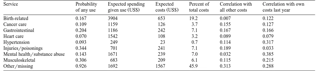
Table 1 describes patterns of utilization and spending for the sample in 1993. The sixth and seventh columns of Table 1 indicate some of the key elements of the
Ž .
formula for shadow prices 11 . The sixth column reports the intertemporal
correlation between spending on each of our nine service categories and the sum of spending on all other services. None of correlations exceeds 0.20, with the
15
()
Frank
et
al.
r
Journal
of
Health
Economics
19
2000
829
–
854
[image:17.842.78.605.164.283.2]845
Table 1
Use and cost in Michigan medicaid AFDC 1993
Service Probability Expected spending Expected Percent of Correlation with Correlation with own
Ž . Ž .
of any use given use US$ costs US$ total costs all other costs costs last year
Birth-related 0.167 3904 653 19.2 0.007 0.122
Cancer care 0.109 1159 126 3.7 0.155 0.127
Gastrointestinal 0.204 1186 242 7.1 0.167 0.166
Heart care 0.070 1542 108 3.2 0.089 0.079
Hypertension 0.093 249 23 0.7 0.114 0.317
Injuriesrpoisonings 0.344 701 241 7.1 0.189 0.033
Mental healthrsubstance abuse 0.143 1671 239 7.0 0.032 0.385
Musculoskeletal 0.306 683 209 6.1 0.115 0.215
exception of theAotherB category. Correlation with spending in the previous year for each category is a measure of the persistence of spending, reported in the seventh column. Persistent spending is probably more predictable. Several of the illnesses thought to be more chronic in character, hypertension, mental
healthrsubstance abuse and musculoskeletal conditions, display relatively high
correlations in service-specific spending over time. Mental-health spending has the highest year-to-year correlation.
3.4. Estimation of components of the ratio of shadow prices
3.4.1. Risk-adjusted premiums
We first calculate the premium assuming that a single payment is made for all enrollees. This premium is based on the simple average level of spending across all enrollees and corresponds to a case with no risk adjustments. We next construct
two sets of trueArisk-adjustedB premiums, one based on the Ambulatory
Diagno-Ž . Ž .
sis Group ADG classification system Weiner et al., 1996 and one based on the
Ž .16
DCG classification system Ellis et al., 1996 . In each case we adjusted the
risk-adjusted premium upward to make the marginal profit per enrollee positive on average, as it must be if plans are to be induced to compete for enrollees by
service quality for all services.17 The increase in premium was 50%.
3.4.2. Expected spending
The variable m
ˆ
i s is the expected level of spending by each individual for eachcategory of service. Estimating expected spending requires assumptions about the information available to individuals. The literature reflects a wide range of conceptions of what consumers might know about their health risks. Newhouse
Ž1989. suggests that individuals know some of the information contained in
measurable aspects of health status plus the time invariant-person specific compo-nent of the unobserved factors contributing to variation in health care spending.
Ž .
Welch 1985 makes a similar assumption, referring to aApermanentB component
of health spending that is individual-specific. Welch speculates that individuals might know more than this and be able to forecast use of some acute services such as births and some other illnesses. Some empirical work on plan choice confirms
Ž .
the presence of considerable individual knowledge. Ellis 1985 and Perneger et al.
Ž1995 show that an individual’s historical pattern of spending affects health plan.
choice. Other research points to the fact that individuals appear to select plans on
16
We used publicly available algorithms to implement these risk adjustment systems. The ADG algorithm is the 1997 version of the software provided by Jonathan Weiner at Johns Hopkins University. The HCC algorithm is the 1997 version of the software provided by Randy Ellis of Boston University.
17
Ž
the basis of information not contained in risk adjustment systems Cutler, 1994;
.
Ettner et al., 1998 .
We consider the implications of several informational assumptions. Recall that if individuals can predict nothing, there is no selection problem, so no simulation needs to be done for this case. We start with the assumption that individuals can predict based on age and sex. That is, we assume all individuals predict they will spend the average for a person of their age and sex for each service category. Alternatively, we assume individuals can also use the information contained in prior use. As will be seen shortly, if individuals know all the information contained in prior use, existing risk adjusters cannot cope with the selection-in-duced inefficiencies, and some services would have very high or very low q’s in profit maximization. In the simulations, we therefore equip individuals with some of the information in prior use, 40%, to illustrate the impact of more information. In order to construct these estimates under different information conditions, we estimate a series of two-part models. Each two-part model uses right-hand side variables at their 1991 values to explain service-specific spending in 1992. Variables included in the model correspond to information individuals are as-sumed to be able to use to predict spending. We estimate two sets of regressions, one with age and sex as right-hand variables and one with age, sex, and prior spending. The estimated coefficients from each pair of service specific regressions are then applied to 1992 values of the right hand side variables to generate estimates of expected spending for each individual in 1993.
Ž . Ž .
Following Duan et al. 1983 and Manning et al. 1981 , each two-part model is specified as:
logit Pr Spending on services s
Ž
Ž
)0.
.
isbX1Xiq´i1Ž
12.
X
(
Ž
Spending on services sNspending)0.
isb2Xiq´i2Ž
13.
where i indexes the individual enrollee, X is a vector of individual characteristics
Žeither age, sex, or age, sex, and prior use ,. b is a vector of coefficients to be
Ž . Ž .
estimated and ´ is a random error term. Eq. 12 is a logit regression. Eq. 13 is a
linear regression that estimates the impact of the X ’s on the square root of the level of spending on each service for individuals with positive spending on that service. We chose the square root transformation to deal with skewness in the distribution of spending rather than the more common logarithmic transformation because the smearing estimator for the square root model is less sensitive to
heteroskedasticity than the log transformation.18 The difficulties in retransforming
Ž .
the two-part model have been treated in detail by Manning 1998 and Mullahy
18
Ž .19
1998 . Since this application calls for predicting 1993 spending using 1992 data
and coefficients from the two-part model of 1992 spending on 1991 right side
variables, a Asmearing factorB is taken from the error term of the 1991–1992
regressions. Because we use a square root transformation, the smearing factor is additive as opposed to the multiplicative form in the case of the logarithmic transformation. The resulting empirical analysis consists of a set of 18 regressions for each of the two informational assumptions we make.
3.4.3. Plan enrollment
We assume that competing managed care plans are in a symmetric equilibrium, and the plan therefore enrolls a representative sample of the population. To
Ž .
estimate plan spending on each service, theÝi sn mi i s in the numerator of 10 , we
will simply use the average spending in the sample.
3.5. A welfare index
The welfare loss associated with a set of q’s can be approximated by:
Ls
Ý
0.5Ž
Dqs. Ž
Dms.
Ž
14.
s
where Dq is the absolute value of the discrepancy between the q for service ss
and the second best q, and Dms is the change in spending induced by the
discrepancy in q. For purposes of this analysis we define Dq as the differences
between q and the weighted average q for all service types contained in Table 3.s
Thus, for each service s, we take the expenditure-weighted average q for each
informationrrisk adjustment combination, and computeDq based on that. Sinces
Dq is in percentage terms,s Dm is simplys Dq multiplied by demand elasticity,s
which we assume for simplicity is 0.25 for all services, except for mental health
Ž .
which we set at 0.5, based on Newhouse et al. 1997 .
3.6. Results
We summarize the predictions of the 18 two-part models in Table 2 by reporting the correlations between actual and predicted service specific spending levels. This correlation is negatively and monotonically related to the absolute prediction error of the spending model. As expected, correlations between actual and predicted spending are generally quite low for all services when only age and sex related information is known by consumers. The birth-related correlation
19
Those papers show the sensitivity of expected spending estimates to distributional properties such as heteroskedasticity. The use of a transformation to account for skewness in the spending data necessitates use of theAsmearingB estimator to retransform the predicted values of spending to the
Ž .
Table 2
Correlations between actual and predicted spending with different information assumptions
a
Service Model
Age–sex Age–sex prior spending
Birth-related 0.210 0.216
Cancer care 0.035 0.104
Gastrointestinal 0.031 0.184
Heart care 0.075 0.104
Hypertension 0.055 0.227
Injuriesrpoisonings 0.002 0.014
Mental healthrsubstance abuse 0.019 0.306
Musculoskeletal 0.073 0.178
Otherrmissing 0.052 0.099
a
All correlations are significant at p-0.01.
between actual and predicted spending is, however, relatively large at 0.21
Žprobably a result unique to a Medicaid sample . With prior use included, the.
correlation between predicted and actual spending improves markedly for most services.
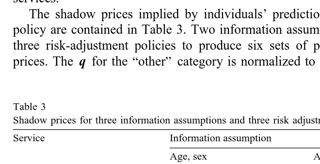
The shadow prices implied by individuals’ predictions and a risk adjustment policy are contained in Table 3. Two information assumptions are combined with three risk-adjustment policies to produce six sets of profit-maximizing shadow
prices. The q for theAotherB category is normalized to 1.00 in all cases, so each
Table 3
Shadow prices for three information assumptions and three risk adjustment systems
Service Information assumption
Age, sex Age, sex 40% of prior use
Risk adjuster Risk adjuster
None ADGs HCCs None ADGs HCCs
Birth-related 1.15 1.25 1.23 0.19 0.35 0.43
Cancer care 0.99 0.98 0.98 0.17 0.28 0.34
Gastrointestinal 0.99 0.99 0.99 0.18 0.29 0.36
Heart care 1.00 0.90 0.89 0.19 0.27 0.33
Hypertension 1.01 0.87 0.87 0.27 0.26 0.28
Injuriesrpoisonings 1.00 1.02 1.02 0.31 0.45 0.52
Mental healthrsubstance abuse 0.99 0.98 0.98 3.73 0.67 0.76
Musculoskeletal 0.97 0.94 0.95 0.18 0.27 0.33
Otherrmissing 1.00 1.00 1.00 1.00 1.00 1.00
Weighted average of q’s 1.03 1.04 1.04 0.82 0.67 0.70
Ž .
Welfare loss % 0.6 1.1 1.0 9.7 3.9 3.6
[image:21.595.52.382.364.534.2]entry in the table needs to be read as the shadow price relative to this numeraire. Begin with the first three columns of results, computed for the assumption that individuals can forecast health costs based only on their own age and sex. The very first column shows the consequences of no risk adjustment with this informational assumption. Individuals cannot forecast very well at all, so the incentives plans have to distort are small, even with no risk adjustment. All estimated q’s are close to 1.00 with the exception of birth-related expenditures. Risk adjustment using ADGs and HCCs magnifies the distortion in the cases of birth-related services, heart care and care for hypertension. The explanation is that people who anticipate using these services are paid for relatively generously in these two risk adjustment formulae.
The welfare loss measure at the bottom of the table corroborates the q results. When there is no risk adjustment and people forecast on age and sex, there is not much distortion, as indicated by the welfare loss as a percentage of spending. Risk adjustment exacerbates the welfare loss, though the magnitude is not high.
The second panel of three columns presents calculated q’s, assuming individu-als can predict spending based on 40% of the information contained in prior spending. Note that with no risk adjustment, mental health and substance abuse services are quite distorted as evidenced by the q of 3.73. Risk adjustment attenuates the distortions, moving all q’s toward unity. Mental health and sub-stance abuse services continue to have the largest service-specific q.
The two risk-adjustment systems studied, ADGs and HCCs, have very similar effects on incentives. For some services, notably birth-related expenditures, risk adjustment improves matters, moving the profit-maximizing q closer to the overall average, but a favorable effect of risk adjustment is not uniform. The incentives to overprovide care for hypertension are exacerbated by risk adjustment. Mental health and substance abuse changes from a service that tends to be underprovided to one much closer to the average with either risk adjustment system. Without risk adjustment, the welfare loss due to selection in the case when individuals know
40% of the information in prior use has risen to almost 10% of spending.20 Risk
adjustment appears to be quite effective, reducing the measured distortion to about
50% of its original magnitude.21A similar analysis could be conducted to examine
how shadow prices change if we were toAcarve-outB any of the service from the
overall insurance contract. The obvious candidate for a carve-out, based on Table 3, is mental health and substance abuse.
20
This is likely to be a conservative measure because of the way we construct elasticity.
21
A next step in this analysis would be to find theAoptimal risk adjustment.BGiven a set of variables
Ž .
available for risk adjusting, Eq. 14 could be minimized with respect to the weights on the risk adjusters. It turns out it is possible to fullyAsolveBthe optimal risk adjustment problem for the services
Ž
if there are enough degrees of freedom in the variables available for risk adjustment Glazer and
. Ž .
As Table 3 shows, the calculations for shadow prices are sensitive to how much information individuals have in making their predictions. When we examined a scenario with individuals knowing as much as 50% of prior use, profit-maximizing
the q’s wentAoff the charts,B signaling that incentives to over and underprovide
are very strong.
4. Conclusion
Health plans paid by capitation have an incentive to distort the quality of services they offer to attract profitable and deter unprofitable enrollees.
Character-izing plans’ rationing as imposing aAshadow priceB on access to care, we show
that the profit maximizing shadow price for each service depends on the dispersion in health costs, how well individuals forecast their health costs, the correlation among use in illness categories, and the risk adjustment system used for payment. We further show how these factors can be combined to form an empirically implementable index that can be used to identify the services that will be most distorted in competition among managed care plans. A simple welfare measure is developed that measures the distortion caused by selection incentives. We apply our ideas to a Medicaid data set to illustrate how to calculate distortion incentives, and we conduct policy analyses of risk adjustment.
From the practical standpoint of health policy, our paper shows how the incentives to distort services depend in a relatively straightforward way on means and correlations among predicted values of health care services in a population. Several interesting findings emerge from the small data set we analyze. The most striking is the importance of individuals’ knowledge and their ability to forecast their health expenses. This factor has been appreciated in abstract terms in earlier writing, but the dramatic effect that information has on incentives has not been empirically demonstrated. According to our preliminary analysis, if people know
Ž
what they are sometimes commonly assumed to know age, sex and prior
.
spending , selection incentives would be very severe. Study of what individuals forecast is a key area of empirical research.
In our models if individuals knowAtoo much,Bsome services are not provided
at all. We therefore analyze hypothetical cases in which individuals are not
allowed to know Atoo much.B Within this limitation, we illustrate how risk
adjustment can be assessed. Two proposed risk adjustment systems have signifi-cant and similar effects in terms of cutting the magnitude of distortion incentives.
Acknowledgements
Research support from the Health Care Financing Administration Cooperative
Ž .
Mental Health NIMH , and grant a23498 from the Robert Wood Johnson
Foundation is gratefully acknowledged. We thank Randy Ellis, Arleen Leibowitz, Joseph Newhouse and participants in the BU-Harvard-MIT Health Economics Seminar for comments on an earlier draft. Pam Berenbaum provided very capable programming and statistical assistance.
References
Baumgardner, J., 1991. The interaction between forms of insurance contract and types of technical
Ž .
change in medical care. RAND Journal of Health Economics 22 1 , 36–53.
Brown, R., Bergeron, J.W., Clement, D.G., 1993. Does managed care work for medicare. Working paper, Mathematica Policy.
Ž .
Cutler, D.M., 1994. A guide to health care reform. Journal of Economic Perspectives 8 3 , 13–29.
Ž .
Cutler, D.M., 1995. Cutting costs and improving health: making reform work. Health Affairs 14 1 , 161–172.
Cutler, D.M., Reber, S., 1998. Paying for health insurance: the trade-off between competition and
Ž .
adverse selection. Quarterly Journal of Economics 113 2 , 433–466.
Cutler, D.M., Zeckhauser, R.J., 2000. The Anatomy of Health insurance. In: Culyer, A., Newhouse, P.
ŽEds. , Handbook of Health Economics. North Holland..
Duan, N., Manning, W.G., Morris, C.N., Newhouse, J.P., 1983. A comparison of alternative models for
Ž .
the demand of medical care. Journal of Business and Economic Statistics 1 2 , 115–126. Duan, N., Manning, W.G., Morris, C.N., Newhouse, J.P., 1984. Choosing between the sample selection
Ž .
model and the multi-part model. Journal of Business and Economic Statistics 2 3 , 283–289. Eggers, P., Prihoda, R., 1982. Pre-enrollment reimbursement patterns of medicare beneficiaries
Ž .
enrolled in at-risk HMOs. Health Care Financing Review 4 1 , 55–74.
Ellis, R.P., 1985. The effect of prior-year health expenditures on health coverage plan choice. In:
Ž .
Scheffler, R.M., Rossiter, L.F. Eds. , Advances in Health Economics and Health Services Research: Biased Selection in Health Care Markets. JAI Press, Greenwich, CT, pp. 149–170. Ellis, R.P., 1998. Creaming, skimping and dumping: provider competition on the intensive and
Ž .
extensive margins. Journal of Health Economics 17 5 , 537–556.
Ellis, R.P., Pope, G.C., Iezzoni, L.I. et al., 1996. Diagnosis-based risk adjustment for medicare
Ž .
capitation payments. Health Care Financing Review 17 3 , 101–128.
Enthoven, A.C., Singer, S.J., 1995. Market-based reform: what to regulate and by whom. Health
Ž .
Affairs 14 1 , 105–119.
Ettner, S.L., Frank, R.G., McGuire, T.G., Newhouse, J.P., Notman, E.H., 1998. Risk adjustment of
Ž .
mental health and substance abuse payments. Inquiry 35 2 , 223–239.
Garfinkel, S.A. et al., 1986. Choice of payment plan in the medicare capitation demonstration. Medical
Ž .
Care 24 7 , 628–640.
Glazer, J., McGuire, T.G., 2000a. Optimal risk adjustment in markets with adverse selection: an application to managed health care. American Economic Review.
Glazer, J., McGuire, T.G., 2000b. Regulating premium payments to managed care plans: minimum variance optimal risk adjustment. Unpublished.
Ž .
Glied, S., 2000. Managed care. In: Culyer, A., Newhouse, J. Eds. , Handbook of Health Economics. North Holland.
Gold, M., Felt, S., 1995. Reconciling practice and theory: challenges in monitoring medicare managed care quality. Health Care Financing Review 16, 85–105.
Holohan, J., Coughlin, T., Ku, L., Lipson, D.J., Rajan, S., 1995. Insuring the poor through Section
Ž .
1115 medicaid waivers. Health Affairs 14 1 , 199–216.
Jensen, G.A., Morrisey, M.A., Gaffney, S.L., Derek, K., 1997. The new dominance of managed care:
Ž .
insurance trends in the 1990s. Health Affairs 16 1 , 125–136.
Keeler, E.B., Newhouse, J.P., Carter, G., 1998. A model of the impact of reimbursement schemes on
Ž .
health plan choice. Journal of Health Economics 17 3 , 297–320.
Keenan, P., Beeuwkes-Buntin, M., McGuire, T., Newhouse, J., 2000. Prevalence of risk adjustment in the U.S., 1998. Unpublished manuscript.
Lerner, A.P., 1934. The concept of monopoly and the measurement of monopoly powers. Review of Economic Studies, 157–175.
Ž .
Luft, H.S., Miller, R.H., 1988. Patient selection and competitive health systems. Health Affairs 7 3 , 97–119.
Ma, C.A., 1995. Health care payment systems: cost and quality incentives. Journal of Economics and
Ž .
Management Strategy 3 1 , 93–112.
Ma, C.A., McGuire, T.G., 1997. Optimal health insurance and provider payment. American Economic
Ž .
Review 87 4 , 685–704.
Manning, W.G., 1998. The logged dependent variable heteroskedasticity and the retransformation
Ž .
problem. Journal of Health Economics 17 3 , 283–296.
Manning, W.G., Morris, C.N., Newhouse, J.P., 1981. A two-part model of the demand for medical
Ž .
care: preliminary results from the health insurance study. In: van der Gaag, J., Perlman, M. Eds. , Health, Economics, and Health Economics. North Holland Publishing, Amsterdam, pp. 103–124. Medicare Payment Advisory Commission, 1998. Report to the Congress: Medicare Payment Policy,
Washington, DC.
Miller, R.H., Luft, H.S., 1997. Does managed care lead to better or worse quality of care? Health
Ž .
Affairs 16 5 , 7–25.
Ž .
Mitchell, P.H., Heinrich, J., Moritz, P., Hinshaw, A.S. Eds. , 1997. Outcome Measures and Care
Ž .
Delivery Systems Conference. Medical Care 35 11 pp. NS1–NS5.
Mullahy, J., 1998. Much ado about two: reconsidering retransformation and the two part model in
Ž .
health econometrics. Journal of Health Economics 17 3 , 247–282.
Netanyahu Commission, August 1990. Report of the State Commission of Inquiry into the Functioning and Efficiency of the Health Care System, Israel.
Newhouse, J.P., 1989. Adjusting capitation rates using objective health measures and prior utilization.
Ž .
Health Care Financing Review 10 3 , 41–54.
Ž .
Newhouse, J.P., 1994. Patients at risk: health reform and risk adjustment. Health Affairs 13 1 , 132–146.
Newhouse, J.P., Buntin, M.J., Chapman, J.D., 1997. Risk adjustment and medicare: taking a closer
Ž .
look. Health Affairs 16 5 , 26–43.
Pauly, M.V., Ramsey, S.D., 1999. Would you like suspenders to go with that belt? An analysis of
Ž .
optimal combinations of cost sharing and managed care. Journal of Health Economics 18 4 . Perneger, T.V., Allaz, A.F., Etter, J.F., Rougemont, A., 1995. Mental health and choice between
Ž .
managed care and indemnity health insurance. American Journal of Psychiatry 52 7 , 1020–1025. Robinson, J.C., Gardner, L.B., Luft, H.S., 1993. Health plan switching and anticipated increased
Ž .
medical care utilization. Medical Care 31 1 , 42–51.
Rogerson, W.P., 1994. Choice of treatment intensities by a nonprofit hospital under prospective
Ž .
pricing. Journal of Economics and Management Strategy 3 1 , 7–52.
Schlesinger, M., Mechanic, D., 1993. Challenges for managed competition from chronic illness. Health Affairs 12, 123–137.
van de Ven, W.P.M.M., Ellis, R., 2000. Risk adjustment in competitive health plan markets. In: Culyer,
Ž .
A., Newhouse, P. Eds. , Handbook of Health Economics. North Holland.
van Vliet, R.C.J.A., van de Ven, W.P.M.M., 1992. Towards a capitation formula for competing health
Ž .
Weiner, J.P., Dobson, A., Maxwell, S.L., Coleman, K., Starfield, B.H., Anderson, G.F., 1996. Risk-adjusted capitation rates using ambulatory and inpatient diagnoses. Health Care Financing
Ž .
Review 17 3 , 77–99.
Welch, W.P., 1985. Medicare capitation payments to HMOs in light of regression toward the mean in
Ž .