arXiv:1709.05585v1 [math.ST] 17 Sep 2017
Fokker-Planck Equations in Large Dimensions∗
Nan Chen†, Andrew J. Majda‡, and Xin T. Tong§
Abstract. This article presents a rigorous analysis for efficient statistically accurate algorithms for solving the Fokker-Planck equations associated with high-dimensional nonlinear turbulent dynamical systems with conditional Gaussian structures. Despite the conditional Gaussianity, these nonlinear systems contain many strong non-Gaussian features such as intermittency and fat-tailed probability density functions (PDFs). The algorithms involve a hybrid strategy that requires only a small number of samples Lto capture both the transient and the equilibrium non-Gaussian PDFs with high accu-racy. Here, a conditional Gaussian mixture in a high-dimensional subspace via an extremely efficient parametric method is combined with a judicious Gaussian kernel density estimation in the remaining low-dimensional subspace. Rigorous analysis shows that the mean integrated squared error in the recovered PDFs in the high-dimensional subspace is bounded by the inverse square root of the de-terminant of the conditional covariance, where the conditional covariance is completely determined by the underlying dynamics and is independent ofL. This is fundamentally different from a direct application of kernel methods to solve the full PDF, where Lneeds to increase exponentially with the dimension of the system and the bandwidth shrinks. A detailed comparison between different methods justifies that the efficient statistically accurate algorithms are able to overcome the curse of dimensionality. It is also shown with mathematical rigour that these algorithms are robust in long time provided that the system is controllable and stochastically stable. Particularly, dynami-cal systems with energy-conserving quadratic nonlinearity as in many geophysidynami-cal and engineering turbulence are proved to have these properties.
Key words. Fokker-Planck equation, high-dimensional non-Gaussian PDFs, hybrid strategy, small sample size, long time persistence
AMS subject classifications. 35Q84, 76F55, 65C05, 37C75, 93B05
1. Introduction. The Fokker-Planck equation is a partial differential equation (PDE) that governs the time evolution of the probability density function (PDF) of a complex
sys-tem with noise [26, 65]. Many complex dynamical systems in geophysical and engineering
turbulence, neuroscience and excitable media have large dimensions and strong nonlinearities, the associated PDFs of which are highly non-Gaussian with intermittency and extreme events
[41, 38]. Predicting the rare and extreme events [15,19,29, 63, 61, 20, 73], quantifying the
uncertainty in the presence of intermittent instabilities [47,6,30,5] and characterizing other
∗Submitted to the editors DATE.
Funding: The research of A.J.M. is partially supported by the Office of Naval Research Grant ONR MURI N00014-16-1-2161 and the Center for Prototype Climate Modeling (CPCM) at New York University Abu Dhabi Research Institute. N.C. is supported as a postdoctoral fellow through A.J.M’s ONR MURI Grant. X.T.T is supported by NUS grant R-146-000-226-133.
†Department of Mathematics and Center for Atmosphere Ocean Science, Courant Institute of Mathematical
Sciences, New York University, New York, NY, USA ([email protected]).
‡Department of Mathematics and Center for Atmosphere Ocean Science, Courant Institute of Mathematical
Sciences, New York University, New York, NY, USA and Center for Prototype Climate Modeling, New York University Abu Dhabi, Saadiyat Island, Abu Dhabi, UAE. ([email protected]).
non-Gaussian features [62, 32] all require solving high-dimensional Fokker-Planck equations with strong non-Gaussian features.
Since there is no general closed-form solution for the Fokker-Planck equation, various nu-merical and approximate approaches have been developed to solve the evolution of the PDF
p(u, t), whereuconsists of the state variables andtis the time. However, traditional numerical
methods such as finite element and finite difference as well as the direct Monte Carlo
simula-tions of the underlying dynamics all suffer from the curse of dimensionality [66,22,64,35,70].
Furthermore, even in the low-dimensional scenarios, substantial computational cost is already required for an accurate estimation of the fat tails of the highly intermittent non-Gaussian PDFs. On the other hand, different methods for solving the partial or the approximate
solu-tions of p(u, t) have been proposed for special dynamical systems. For example, asymptotic
expansion with truncations provides good approximate PDFs associated with the slow varying
variables in non-Gaussian systems with multiscale features [26,55,56,44]. Splitting methods
[23,24], orthogonal functions and tensor decompositions [75, 71,65] are able to provide
rea-sonably good estimations of the steady state PDFs. If the systems are weakly nonlinear with
additive noise, then equivalent linearization method [69, 3] is also frequently used for solving
approximate solutions.
In recent work by two of the authors [14], efficient statistically accurate algorithms have
been developed for solving the Fokker-Planck equation associated with high-dimensional
non-linear turbulent dynamical systems with conditional Gaussian structures [11]. Decomposing
the state variables u into two groups u = (uI,uII) with uI ∈ RNI and uII ∈ RNII. The
conditional Gaussian systems are characterized by the fact that once a single trajectory of
uI(s≤t) is given, uII(t) conditioned on uI(s≤t) becomes a Gaussian process. Despite the
conditional Gaussian structure, the coupled system ofuI anduII is highly nonlinear and it is
able to capture many strong non-Gaussian features such as intermittency and fat-tailed PDFs
that are commonly seen in nature [11]. Note that in most turbulent dynamical systems, the
observed variables uI represent large scale or resolved variables, which usually have only a
small dimension, while the dimension of the unresolved or unobserved variables uII can be
very large [53, 41]. Applications of the conditional Gaussian framework to highly nonlinear
turbulent dynamical systems include modelling and predicting the highly intermittent and
non-Gaussian times series of the Madden-Julian oscillation (MJO) and monsoon [15, 10, 9],
filtering the stochastic skeleton model for the MJO [12], and state estimation of the turbulent
ocean flows from noisy Lagrangian tracers [16, 17, 13]. Other studies that also fit into the
conditional Gaussian framework includes the dynamic stochastic superresolution of sparsely
observed turbulent systems using cheap exactly solvable forecast models [7, 34], stochastic
superparameterization for geophysical turbulent flows [50], physics constrained nonlinear
re-gression models [52, 31], stochastic parameterized extended Kalman filter [28, 27, 6, 8, 36]
and blended particle filters for high-dimensional chaotic systems [54].
The efficient statistically accurate algorithms [14] involve a hybrid strategy that requires
only a small number of samples. In these algorithms, a conditional Gaussian mixture in the
high-dimensional subspace of uII via an extremely efficient parametric method is combined
with a judicious Gaussian kernel density estimation in the low-dimensional subspace ofuI. In
FOKKER-PLANCK EQUATIONS IN LARGE DIMENSIONS 3
full non-Gaussian joint PDF of the system is then given by a Gaussian mixture. One remark-able feature of these efficient hybrid algorithms is that each conditional Gaussian distribution is able to cover a significant portion of the high-dimensional PDF. This guarantees the suffi-ciency of using only a small number of samples, which overcomes the curse of dimensionality.
It has been shown in a stringent set of numerical tests [14] that with an order ofO(100)
sam-ples the mixture distribution has a significant skill in capturing both the statistically steady state and the transient behavior with fat tails of the high-dimensional non-Gaussian PDFs in
up to 6 dimensions while an order ofO(106) samples is required in the Monte Carlo simulation
to reach the same accuracy. In [14], the restriction to 6 dimension of the hybrid method is
not essential but was utilized to allow comprehensive validation of the statistics in the truth model with an instructive simple model.
This article serves as a rigorous analysis for these efficient statistically accurate algorithms.
The main focus here is the accuracy of the recovered PDFs in terms of the sample size L as
well as its dependence on different factors, in particular the dimension of the state variables and the time span. Throughout the article, the mean integrated square error (MISE) is used to quantify the accuracy.
Our first result Theorem 3.1 reveals that the MISE in the recovered high-dimensional
PDFs associated with the unresolved variablesuII is bounded byE(det(RII)−1/2), whereRII
is the conditional covariance of uII given the trajectory of uI. Notably, RII is completely
determined by the underlying dynamical systems and has no dependence on the sample size
L. In contrast, if a direct kernel density method is applied to recover the PDF of uII, then
the bandwidth of the kernel H is scaled as the reciprocal of L to a certain power in order to
minimize the MISE and the resulting MISE is proportional toL−1/NII, which meansLhas to
increase exponentially with NII to guarantee the accuracy in the solution. This indicates the
curse of dimensionality in the direct kernel density estimation and other smoothed versions of Monte Carlo methods. Such a notorious issue is overcome by the efficient statistically accurate
algorithms due to the independence between RII and L in the high-dimensional subspace of
uII. Another significant feature of the efficient statistically accurate algorithms is their long
term persistence, which is affirmed by Theorem 3.7in a rigorous way provided that the joint
process (uI,uII) is controllable and stochastically stable. Theorem 3.7 also supplies a lower
bound of RII using the controllability condition. In addition, Proposition 3.8 demonstrates
that dynamical systems with energy conserving quadratic nonlinear interactions as in most
geophysical and engineering turbulence [41] automatically satisfy all the conditions for the long
time persistence, which justifies the skillful performance of the efficient statistically accurate
algorithms in the numerical tests reported in [14]. Further validations of the controllability and
other theoretical conditions in the algorithms are demonstrated in the numerical simulations at the end of this article.
The remaining of this article is organized as follows. The high-dimensional nonlinear
tur-bulent dynamical systems with conditional Gaussian structures are summarized in section 2,
which is followed by a brief review of the efficient statistically accurate algorithms in [14] for
solving the PDFs of such kind of systems. The main theoretical results are shown insection 3,
where the proofs are included in section 4and the appendix. Insection 5, numerical tests on
a nonlinear triad model and its modified versions are used to validate the theoretical results.
2. Review of the efficient statistically accurate algorithms for solving the PDFs of nonlinear dynamical systems with conditional Gaussian structures.
2.1. High-dimensional conditional Gaussian models with nonlinear and intermittent dynamical features . The general framework of high-dimensional conditional Gaussian models
is given as follows [39,11]:
duI = [A0(t,uI) +A1(t,uI)uII]dt+ΣI(t,uI)dWI(t),
(1a)
duII = [a0(t,uI) +a1(t,uI)uII]dt+ΣII(t,uI)dWII(t),
(1b)
where the state variables are u = (uI,uII) with both uI ∈ RNI and uII ∈ RNII being
mul-tidimensional variables. In (1), A0,A1,a0,a1,ΣI and ΣII are vectors and matrices that are
functions of timetand the state variablesuI, andWI(t) andWII(t) are independent Wiener
processes. Here the noise coefficient matrix ΣI is non-degenerated in order to guarantee the
observability while there is no special requirement for ΣII. The dynamics (1) are named as
conditional Gaussian systems due to the fact that once a single trajectory uI(s) for s≤t is
given, uII(t) conditioned on uI(s) becomes a Gaussian process with mean ¯uII(t) and
covari-anceRII(t), i.e.,
(2) p uII(t)|uI(s≤t)∼ N(¯uII(t),RII(t)).
Despite the conditional Gaussianity, the coupled system (1) remains highly nonlinear and
is able to capture the strong non-Gaussian features as observed in nature [11]. One of the
desirable properties of the conditional Gaussian system (1) is that the conditional distribution
in (2) has the following closed analytical form [39],
(3)
d¯uII(t) =[a0(t,uI) +a1(t,uI)u¯II]dt+ (RIIA∗1(t,uI))(ΣIΣ∗I)−1(t,uI)×
[duI−(A0(t,uI) +A1(t,uI)¯uII)dt], dRII(t) ={a1(t,uI)RII+RIIa∗1(t,uI) + (ΣIIΣ∗II)(t,uI)
−(RIIA∗1(t,uI))(ΣIΣ∗I)−1(t,uI)(RIIA∗1(t,uI))∗ dt.
In most geophysical and engineering turbulent dynamical systems, the nonlinear terms such as the nonlinear advection have quadratic forms and these quadratic nonlinear
interac-tions conserve energy [31,46,52,41,55,56]. The nonlinear interactions allow energy transfer
between different scales that induces intermittent instabilities in the turbulent dynamical systems. Such instabilities are then mitigated by energy-conserving quadratic nonlinear inter-actions that transfer energy back to the linearly stable modes where it is dissipated, resulting in a statistical steady state. Note that the nonlinear turbulent systems without the energy-conserving nonlinear interactions may suffer from non-physical finite-time blow up of statistical
solutions and pathological behavior of the related invariant measure [58]. Mathematically, the
turbulent dynamical systems with energy-conserving quadratic nonlinear interactions have the following abstract forms:
(4) du=−Λu+B(u,u) +F(t)dt+Σ(t,u)dW(t),
where −Λ = L+D. Here, L is a skew-symmetric linear operator that can represent the β
FOKKER-PLANCK EQUATIONS IN LARGE DIMENSIONS 5
representing dissipative processes such as surface drag, radiative damping and viscosity, etc
[67,72,45,74]. The quadratic operator B(u,u) conserves energy by itself so that it satisfies
the following:
(5) u·B(u,u) = 0.
Notably, a rich class of turbulent models with energy-conserving quadratic nonlinear
inter-actions in (4) belongs to the conditional Gaussian systems (1), including the noisy version
of Lorenz 63 model [40], the reduced stochastic climate model [49, 42], the nonlinear triad
model mimicking structural features of low-frequency variability of GCMs with non-Gaussian
features [48], the modified conceptual dynamical model for turbulence [53], and the two-layer
Lorenz 96 model [37]. See [14] and its appendix for a general framework of conditional
Gaus-sian systems with energy-conserving nonlinear interactions as well as concrete examples.
2.2. The efficient statistically accurate algorithms for solving the PDFs of the condi-tional Gaussian systems. Assume the dimension NI of the observed variables is low, while
the dimension NII of the unobserved variables can be high. This is the typical scenario in
most turbulent dynamical systems, where the low-dimensional variables uI represent large
scales or resolved variables while the high-dimensional ones uII stand for the unresolved and
unobserved variables [53,41].
Below, we summarize the procedures of the efficient statistical algorithms developed in
[14]. First, we generateLindependent trajectories from the stochastic dynamical systems (1).
In fact, the only information that is required for these algorithms isLindependent trajectories
of the observed variables, namelyu1I(s≤t), . . . ,uLI(s≤t). Then, different strategies are used
to deal with the observed variables uI and unobserved variablesuII, respectively. The PDF
of uII is estimated via a parametric method that exploits the closed form of the conditional
Gaussian posterior statistics (3),
(6) p(uII(t)) = lim
L→∞ 1
L
L X
i=1
p(uII(t)|uiI(s≤t)).
Note that the limit L → ∞ in (6) (as well as (7) and (9) below) is taken to illustrate the
statistical intuition, while the estimator is the non-asymptotic version. On the other hand, a Gaussian kernel density estimation method is used for solving the PDF of the observed
variables uI,
(7) p uI(t)
= lim
L→∞ 1
L
L X
i=1
KH
uI(t)−uiI(t)
,
where H= H(t) is the bandwidth matrix, and KH(·) is a Gaussian kernel centered at each
sample point with covariance H(t),
(8) KH
uI(t)−uiI(t)
∼ NuiI(t),H(t)
.
The kernel density estimation algorithm here involves a “solve-the-equation plug-in”
ap-proach for optimizing the bandwidth, the idea of which was originally proposed in [4]. The
solve-the-equation approach does not impose any requirement for the profile of the underlying PDF. Therefore, it works for the non-Gaussian cases and the computational cost comes from numerically solving a scalar high order algebraic equation for the optimal bandwidth in order to minimize the asymptotic mean integrated squared error (AMISE) in the estimator.
Fur-thermore, we adopt a diagonal matrix for H. This greatly reduces the computational costs
while remains the results with reasonable accuracy. Note that in the limitL→ ∞, the kernel
density method is simply the Monte Carlo simulation, where the bandwidth shrinks to zero.
Finally, with (6) and (7) in hand, a hybrid method is applied to solve the joint PDF ofuI
and uII through a Gaussian mixture,
(9) p(uI(t),uII(t)) = lim
L→∞ 1
L
L X
i=1
KH(uI(t)−uiI(t))·p(uII(t)|uiI(s≤t))
.
One important features of these algorithms is that the solutions of both the two marginal
distributions in (6) and (7) and the joint distribution in (9) are consistent with those of
solving the Fokker-Planck equation forp(uII(t)), p(uI(t)) and p(uI(t),uII(t)), respectively.
Practically, L∼O(100) is sufficient for the efficient hybrid method (9) to solve the joint
PDF with NI ≤3 and NII ∼10 while an order of O(106) samples is required for solving the
joint PDF using classical Monte Carlo methods to reach the same accuracy for a 6 dimensional
turbulent system [14]. SinceLis only of order O(100), theLindependent trajectoriesu1I(s≤
t), . . . ,uL
I(s≤t) can be obtained by running a Monte Carlo simulation for the coupled system
(1) withLsamples, which is computationally affordable. In addition, the closed form of theL
conditional distributions in (6) can be computed in a parallel way due to their independence,
which further reduces the computational cost. See [14] for more details.
3. Main theoretical results. The rigorous analysis of the efficient statistically accurate
algorithms involving the hybrid strategy (9) is studied in this section. For comparison, the
theoretical results by applying the kernel density estimation method to the full system (1) is
also illustrated. Note that the kernel density estimation is essentially the Monte Carlo
simula-tion whenLis large and therefore it suffers from the curse of dimensionality. Such comparison
facilitates the understanding of the advantages of the efficient algorithm (9) in recovering the
high-dimensional subspace of uII using only a small number of samples. Below, pt(uI,uII)
represents the true PDF while ˜pt(uI,uII) and ˆpt(uI,uII) stand for the recovered PDFs based
on the pure kernel density estimation and the efficient hybrid method (9), respectively.
Kernel density estimation for the joint PDF.
˜
pt(uI,uII) =
1
L
L X
i=1
KH((uI,uII)−(uiI(t),uiII(t))),
(10)
with KH(uI,uII) = (2πH)−
NI+NII
2 exp − 1
2H
NI
X
i=1
c2iu2I,i− 1
2H
NII
X
i=1
c2i+NIu2II,i !
.
FOKKER-PLANCK EQUATIONS IN LARGE DIMENSIONS 7 Hybrid method — kernel density estimation foruI and conditional Gaussian mixture for uII.
ˆ
pt(uI,uII) =
1
L
L X
i=1
KH(uI−uiI(t))p(uII|uiI(s≤t)).
(12)
with KH(uI) = (2πH)−
NI
2 exp − 1
2H
NI
X
i=1
c2iu2I ,i
!
.
(13)
In (11) and (13), we let H = HC as in (9). The scalar H is the scale of the bandwidth
[68,76,77,4] andc2i are the diagonal terms of Csuch thatc2
iH represents the bandwidth in
one direction. In the following, we mostly concern the performance of ˜pt and ˆpt when L is
large.
One standard metric to measure the performance of a density estimator is the mean integrated squared error (MISE). The MISE of the hybrid method, for example, is the average
L2 distance to the true density:
MISE =E
Z
|pt(uI,uII)−pˆt(uI,uII)|2duIduII.
Note that ˆpt relies on the realization of the samples and therefore it is natural to take the
expectation of the distance.
Applying the Bias-Variance decomposition [25] to the MISE yields
(14) MISE =E
Z
|pˆt(uI,uII)−p¯t(uI,uII)|2duIduII
| {z }
Bias
+
Z
|pt(uI,uII)−p¯t(uI,uII)|2duIduII
| {z }
Variance
,
where ¯pt := Epˆt. The variance part comes from the sampling error of the method and the
bias part comes from the usage of the kernel method. See (28) for a direct proof of this
decomposition.
The MISE and its decomposition (14) will be used to understand the performance of the
two density estimation methods in (10) and (12), where the scenarios with a large number
of samples and a large dimension of the variables NII are of particular interest. Main results
are presented below and the rigorous proofs of these results are shown insection 4. Note that
despite quite a few studies of kernel density estimation, especially in the asymptotic limit,
exist in literature [68,76,77, 33, 4], no analysis has been established for the hybrid method
(12). Moreover, the results here are all non-asymptotic, and therefore they hold for arbitrary
choice of bandwidth parameters. This is important in practice, as the bandwidth matrixH(t)
may change with t.
Theorem 3.1. The two parts of MISE in (14) for the hybrid method (12) are bounded:
Here δ is any fixed strictly positive number. E is the statistical average. J(f(uI,uII))denotes the integral R f2(uI,uII)duIduII. The function M(uI,uII) is an upper bound of the third
In a practical scenario, as the sample sizeLincreases, bandwidthHcan decrease, so that both
the variance and bias terms decrease to zero. By takingδclose to zero and ignoring the higher
order term in the bias upper bound, we recover an upper bound similar to the asymptotic
MISE (AMISE) in [76, Eqn. (2.6)], except that our method also consists a random component
of RII(t):
where the two terms on the right hand side represents the variance and bias, respectively. It
is natural to equate the order of these two terms, that is lettingLH−12NI ∼O(H2). This leads
to the common choice of the bandwidth [33]
(18) H ∼OL−
2 4+NI
and consequentially MISE∼OL−
4 4+NI
.
Notably, the variance part of MISE in (17) depends on uII through E
p
det(πRII(t))
−1
,
which indicates that the hybrid method in (12) performs better with a larger RII(t). This
is consistent with the intuition that a large RII(t) corresponds to a conditional distribution
N(¯uII(t),RII(t)) with a wide band that is able to recover a sufficient portion of the PDF.
3.2. Comparison between the two density estimators. Theorem 3.1already reveals the
advantage of the hybrid method (12) over the the direct kernel density method (10). For a
qualitative comparison of the two methods, we can view the latter as a trivial application of
the hybrid method by taking u′I = (uI,uII) andu′II =∅, and therefore u′II is trivially linear
conditioned on u′
I. A direct application ofTheorem 3.1leads to
FOKKER-PLANCK EQUATIONS IN LARGE DIMENSIONS 9
where Mf ≥ M is the upper bound for third order directional derivative in RNI+NII of pt.
Similar results in the asymptotic setting can be found in [76].
If we use the same bandwidthH and sample sizeLin both method, Comparing (19) with
(15), we find that
˜
pt Bias bound≥pˆt Bias bound,
and moreover
˜
pt Variance bound
ˆ
pt Variance bound
= H
−NII 2 QNII
i=1ci+NI
Epdet(RII(t))
−1.
Practically, a large L is chosen to guarantee the accuracy of the recovered PDFs, which
corresponds to a small bandwidthH. Then the variance part of the direct kernel method is
several magnitudes larger than that of hybrid method, especially when the dimension NII is
high.
As discussed above, one would optimize the choice of H such that the two quantities in
(19) are of the same order, which leads to the scaling H ∼ OL−
2 4+NI+NII
, and also the
overall MISE ∼ OL−
4
4+NI+NII, However, This is much worse than the MISE associated
with the conditional Gaussian method (18) whenNII is large. Alternatively, if one wants the
performance of the direct kernel method to be the same as the conditional Gaussian one (18),
then the sample size needs to increase to Le = L
4+NI+NII
4+NI , which can be many magnitudes
larger than L.
In conclusion, direct application of the kernel method suffers from the curse of
dimension-ality. This is due to the fact that the variance scales with the bandwidth as H−NI+2NII, and
therefore one needs to increase sample size exponentially with the dimension in order to have
a small bandwidth that guarantees the accuracy of the recovered PDFs. However, whenH is
small, the kernel density method approximates the standard Monte Carlo simulation, which suffers from the curse of dimensionality. On the other hand, the hybrid method resolves this
issue by estimating the uII part using a parametric method where the bandwidth (or the
covariance) does not depend onL. Therefore, the performance of the hybrid method (12) can
be much superior than the direct kernel method (10) when NII is large.
3.3. Marginal distribution of uII(t). There are scenarios where the focus is only on
es-timating the density of uII(t). Again, both methods can be applied here. The direct kernel
method (10) results in the estimation of the marginal density
(20)
˜
pt(uII) :=
1
L
L X
i=1
KH(uII−uiII(t)), KH(uII) = (2πH)−
NII
2 exp − 1
2H
NII
X
i=1
c2i+N
Iu
2
II,i
!
.
On the other hand, the hybrid method (12) simply becomes a conditional Gaussian mixture
method which contains no kernel density estimation
(21) pˆt(uII) :=
1
L
L X
i=1
It is straightforward to check these density estimators are the marginal PDFs of the joint
distributions in (10) and (12).
Since there is no kernel involved for the conditional Gaussian method in (21), the MISE
has a simple bound without the bias part:
Proposition 3.2. The marginal MISE of the conditional Gaussian estimator in (21) is bounded as
Following the derivation of (19), the MISE of the direct kernel method in (20) is given by
˜ The hybrid method with the conditional Gaussian mixture is clearly superior for marginal
density estimation, as its MISE (22) is essentially O(L−1), and the bandwidth H has no
dependence on L.
3.4. Fixed subspace. In many scenarios, only a part ofuII is of practical interest. To this
end, we consider hereuPII =PuII, whereP:RNII 7→RN
P
II maps uII onto a lower dimensional
subspace. Below, we study the estimation of the density pP
t(uI,uPII) of (uI(t),uPII(t)) using
the hybrid method.
It is straightforward to show the conditional distribution of uPII(t) given uI(s≤t) follows
the Gaussian density p(uPII|uI(s≤t)) of the following form
FollowingTheorem 3.1, we can show that
Corollary 3.3. Under the same assumption as in Theorem 3.1, the MISE decomposition of
ˆ
pPt has the following two bounds
FOKKER-PLANCK EQUATIONS IN LARGE DIMENSIONS 11 where MP is a upper bound of third order derivative of pP
t in uI, as in (16).
Notably, the variance term depends only on Epdet(πPRII(t)P∗)
−1
, where PRII(t)P∗ is
a NP
II ×NIIP matrix that is independent of the components complementary to uPII(t). In
other words, the performance of the hybrid estimator on a certain part of the components
is independent of the other components. This is particularly useful when NIIP is small. Note
that such a property also holds for the direct kernel method but in practice the kernel method
works only for the case whenNII is small.
3.5. Controllability and a lower bound ofRII. According toTheorem 3.1,RII(t) controls
the sampling variance term in the MISE. Therefore, it is desirable to derive a lower bound
for RII(t). Note that in the conditional Gaussian system (1), uI can be interpreted as an
observation ofuII, andp(uII|uI(s≤t)) is essentially the optimal Kalman filter with covariance
RII(t). Therefore, a lower bound of RII(t) can be guaranteed by the controllability of the
associated signal-observation system. In short, the controllability condition ensures the noise in the system is regular enough such that the optimal filter is not accurate to a singular degree in any component. More discussions on the controllability of Kalman filters can be found in
[18, 21, 51]. A recent work [2] has summarized some of the major results in this area. It
is noteworthy that since the term a1 depends on realization of uI, both the controllability
condition and the lower bounds rely on the realization ofuI.
In our context, a standard way to characterize this notion is the following assumption:
Assumption 3.4. Let Es,t be the matrix flow generated by a1:
d
dtEs,t=a1(t,uI(t))Es,t, Es,s =INII.
Suppose there are constants v >0, m≥0andDc ≥1such that for anyt≥vands∈[t−v, t],
Dc−1INII Es,tE ∗
s,tDcINII, σ
2
II,−INII Σ∗IIΣII σ2II,+INII,
A∗
1(t,uI(t))[ΣIΣ∗I]−1A1(t,uI(t))Dc(|uI(t)|2m+ 1)INII.
Throughout this paper, for two real symmetric matrices A and B, we use AB to indicate that B−A is a positive semi-definite matrix.
While A∗
1(ΣIΣ∗I)−1A1 actually concerns of observability, this bound is very mild. Thus, we
still call Assumption 3.4 the controllability condition.
Proposition 3.5. Suppose NII≥2, and the controllability condition, Assumption 3.4holds, then for any t≥v, RII(t)h−t,v1(uI)INII, where
ht,v(uI) :=v2σ2II,+σ−II2,−D
6 c
v+
Z t
t−v|
uI(r)|2mdr
+v−1DcσII−2,−.
In particular there are constants D1 and D2 such that
EpdetRII(t)
−1
≤D1+D2 Z t
t−vE|
The dependence ofRII(t) onuI(s)|t−v≤s≤t comes from the observational termA1. As is seen
from (3), ifA∗
1(ΣIΣ∗I)−1A1 is large, RII(t) has a large quadratic damping, which can bring
it to a very low level.
In symmetry, an upper bound can be derived if a lower bound of A∗
1(ΣIΣ∗I)−1A1 is
assumed. Furthermore, one can show that the Riccati flow of RII(t) is contractive, so its
dependence on RII(0) is diminishing. Since these results are not directly related to the
performance of the hybrid estimator, we put them in the appendix along with the verification
of Proposition 3.5.
3.6. Long time performance. The simulation of (uiI(t),uiII(t)) can be maintained
con-tinuously, and the conditional Gaussian density estimator (12) can be applied for an online
estimation. One important question to ask is whether the performance, and in particular the MISE, degenerates with time. If this is the case, additional samples are needed to reinforce the estimation, which is however usually difficult to carry out in practice. In this subsection, we show that the conditional Gaussian density estimator has a long time stable performance,
as long as the joint process (uI,uII) is stable and ergodic.
In stochastic analysis, the stability and ergodicity of a process can be guaranteed by energy dissipation and non-degenerate stochastic forcing. For our purpose, we can assume the energy
is dissipative, while the noise is elliptic [57].
Assumption 3.6. Suppose ΣI and ΣII are full rank, and the energy is dissipative with a rate ρ >0 and a constant De
(23) uI·(A0+A1uII) +uII·(a0+a1uII)≤ −ρ(|uI|2+|uII|2) +De.
Theorem 3.7. Under Assumption 3.6, the following hold.
1) The joint density pt converges geometrically to an ergodic measure p∞ with a rate c > 0.
In particular, there is a constant D0 so that
(24) Z pt
p∞
(uI,uII)−1
2
p∞(uI,uII)duIduII ≤D0e−cth|u|2+ 1, p0i
p0
p∞ − 1
2
∞
.
Here h|u|2 + 1, p0i denotes the quantity R(|uI|2 +|uII|2 + 1)p0(uI,uII)duIduII, and kfk∞ denotes the supremum kfk∞= supuI,uII|f(uI,uII)|.
2) Suppose Assumption 3.4 also holds, then for any t >0 and δ >0, NII ≥2, the two parts of the MISE using the hybrid method are bounded by
ˆ
pt Variance≤
Dm,NII,v
LπNI+2NIIH NI
2 QNI
i=1ci
exp(−12ρmNIIt)E|u(0)|mNII +Dm,NII,v
,
ˆ
pt Bias≤
(1 +δ)2
4 H
2J NI
X
i=1
c2i∂u22 I,ip∞(
uI,uII)
!
+(1 +δ)
2
2δ H
3 NI
X
i=1
c2i
!3
J(M∞(uI,uII))
+ 8(1 +δ−1)D0e−cth|u|2+ 1, p0i p0
p∞ −1 2
∞kp∞k∞,
where Dm,NII,v is a constant independent of L andH, and M∞ is a bound for the third order
FOKKER-PLANCK EQUATIONS IN LARGE DIMENSIONS 13
In particular, whent→ ∞, we have
lim sup
t→∞ MISE≤
D2 m,NII,v
LπNI+2NIIH NI
2 QNI
i=1ci
+(1 +δ)
2
4 H
2J NI
X
i=1
c2i∂u22 I,ip∞(
uI,uII)
!
+(1 +δ)
2
2δ H
3 NI
X
i=1
c2i
!3
J(M∞(uI,uII)).
This leads to the same bandwidth and MISE scaling with L, namely:
H ∼OL−
2
4+NI and MISE∼OL−
4 4+NI.
The proof strategy of Theorem 3.7 is straightforward. The first part is simply corollaries of
[60,59, 1]. To reach a bound on the variance part in 2), it suffices to have a lower bound on
EpdetRII(t)
−1
. This can be achieved byProposition 3.5and an energy dissipation argument.
For the bias term, we use the Poincar´e inequality (24) to approximate it with the bias term
at equilibrium.
3.7. Conditional Gaussian turbulent dynamical systems with energy-conserving quadratic nonlinearity. Recall the turbulence modeluwith quadratic energy conserving
non-linear interactions (4)–(5)
du=−Λudt+B(u,u)dt+Fdt+ΣdWt.
The linear damping part provides a uniform dissipation, so for someλ−>0,
u·Λu≥λ−|u|2,
and the nonlinearity termB is quadratic and conserves energy.
In our conditional Gaussian setup, we can decompose the dynamics into the form below
(25) duI = (−ΛI,0uI+BI,0(uI,uI) +FI)dt+ (−ΛI,1+BI,1(uI))uIIdt+ΣIdWI,
duII= (−ΛII,0uI+BII,0(uI,uI) +FII)dt+ (−ΛII,1+BII,1(uI))uIIdt+ΣIIdWII.
The quantities in the brackets naturally correspond to A0,A1,a0 and a1 respectively.
For the damping term Λ, we assume there are constants 0< λ−≤λ+,
(26) λ−INI+NII
ΛI,0 ΛI,1
ΛII,0 ΛII,1
λ+INI+NII.
The energy conservation condition, u·B(u,u) = 0, requires that
(27) uI·BI,0(uI,uI) = 0, uII·BII,1(uI)uII = 0, uI·BI,1(uI)uII+uII·BII,0(uI,uI) = 0.
Proposition 3.8. For the stochastic flow with energy conserving quadratic nonlinearity (25), assume that (26)and (27)hold, andΣIandΣII are of full rank. We have the following results: 1). Assumption 3.6 holds with ρ= 12λ− and De = 2λ−1 (|FI|2+|FII|2).
2). Assumption 3.4 holds with v= 1, m= 1 and
Dc = max
(
1, 2λ+σ
−2
II,−
1−exp(−2λ+)
,σ
2
II,+
2λ−
,2λ2+σI−,−2,2λ
2
BσI−,−2,exp(2λ+)
)
,
where the constants are chosen such that |BII,1(uI)| ≤λB|uI|and σI2,−INI ΣIΣ
∗
I, σ2II,−INII ΣIIΣ ∗
IIσII2,+INII.
The proof ofProposition 3.8is shown inD. The energy conservation property plays an essential
role in verifying the system stability, and
4. Proofs.
4.1. Finite time MISE.
Proof of Theorem 3.1. Denote the one sample path density function:
ˆ
pi(uI,uII) :=KH(uI−uIi(t))p(uII|uiI(s≤t)),
such that the recovered PDF is given by ˆpt(x, y) = L1 PLi=1pˆi(x, y). Consider its average
¯
pt(uI,uII) =EKH(uI−uI(t))p(uII|uiI(s≤t)) =Epˆt(uI,uII).
The true density can be written aspt(uI,uII) =Eδui
I(t)(
uI)p(uII|uiI(s≤t)), since for any test
functionf, the following holds
Z
pt(uI,uII)f(uI,uII)duIduII=Ef(uiI(t),uiII(t))
=EE(f(uiI(t),uIIi (t))|uiI(s≤t)) =E Z
f(uI,uII)δui I(t)(
uI)p(uII|uiI(s≤t))duIduII.
This gives the following result
¯
pt(uI,uII) =EKH(uI−uI(t))p(uII|uiI(s≤t))
=E
Z
du′IKH(uI−u′I)δui I(t)(
u′I)p(uII|uiI(s≤t))
=
Z
du′IKH(uI−u′I)pt(u′I,uII) =:KH∗pt(uI,uII),
where∗denotes the convolution. The Variance-Bias decomposition of the MISE can be made:
E Z
|pˆt(uI,uII)−pt(uI,uII)|2duIduII
=
Z
E|pˆt(uI,uII)−p¯t(uI,uII)|2duIduII+
Z
|p¯t(uI,uII)−pt(uI,uII)|2duIduII
=
Z
var ˆpt(uI,uII)duIduII+
Z
|p¯t(uI,uII)−pt(uI,uII)|2duIduII.
FOKKER-PLANCK EQUATIONS IN LARGE DIMENSIONS 15
Since ¯pt=pt∗KH, so
|p¯t(uI,uII)−pt(uI,uII)|=
Z
KH(uI−uI′)(pt(u′I,uII)−pt(uI,uII))du′I
.
In Lemma A.2, a Taylor expansion on (pt(u′I,uII)−pt(uI,uII)) leads to the following upper
bound for the bias part:
1 +δ
4 H
2J NI
X
i=1
c2i∂u22 I,ipt(
uI,uII)
!
+1 +δ
−1
2 M
2H3 NI
X
i=1
c2i
!3
J(M(uI,uII)), ∀δ >0.
Moreover, in light of the relation ˆpt(uI,uII) = L1 PLi=1pˆi(uI,uII) and the independence of the
density samples ˆpi, we have
Z
var ˆpt(uI,uII)duIduII =
1
L
Z
var ˆpi(uI,uII)duIduII
≤ 1 L
Z
E|pˆi(uI,uII)|2duIduII=
1
LE
Z
|pˆi(uI,uII)|2duIduII.
Note that each ˆpi(x, y) is a Gaussian density with mean (uiI(t),u¯II(t)) and a block diagonal
covariance, where the blocks are given by HC and RII(t), respectively. In Lemma A.1, a
straightforward computation of the L2 norm of a Gaussian density shows that
Z
|pˆi(uI,uII)|2duIduII =
1
qQNI
i=1(πHc2i)det(πRII(t)) .
This leads to the bound of the MISE.
Proof of Proposition 3.2. Denote ˆpi(uII) = p(uII|uiI(s ≤ t)), then following the same
proof as in Theorem 3.1, we have pt(uII) =Epˆi(uII) and ˆpt(uII) = 1
L PL
i=1pˆi(uII). Thus,
Z
|pt(uII)−pˆt(uII)|2duII =
Z
var ˆpt(uII)duII=
1
L
Z
var ˆpi(uII)duII
≤ 1 L
Z
E|pˆi(uII)|2duII =
1
LE
1
p
det(πRII(t)) .
Proof of Corollary 3.3. The proof is identical to the one of Theorem 3.1, as long as one
replaces the densities involving uII to the version for uPII. Therefore it is omitted here.
4.2. Long time result.
Proof of Theorem 3.7. Part 1): The geometric ergodicity, i.e. the following L1
conver-gence, Z
|pt(uI,uII)−p∞(uI,uII)|duIduII ≤D0e−cth|u|2+ 1, p0i,
is a direct result that comes from the framework of [60, 59]. Its equivalence to the Poincar´e
We claim that V(uI,uII) = |uI|2+|uII|2+ 1 is a Lyapunov function of Definition 1.1 in
[1]. Apply the generatorL of the diffusion process
LV = 2uI·(A0+A1uII) + 2uII·(a0+a1uII) + tr(ΣIΣ∗I+ΣIIΣ∗II)
≤ −2ρV + (2ρ+ 2De+ tr(ΣIΣ∗I+ΣIIΣ∗II))≤ −ρV +b1U,
where b= 2ρ+ 2De+ tr(ΣIΣ∗I +ΣIIΣII∗ ), and U = {V(uI,uII)≤b}. The fact that U, and
actually any compact subset, is a petite set can be verified by the same proof of Lemma 3.4 in
[59], since we assumeΣI and ΣII are full rank. The fact the stochastic process is irreducible
can also be verified using the same argument. More details on these arguments are provided
in [57] for more general conditions.
Therefore, applying theorem 1.2 of [1] leads to the L1 convergence above. Theorem 2.1
also applies with f(uI,uII) = p∞p0(uI,uII), which gives (24).
Part 2): We again decompose the MISE into (28).
MISE =
Z
var ˆpt(uI,uII)duIduII+
Z
|p¯t(uI,uII)−pt(uI,uII)|2duIduII.
Following the proof of Theorem 3.1, we have the variance part
Z
varˆpt(uI,uII)duIduII≤E
1
LqQNI
i=1(πHc2i)det(πRII(t)) .
Proposition 3.5leads to E√ 1
det(RII(t)) ≤D1+D2
Rt
t−vE|uI(r)|mNIIdr. To provide a bound for
E|uI(t)|mNII, we verify that any fixed moment |u|2n = (|uI|2 +|uII|2)n is also dissipative.
Applying the generator of the diffusion process yields
L|u(t)|2n= 2n|u|2(n−1)(uI·(A0+A1uII) +uII·(a0+a1uII))
+ntr(Σ∗(|u|2(n−1)I+ 2(n−1)|u|2(n−2)uu∗)Σ)
≤ −2nρ|u|2n+ 2nDe|u|2(n−1)+ 2n2tr(ΣIΣI∗+ΣIIΣ∗II))|u|2(n−1)≤ −nρ|u|2n+Dn,Σ,
whereΣ= [Σ∗I,Σ∗II]∗ and the constant Dn,Σ exists because of Young’s inequality.
Apply Dynkin’s formula for eρnt|u(t)|2n, and combine it with the result above, we have
the following Gronswall’s inequality
(29) E|u(t)|2n≤e−ρntE|u(0)|2n+Dn,Σ
nρ .
To continue, we let n=mNII/2 in (29) and integrate it in time range [t−v, t],
E Z t
t−v|
uI(s)|mNIIds≤vexp(−12ρmNII(t−v))E|u(0)|mNII +
2vDmNII/2,Σ
mNIIρ .
Consequently, there exists a constantDm,NII,v such that
Z
varˆpt(uI,uII)duIduII ≤
Dm,NII,v
LπNI+2NIIH NI
2 QNI
i=1ci
exp(−12ρmNIIt)E|u(0)|mNII +Dm,NII,v
FOKKER-PLANCK EQUATIONS IN LARGE DIMENSIONS 17
For the bias term, R |p¯t(uI,uII)−pt(uI,uII)|2duIduII, we use the Cauchy Schwartz
(a+b+c)2 ≤
1
1 +δ +
δ
2(1 +δ) +
δ
2(1 +δ)
(1 +δ)a2+ 2(1 +δ−1)b2+ 2(1 +δ−1)c2,
with
a=|pt(uI,uII)−p∞(uI,uII)|, b=|p¯t(uI,uII)−p¯∞(uI,uII)|, c=|p∞(uI,uII)−p¯∞(uI,uII)|.
Recall that ¯p∞=KH ∗p∞. Using the same proof as in Theorem 3.1, we have
Z
|p∞(uI,uII)−p¯∞(uI,uII)|2duIduII
≤ 1 +δ
4 H
2R NI
X
i=1
c2i∂2u2 I,ip∞(
uI,uII)
!
+1 +δ
−1
2 H
3 NI
X
i=1
c2i
!3
.
Then apply (24), we have
Z
|pt(uI,uII)−p∞(uI,uII)|2duIduII
≤ kp∞k∞
Z
|pt(uI,uII)−p∞(uI,uII)|2
1
p∞(uI,uII)
duIduII
≤D0e−cth|u|2+ 1, p0i p0
p∞ −1 2
∞kp∞k∞. Next, recall that ¯pt(uI,uII) =
R
KH(u′I)pt(uI−u′I,uII)du′I. Therefore, by Cauchy Schwartz |p¯t(uI,uII)−p¯∞(uI,uII)|2
=
Z
KH(u′I)(pt(uI−u′I,uII)−p∞(uI−uI′,uII))du′I
2
≤
Z
KH(u′I)du′I
Z
(pt(uI−u′I,uII)−p∞(uI−u′I,uII))2KH(u′I)du′I
≤
Z
(pt(uI−u′I,uII)−p∞(uI−u′I,uII))2KH(u′I)du′I.
Consequently,
Z
|p¯t(uI,uII)−p¯∞(uI,uII)|2duIduII
≤
Z
(pt(uI−u′I,uII)−p∞(uI −uI′,uII))2KH(uI′)du′IduIduII
=
Z Z
(pt(uI−u′I,uII)−p∞(uI−u′I,uII))2duIduII
KH(uI−u′I)du′I
=
Z
|pt(uI,uII)−p∞(uI,uII)|2duIduII.
5. Numerical examples. Below, numerical examples are used to support the theoretical
results insection 3. The test model considered here is the followingtriad model [52],
du1
dt =A1u2u3,
(30a)
du2
dt =A2u3u1−d2u2+σ2W˙2,
(30b)
du3
dt =A3u1u2−d3u3+σ3W˙3,
(30c)
where A1+A2 +A3 = 0 represents the energy-conserving nonlinear interactions and d2 >
0, d3 >0 are the damping terms. Note that there is no damping and dissipation in (30a) but
(30) is a hypoelliptic diffusion [57, 59]. Linear stability is satisfied for u2, u3 while there is
only neutral stability of u1. Define E2 =σ22/(2d2) and E3 =σ32/(2d3). It is straightforward
to show that the triad system (30) has a Gaussian invariant measure [43, 52]
peq(u) =Cexp
−1
2
u21 E1
+ u
2 2
E2
+ u
2 3
E3
,
provided that the following condition is satisfied
(31) E1=−A1E2E3(A2E3+A3E2)−1>0.
If the condition in (31) is violated, namely E1 < 0, then the variance in u1 direction will
increase unboundedly and there is no invariant measure for the triad system (30).
Below, two dynamical regimes of the triad model (30) are studied, where the corresponding
parameters are listed in the Table 1. Particularly, the triad system (30) in Regime I has a
Gaussian invariant measure while there is no invariant measure in Regime II due to the fact
that E1 < 0. See Figure 1 for the time evolution of the three marginal variances and one
realization of each variable and [41] for dynamical introduction about such triad models.
Table 1
Parameters of two dynamical regimes of the triad model (30)
A1 A2 A3 d2 d3 σ2 σ3 E2 E3 E1 Var(u1)
Regime I −2.5 1 1.5 1 0.5 1 1 =⇒ 0.5 1 5/11 Bounded
Regime II −0.5 −1 1.5 1 0.5 1 1 0.5 1 −5/3 Unbounded
Denote uI = (u2, u3)T and uII = u1. The triad system (30) belongs to the conditional
Gaussian family (1). Notably, the noise coefficient inuII isΣII = 0, which implies the system
has no controllability. The initial values in the tests below are all given at origin. Here only
the hybrid method (9) is tested and the number of samples is always L= 500.
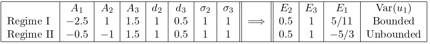
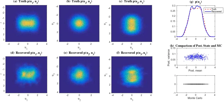
Figure 2 shows the recovered PDF at t = 1 in Regime I of the triad model. Despite an
accurate estimation of the joint PDF of the observed variablesp(u2, u3) as shown in Panel (e),
the recovered PDF of the unobserved variableu1in Panel (f) has quite a few noisy fluctuations
and the recovered joint PDFs p(u1, u2) and p(u3, u1) in Panel (d) and (f) are non-smooth in
FOKKER-PLANCK EQUATIONS IN LARGE DIMENSIONS 19
system, which is consistent with the theoretical discussion insubsection 3.5. In fact, the term
a1 in (1) associated with the triad system (30) is zero. Therefore, according to (3), ΣII = 0
implies the posterior varianceRII =0and the posterior meanu¯II simply follows the sampled
trajectory of uII. In other words, the posterior states from the algorithm are exactly the
Monte Carlo samples, as is validated in Panel (h). The same performance is found in Regime II and thus we omit the figure here.
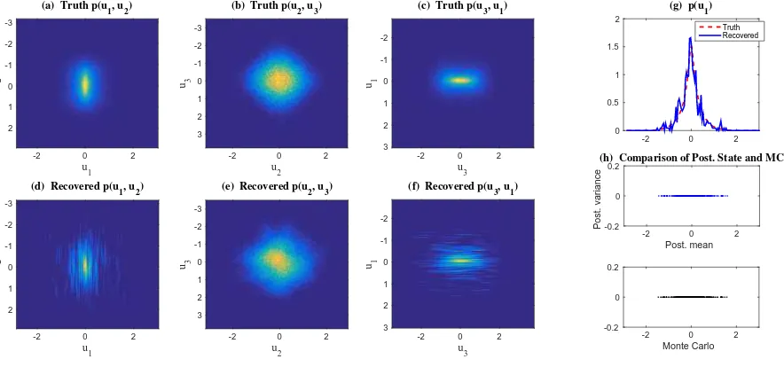
In order to make the triad system have controllability, a small noise is added to (30a) and
the resulting modified triad system is given as follows,
du1
dt =A1u2u3+ǫW˙1,
(32a)
du2
dt =A2u3u1−d2u2+σ2W˙2,
(32b)
du3
dt =A3u1u2−d3u3+σ3W˙3,
(32c)
whereǫis the noise coefficient ofu1 withΣII =ǫin (1). Below we setǫ= 0.1≪σ2 =σ3= 1.
The other parameters in (32) remain the same as those inTable 1.
This extra noise implies the triad system is controllable, which significantly improves the
accuracy of the recovered PDFs. SeeFigure 3for the results in Regime I att= 1. In particular,
Panel (h) ofFigure 3shows that the posterior means are quite different from the Monte Carlo
samples and the posterior variances are no longer zero. It is also shown in Figure 6 that the
recovered PDFs at a long time t = 20 (i.e., statistically steady state) are very close to the
truth with this extra small noise.
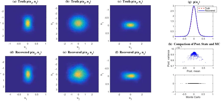
Similarly,Figure 4shows the recovered PDFs of Regime II withǫ= 0.1 att= 1, the error
in which compared with the truth is negligible. Notably, although the amplitude of u1 has
an unbounded growth in this regime due to the fact that E1 <0, the recovered PDFs with
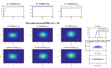
ǫ= 0.1 att= 20 as illustrated inFigure 7remain quite accurate. Next, the performance of the
hybrid algorithm at a very long time in this regime is studied. Figure 5 shows the recovered
PDFs att= 400. Similar toFigure 2, the noisy fluctuations are found in the recovered PDF
of u1. In fact, direct calculations show that the posterior variance RII in (3) is bounded
from above since the unbounded signal u1 does not enter into the evolution of RII, which is
also validated by the numerical simulation in Panel (h). Since the variance of u1 increases
with time, the percentage of the portion covered by each conditional Gaussian distribution decreases in time, which reduces the skill in the recovered PDFs by the conditional Gaussian
mixtures. In Figure 8, we show that by further imposing a damping in the dynamics of u1
of the modified triad model (32) in Regime II, the model then satisfies all the conditions in
Proposition 3.8 and the resulting model has an invariant measure. In such a scenario, the
hybrid algorithm is skillful in both short and long time as is affirmed by Proposition 3.8.
It is also worthwhile pointing out that all the test models in [14], including the noisy
version of Lorenz 63 model [40], the stochastic climate model [49, 42], the nonlinear triad
model mimicking structural features of low-frequency variability of GCMs with non-Gaussian
features [48] and the modified conceptual dynamical model for turbulence [53], all satisfy the
conditions in Proposition 3.8. Therefore, the hybrid algorithm (9) is able to solve the PDFs
0 20 40 60 80 100
(b) Sample Trajectories (a) Variance regimes with parameters inTable 1. (b) Sample trajectories up tot= 1000of the two dynamical regimes. Note the unbounded growth of the amplitude ofu1 in Regime II.
(a) Truth p(u
(d) Recovered p(u 1, u2)
(e) Recovered p(u 2, u3)
(f) Recovered p(u 3, u1)
(h) Comparison of Post. State and MC
FOKKER-PLANCK EQUATIONS IN LARGE DIMENSIONS 21
(d) Recovered p(u 1, u2)
(e) Recovered p(u 2, u3)
(f) Recovered p(u 3, u1)
(h) Comparison of Post. State and MC
Monte Carlo
(d) Recovered p(u 1, u2)
(e) Recovered p(u 2, u3)
(f) Recovered p(u 3, u1)
(h) Comparison of Post. State and MC
Monte Carlo
6. Discussion and Conclusions. This article presents a rigorous analysis for the efficient
statistically accurate algorithms developed in [14], which succeed in solving both the transient
(a) Truth p(u
(d) Recovered p(u 1, u2)
(e) Recovered p(u 2, u3)
(f) Recovered p(u 3, u1)
(h) Comparison of Post. State and MC
Monte Carlo
requires only a small number of samples Lto capture both the transient and the equilibrium
non-Gaussian PDFs with high accuracy.
Theorem 3.1 shows that the MISE in the recovered high-dimensional PDFs associated
with the unresolved variables uII is bounded by E(det(RII)−1/2), where RII is completely
determined by the underlying dynamical systems and it has no dependence on the sample
size L. This is fundamentally different from the direct application of the kernel methods to
recover the PDF of uII, in which the bandwidth of the kernel H is scaled as a reciprocal of
L to a certain power and the resulting MISE is proportional to L−1/NII. This implies the
curse of dimensionality in the kernel density estimation and other smoothed Monte Carlo
methods due to the fact that L has to increase exponentially as NII in order to guarantee
the accuracy in the solution. As is shown in Theorem 3.1, many fewer samples are needed
in the efficient statistically accurate algorithms in order to reach the same accuracy as using
the smoothed Monte Carlo methods, especially with a large NII. Theorem 3.7 affirms the
long term persistence of the efficient statistically accurate algorithms in a rigorous way under
the assumption that the joint process (uI,uII) is controllable and stochastically stable. It
also provides a lower bound of RII using the controllability condition. The validations of
the controllability and other theoretical conditions in the algorithms are demonstrated in the
numerical simulations insection 5. Furthermore,Proposition 3.8illustrates that the turbulent
dynamical systems with quadratic energy conserving nonlinear interactions [41] automatically
satisfy all the conditions for the long time persistence. This justifies the skillful performance
of the efficient statistically accurate algorithms in the numerical tests reported in [14] and
provides important guidelines for future applications.
Appendix. This appendix contains the following information. SectionAstates and proves
Proposi-FOKKER-PLANCK EQUATIONS IN LARGE DIMENSIONS 23
tion 3.5regarding the controllability and observability and Section Cincludes the discussions of the contraction of the Riccati flow. The controllability and long time behavior of the con-ditional Gaussian turbulent dynamical systems with energy-conserving quadratic nonlinearity in Proposition 3.8 are demonstrated in Section D. Finally, extra numerical examples of the
triad model and modified version of the triad model are shown inE.
Appendix A. Two lemmas for Theorem 3.1.
Lemma A.1. Let p(uII) be the PDF of N(a,Σ), its L2 norm is
Proof. Note the Gaussian density has form
p(uII) =
Its square can be decomposed as
p2(uII) =
The second part is the Gaussian density N(a,2Σ), so its integral is one. This concludes our
proof.
Lemma A.2. Suppose pt(uI,uII) has bounded third derivative as (16). Consider filtering it with kernel KH at the uI components, define
and
To continue, we write
|p¯t(uI,uII)−pt(uI,uII)|=
c2i. If we let Z be a random variable following this distribution
FOKKER-PLANCK EQUATIONS IN LARGE DIMENSIONS 25
Finally, by Cauchy Schwartz,
Z
KH(uI−uI′)|uI−u′I|3M(uI+sv,uII)du′Ids
2
≤
Z
KH(uI−u′I)|uI−u′I|6du′Ids
Z
KH(uI −u′I)M2(uI+sv,uII)du′Ids
.
Note again KH is the density ofZ ∼ N(0, HC),
Z
KH(uI−u′I)|u′I−uI|6du′I =E|Z|6 = 15H3
NI
X
i=1
c2i
!3
.
Therefore
Z
duIduII
Z
KH(uI−uI′)|uI−u′I|3M(uI+sv,uII)du′Ids
2
≤15H3
Z
duIduII
Z
KH(uI−u′I)M2(uI+sv,uII)du′Ids
= 15H3
Z
KH(uI−u′I)du′Ids
Z
duIduIIM2(uI+sv,uII)
= 15H3J(M(uI,uII))
Z
KH(uI−u′I)du′Ids= 15H3
NI
X
i=1
c2i
!3
J(M(uI,uII)).
Combine these estimates with 1536 ≤ 12, we have our claimed bound.
Appendix B. Controllability and observability.
Proof of Proposition 3.5. Note that Riccati equation ofRII(t) is given by d
dtRII(t) =a1(t)RII(t) +RII(t)a
∗
1(t) +ΣIIΣ∗II−RII(t)A∗1(t)(ΣIΣ∗I)−1A1(t)RII(t).
In [2], the matrix flow generated by this equation was studied. (In [2], it was termed as
φ(t)(Q)). Define the controllability and observability Gramian [2]:
Cs,t = Z t
s Er,t
ΣIIΣ∗IIEr,t∗ dr.
Os,t = Z t
s
(Er,t∗ )−1A1∗(r,uI(r))[ΣIΣ∗I]−1A1(r,uI(r))Er,t−1.
Define also the following processes:
Ds,t=Cs,t−1 Z t
s E
r,tCs,rA∗1(r,uI(r))[ΣIΣ∗I]−1A1(r,uI(r))Cs,rEr,t∗ dr
Cs,t−1.
Fs,t=Os,t−1 Z t
s
(Er,t∗ )−1Os,rΣIIΣ∗IIOs,rEr,t−1dr
Theorem 4.4 in [2] has shown that
(33) [Ds,t+Cs,t−1]−1 RII(t) O−s,t1+Fs,t,
by applying the comparison principal between the Riccati equation ofRII(t) and the bounds
in (33).
For the purpose of this proposition, we focus only on the left hand side of (33). First we
find bounds for the controllability Gramian. Note that
Cs,t σII2,+
Z t
s Er,tE
∗
r,tdrDc(t−s)σII2,+INII.
Cs,tσ2II,−
Z t
s Er,tE
∗
r,tdrD−c1σ2II,−(t−s)INII.
Then for t−v≤s≤t, apply Assumption 3.4and the bounds above, we have
Ds,tDcCs,t−1 Z t
s
(|uI(r)|2m+ 1)Er,tCs,rCs,rEr,t∗ dr
Cs,t−1
v2σII2,+Dc3C−s,t1
Z t
s
(|uI(r)|2m+ 1)Er,tEr,t∗ dr
Cs,t−1
v2σII2,+Dc4
Z t
s
(|uI(r)|2m+ 1)dr
Cs,t−2
v2σII2,+σII−2,−Dc6
t−s+
Z t
s |
uI(r)|2mdr
INII.
Consequentially, by takings=t−v, we have RII(t)−1ht,v(uI)INII, where
ht,v(uI) :=v2σII2,+σ−II2,−D6c
v+
Z t
t−v|
uI(r)|2mdr
+v−1DcσII−2,−.
In particular, this leads to pdetRII(t)
−1
≤ pdet(ht,v(uI)INII) = hNt,vII/2(uI). Note that for
for positive a, band m≥1, (a+b)m≤2m(am+bm), we have
h
NII 2
t,v (uI)≤2
NII 2
v3σII2,+σ−II2,−D
6
c +v−1DcσII−2,−
NII 2
+ 2N2II
v2σII2,+σII−2,−D
6 c
NII
2 Z t
t−v|
uI(r)|2mdr
NII 2
.
Then applying Holder’s inequality yields
Z t
t−v|
uI(r)|2mdr
NII 2
≤vNII−
2 2
Z t
t−v|
uI(r)|mNIIdr.
FOKKER-PLANCK EQUATIONS IN LARGE DIMENSIONS 27
In symmetry to Proposition 3.5, we can also find an upper bound for RII(t). For that
purpose, let σA,2 −(t)≥0 be a stochastic process that satisfies:
σ2A,−(t)INII A ∗
1(t,uI(t))[ΣIΣ∗I]−1A1(t,uI(t)).
Proposition B.1. Under Assumption 3.4, for t≥v, we have kRII(t)k gv,t(uI), where
gv,t(uI) :=Dc2
v+
Z t
t−v|
uI(r)|2mdr
+vDc5σII2,+
v+
Z t
t−v|
uI(r)|2mdr
2Z t
t−v
σA,2 −(r)dr
−2
.
Note that σ2A,−(t) essentially characterizes how well the observation of uII is made at time
t. It can be zero or close to zero in certain time periods. During such time periods, little
information is provided by the upper bound in Proposition B.1.
Proof of Proposition B.1. We continue our discussion from the end of the proof of Propo-sition 3.5. For t−v≤s≤t, the observability Gramian is bounded by
Os,t= Z t
s
(Er,t∗ )−1A1∗(r,uI(r))[ΣIΣ∗I]−1A1(r,uI(r))Er,t−1
Dc Z t
s
(|uI(r)|2m+ 1)(Er,tEr,t∗ )−1dr
D2c
t−s+
Z t
s |
uI(r)|2mdr
INII.
Likewise, we have
Os,t Z t
s
σA,2 −(r)(Er,tEr,t∗ )−1drDc−1 Z t
s
σA,2 −(r)dr
INII.
Therefore
Fs,t=Os,t−1 Z t
s
(Er,t∗ )−1Os,rΣIIΣ∗IIOs,rEr,t−1dr
Os,t−1
σ2II,+Os,t−1
Z t
s
(Er,t∗ )−1Os,r2 Er,t−1dr
Os,t−1
D2cσ2II,+
v+
Z t
s |
uI(r)|2mdr
2
O−s,t1 Z t
s
(Er,tEr,t∗ )−1dr
O−s,t1
vDc5σII2,+
v+
Z t
s |
uI(r)|2mdr
2Z t
s
σA,2 −(r)dr
−2
In conclusion, by (33) we have RII(t)gv,t(uI)INII, where
gv,t(uI) :=Dc2
v+
Z t
t−v|
uI(r)|2mdr
+vDc5σ2II,+
v+
Z t
t−v|
uI(r)|2mdr
2Z t
t−v
σA,2 −(r)dr
−2
.
Appendix C. Contraction of the Riccati flow. One practical issue in applying the hybrid
method is how to initialize RII(0), asp0(uI,uII) often does not have an explicit form. In fact,
the value of ˆpt has a diminishing dependence on RII(0) as t → ∞. One way to characterize
this is to consider a covariance process R′II(t) that follows
dR′II = [a1R′II+R′IIa∗1+ΣIIΣ∗II−R′IIA∗1(ΣIΣI∗)−1A1R′II]dt.
Here a1 and A1 are the same as the one in (3), but R′II(0) 6= RII(0). In fact, the rescaled
difference between RII(t) andRII(t)′ converges geometrically fast, although the contraction
rate depends on the realization of uI:
Proposition C.1. Under the same assumptions of Proposition B.1, for anyt≥s≥v,
kRII(t)−R′II(t)k ≤
q
kRII(t)kkRII(s)−1kkR′II(t)kkR′II(s)−1k ×exp
−
Z t
s
fv,r(uI)dr
kRII(s)−R′II(s)k,
where k · k denotes the spectral radius, and
fv,t(uI) :=σ2A,−(t)
Dc6
v+
Z t
t−v|
uI(r)|2mdr
+Dc
−1
≥0.
Note that the same lower and upper bounds inProposition 3.5and Proposition B.1 apply to
RII(t) and R′II(t) here, as they are both driven by uI, which is the only thing the bounds
depend on.
Remark C.2. When σA,− is bounded uniformly away from zero and A1 has no dependence on uI, namely m = 1 in Assumption 3.4, then fv,t is bounded away from zero uniformly in time. In this case, one can also show the initialization of u¯II(0) has diminishing influence on pˆt, since a u¯′II(t) process driven by (3) will converge to u¯II(t) even if u¯′II(0) 6= ¯uII(0) [2]. Although in principle the convergence of the mean process should hold in more general scenarios, the convergence rate will have a very involved dependence on the realization of uI(s). Also it is not a significant property for our estimator, and therefore we omitted here.
Proof of Proposition C.1. We continue our discussion from the end of the proof of Propo-sition B.1. In Proposition 3.3 of [2], it is shown that
RII(t)−R′II(t) =Es,t(RII)[RII(s)−R′II(s)]Es,t∗ (R′II).
Here Es,t(RII) is the solution to
d
dtEs,t(RII) = [a1(t,uI(t))−RII(t)A
∗