wulansari et al 2016

(1)

The spillover effects of foreign direct investment on the

_ﬁ

rms

_’

productivity performances

Dyah Wulan Sari1●Noor Aini Khalifah2●Suyanto Suyanto3

Published online: 27 October 2016

Abstract The study aims to examine foreign direct investment spillover effects on thefirms’ productivity per-formances and to examine the most important component of total factor productivity growth in explaining output growth. This study employs a time-varying stochastic frontier approach for firm level panel data of Indonesian manufacturing industry and performs a non-parametric test of the closeness of two distributions. The results demon-strate that foreignfirms achieve higher productivity but less efficient than domesticfirms. Increasing degrees of foreign ownership is negatively related to firms’ productivity but positively related to firms’ efficiency. There are positive horizontal spillover effects of foreign direct investment on the firms’ productivity and efficiency. The backward spil-lovers have positive impact on firm’s efficiency, and the forward spillovers have positive impact on firm’s pro-ductivity. However, there are negative backward spillover effects onfirms’productivity and negative forward spillover effects on firms’ efficiency. Besides that, within the same market technology spillover from FDI are smaller with higher level of labour quality. In the upstream market, the degree of absorptive capacity of suppliers has a negative impact onfirms’productivity but have a positive impact on

reducing inefﬁciency. In the downstream markets, the

greater ability of the buyers to identify, assimilate and exploit knowledge spillovers, the greater the impact on increasing productivity but the lesser the impact on reducing inefficiency. Finally, this studyfinds that all components of productivity; technological progress, technical efficiency change and scale efficiency change significantly contribute in explaining the TFP growth.

Keywords Foreign direct investment spillovers●Efﬁciency●

Productivity ●Manufacturing industry● Indonesia

JEL Classi_ﬁcations D24● F23

1 Introduction

There are many empirical studies that examine productivity gains from foreign direct investment (FDI) that focus solely on technological (or technical) change. They evaluate the FDI spillover effects on the conventional production

func-tion (Aitken and Harrison 1999; Blomström and Sjöholm

1999; Javorcik 2004; Blalock and Gertler 2008; Kohpai-boon 2009). However, theoretical arguments indicate that

productivity gains from FDI can come from efﬁciency

improvement. Superior technology may not only generate technology progress but also advanced managerial expertise and scale-production knowledge that contributes to techni-cal efﬁciency improvement and scale efﬁciency enhance-ment (Kokko and Kravtsova2008; Smeets2008). Thus, the conventional approach of treating productivity gains from FDI as synonymous with technological change tends to understate the real spillover effects of FDI.

* Dyah Wulan Sari

dyah-wulansari@feb.unair.ac.id

1 _{Department of Economics, Department of Economics and}

Business, Airlangga University, Jl. Airlangga No. 4, Surabaya 60286, Indonesia

2

Department of Economics and Management, National University of Malaysia, UKM, Bangi, Selangor 43600, Malaysia

3

(2)

Given the fact that knowledge transfers from foreign firms are not only in the form of advanced technology but also managerial expertise and scale-production knowledge. Hence, a systematic analysis on FDI spillover effects should not only include technological gains but also technical and scale efficiencies. However, some previous studies have only focused on the effect of FDI spillover as a determinant of relative technical efficiency or distance from the frontier. They have investigated the effects of FDI spillover in explaining efficiency differences, either using stochastic

frontier analysis (SFA) (Mastromarco and Ghosh 2009;

Suyanto et al. 2009) or the related non-stochastic of data

envelopment analysis (DEA) (Kravtsova2008). And, very

hardly toﬁnd any studies that have taken into account both

efﬁciency improvement and technological progress as

sources of productivity gains from FDI.

In order to capture the sources of productivity gains that channel through technical change and efficiency enhance-ment, we investigate the effects of FDI spillover in both respects. Therefore, the paper employs SFA forfirm level panel data and includes a set of FDI spillover variables in determining the production frontier and in affecting devia-tions from frontier. Furthermore, the sources of productivity can be decomposed from stochastic frontier estimation into three components; technological change, technical effi -ciency change and scale efficiency change. The total factor productivity (TFP) growth is the summation of those three productivity components. Then, we examine the most important source of total factor productivity growth in explaining output growth using non-parametric test of the closeness of two distributions.

The organization of this paper proceeds as follows: Section 2 provides a literature review of sources of pro-ductivity gains from FDI. Section 3 discusses data sources and variable construction for panel data. It is continued by model specification and estimation techniques in Sect. 4. Section 5 presents the results for model selection and esti-mation, followed by an analysis of empirical results. The summary of findings and policy implications are given in thefinal section.

2 Literature review

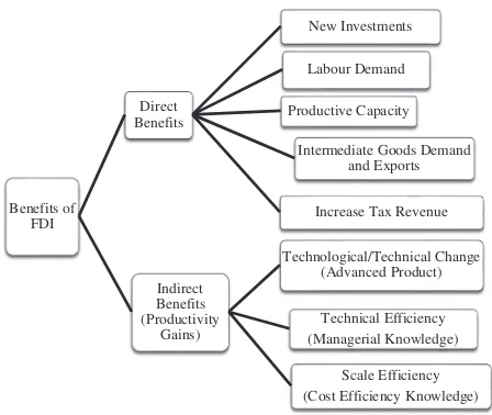
The ability to attract FDI could bring immense benefits to a recipient country. Incoming multinational corporations (MNCs) provide both direct and indirect benefits to the host’s economy. The direct benefits from foreign affiliates can take the form of new investments, productive capacity, labour demand, intermediate goods demand and sometimes exports that stimulate national income or economic growth, provide new opportunity, and increase tax revenue (Takii

2005; Suyanto2010). In addition, the entry of foreignﬁrms

in host country has indirect effects on existing domestic ﬁrms. In the literature, these indirect effects are often called productivity spillovers from FDI (Blomström et al. 2000;

Görg and Strobl 2004; Lipsey and Sjoholm 2005). The

indirect beneﬁts are in the form of knowledge externalities, which are generated through non-market mechanisms to a

recipient economy and the domestic ﬁrms within the

economy. Foreign ﬁrms increase competitive pressure,

which motivates local ﬁrms to improve their productivity. Theoretical arguments indicate that the externalities from inward FDI do not only generate productivity gains to

domestic ﬁrms through technological progress but also

efﬁciency improvement. The ﬁrst form of incoming FDI

indicates that the presence of foreign affiliates may support domesticfirms implementing superior technology to imitate the advanced product which lead to move upward the technological frontier. And the second form imply that substantial inflows of FDI may stimulate domesticfirms to catch-up with the best practice (firms which operate on the frontier) and to reach optimal production scale.

Productivity gains from foreign presence are often regarded synonymously with technological beneﬁts. Firms in a developing country are often lack innovative cap-abilities and typically lag behind foreign afﬁliates. The

introduction of advanced product from foreign ﬁrms may

accelerate the diffusion of new technology in the host country. The presence of advanced products and technolo-gies from foreign affiliates in local markets can inspire and stimulate local innovators to conduct research and devel-opment (R&D) activity. This will support the localfirms for inventions. Hence, positive FDI spillovers to the pro-ductivity growth of domestic firms are reflected in the upward shift of the firms’ production technology (Caves

1971; Glass and Saggi 1999). This argument is consistent within the standard practice of the production function, which assumes that establishments are operated at full efﬁciency and constant return to scale.

(3)

to produce a given amount of output using less input combinations. This technical efﬁciency therefore refers to the ability to avoid waste or slack by producing as much output as input usage allows (Kravtsova and Zelenyuk

2007). Moreover, cost efﬁciency knowledge is also an

important factor for scale efﬁciency. The domestic ﬁrms learn ways to achieve optimal level of production scale,

given with a certain existing resources. Some ﬁrms may

operate under a variable return to scale, so by learn the behavior of foreign firms, domestic firms can increase in returns to scale or scale efficiency advancement (Girma and

Görg 2007). The beneﬁts from encouraging FDI that we

discuss above are illustrated in Fig.1.

Furthermore, the productivity gains from incoming FDI can be transmitted into two broad channels; intra-industry productivity spillovers and inter-industry productivity spil-lovers (Javorcik2004; Girma et al. 2008; Lin et al. 2009; Keller 2009). If the presence of foreign firms generate productivity to domesticfirms in the same industry, these spillovers are considered as intra-industry spillovers or horizontal spillovers. On the other hand, if incoming foreign firms increase productivity of domesticfirms across indus-tries, these spillovers are regarded as inter-industry spil-lovers or vertical spilspil-lovers. The intra-industry spilspil-lovers may occur through three channels of productivity spillovers transmission mechanisms. They are demonstration effect, labour mobility and competition. While, the inter-industry spillovers are channeled through vertical linkages. Vertical technology transfer can arise through both backward (from buyer to supplier) and forward (from supplier to buyer)

linkages. Figure 2 outlines a schematic concept of

pro-ductivity gains transmission from incoming FDI.

The presence of MNC subsidiaries in the domestic market can generate demonstration effects for domestic

ﬁrms in two ways. First, the domestic ﬁrms can adopt

directly from foreign ﬁrm’s technologies through imitation

or reverse engineering (Das 1987; Khalifah and Adam

2009). Local firms can learn how foreign firm affiliates procure, produce, sell, manage, and adapt technology. Obviously, the relevance of this effect increases with the similarity of the good produced by foreignfirms. They can then imitate the behaviour of foreign firms. Second, the domestic firms are stimulated indirectly by new innovation

and R&D (Cheung and Lin 2004). The presence of

advanced products from foreign afﬁliates in host country can encourage and motivate local innovators to do R&D activity which leads to innovation and invention. Therefore, domestic ﬁrms can upgrade the level of their managerial skills and production technology, and may experience increases in productivity.

Another channel for FDI productivity spillovers is rela-ted to labour mobility. The MNCs play a more active role than domesticfirms in educating and training local workers. Through this training, and subsequent work experiences, workers become familiar with foreignfirms’technology and production techniques. The possibility of domestic firms hiring workers who, having previously worked for a foreign firm, know about the technology and are able to implement it in the domesticfirm (Fosfuri et al.2001; Glass and Saggi

2002), resulting in productivity spillovers when the trained

workers move to domestic ﬁrms or establish their own

business (De Mello1997). Nevertheless, it is important to stress a possible negative impact arising through this channel, as MNCs may attract the best workers from domestic firms by offering higher wages. The influence of this labour mobility on the efficiency of local firms is dif-ficult to evaluate as it involves tracking the workers in order to investigate their impact on the productivity of other workers (Saggi 2002). It is not surprising that there is a shortage of detailed studies in relation to this particular aspect.

Furthermore, the competition pressure from FDI is one potentially important determinant of spillovers. The entry of MNCs may lead to greater competition in domestic markets.

Benefits of

Fig. 1 Beneﬁts of foreign direct investment

Productivity

(4)

Foreign firms which enter into a market may increase competition and force localfirms to become more efficient. As long as foreignfirms serve host country markets as well as foreign and domestic products are substitutes, the pre-sence of foreignfirms in a domestic market may increase competition. Competition is an incentive for domesticfirms to utilise existing resources efficiently or even to adopt new technologies. Domesticfirms are then forced to defend their market share by increasing their productivity. However, competition may also restrict the market power of domestic firms. The efficiency of domestic firms may also be nega-tively affected through competition channel. When the profit effects are larger than the efficiency effects, the

competition from foreign ﬁrms may result in negative

spillovers to domesticfirms. Markusen and Venables (1999) argue that the entry of foreign firms to domestic markets reduces domestic firms’ sales, leads to the exit of some domesticfirms, and restores sales of remainingfirms to zero profit level. Aitken and Harrison (1999) present a similar argument but focus on the increasing of average costs in domesticfirms as a factor for the negative spillover effects. The presence of MNCs may imply significant losses of their market shares, forcing them to operate on a less efficient scale, with a consequent increase in their average costs.

A channel of vertical spillovers will exist when the MNC subsidiaries are linked to upstream and downstream indus-tries in host counindus-tries (Rodriguez-Clare 1996; Javorcik

2004; Blalock and Gertler 2008). The domestic ﬁrms in local markets with the MNCs as customers of intermediate inputs may result in backward linkages spillover effect. Meanwhile, MNCs acting as suppliers of intermediate

inputs to domestic ﬁrms may result in forward linkages

spillover effect.

The MNC subsidiaries demand intermediate inputs with a specific standard of quality, which is usually higher than the domestic standard. The MNCs mightfind it profitable to develop local supplier networks and to help improve the performances of these networks by providing information related to sophisticated technology, technical assistance, and other services to local suppliers. In some cases, MNC subsidiaries may also provide technical and managerial training to domestic suppliers to ensure the inputs meet their qualifications. This demand forces domestic suppliers to increase their efficiency and productivity improvement. This channel of productivity spillovers is commonly known as backward linkages.

The MNCs might supply services to local customers that purchase their products for use as inputs. As argued by Javorcik (2008), the entry of MNCs provides new and more suitable inputs for local producers. Access to a greater variety of inputs, especially those with a higher quality, is more likely to increase the efﬁciency and productivity of

ﬁrms in downstream industries. Domestic buyers in

downstream industries may also receive productivity spil-lovers from MNC subsidiaries. The relationship between MNC suppliers and domestic buyers are known as forward linkages.

These links create an opportunity for domestic suppliers or buyers to gain productivity spillovers. This forward spillover together with the backward spillover, sums up to a vertical spillover of FDI in the productivity of domestic suppliers and buyers. This vertical spillover can be seen as a development of an industry by MNC subsidiaries that lead to a development of other related industries.

3 Data sources and variables construction

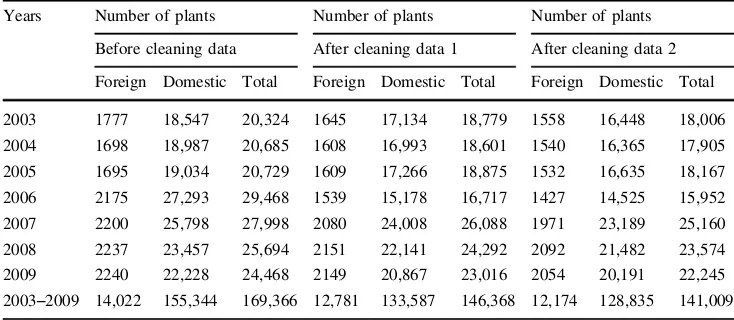
The main data are taken from an annual survey of medium and large manufacturing establishments conducted by the Indonesian Central Board of Statistics (Badan Pusat Sta-tistik or BPS). The survey relies on census and covers all establishments. It is carried out by sending a questionnaire to all large and medium establishments, those are recorded in the directory of establishments compiled by the BPS.1 The medium and large industrial series data are designed to survey all manufacturing establishments employing at least 20 workers in every year. Large establishment is an estab-lishment engaging with more than 99 employees, while medium establishment is an establishment engaging with 20–99 employees. This empirical analysis will use the data from 2003 to 2009.2The numbers of original observations during the periods of study are 169,366 establishments. These observations vary with the year of survey, with the minimum number of 20,324 manufacturing establishments in 2003 and the maximum number of 29,468 establishments in 2006 (Table1).

The main variables used in the production frontier model consist of output and input variables. The output variable is proxy by total gross output. It refers to total value of output produced by a firm in a given year. Capital stock is mea-sured by the replacement value offixed assets. The values of fixed assets contain three asset types: lands and build-ings, machinery and other capital goods, and vehicles. The labour input is measured by the number of employees. The number of employees is used instead of man hours due to the unavailability of the data. Material is the total cost of

1 _Some_ﬁ_{rms may have more than one factory and BPS delivers a}

different questionnaire to the head ofﬁce of everyﬁrm with more than one factory.

2

(5)

domestic and imported raw material used in the production process. While energy is the total expenditure on gasoline, diesel fuel, kerosene, public gas, lubricant and electricity. The output and input material, energy and capital stock are valued in monetary terms and valued in thousand rupiah. Therefore, it is necessary to deﬂate the values output and inputs into real values. Gross output and inputs are deﬂated using a wholesale price index (WPI) published by the BPS at a constant price of 2005. The value of imported material is also controlled using the exchange rate index.

The supplementary data used in this study are input output (I–O) tables. It is used for calculating spillover variables for downstream and upstream industries (back-ward and for(back-ward linkages). The I–O table captures 175 economic sectors and divides manufacturing activity into 90 sectors. BPS provides concordance tables linking the I–O codes to 5-digit ISIC codes. BPS assumes that tech-nology is constant everyﬁve year and that is why BPS only provides data of I–O table every 5 year. During the selected period of the study, it is assumed that technology is con-stant. Hence, all the vertical (backward and forward) lin-kages is estimated by applying an available data of I–O table which were published in year of 2005.3

An unbalanced panel dataset will be used for estimating stochastic production function with inefﬁciency effects.4 There are several adjustment steps to set up an unbalanced

panel data. A few observations are dropped when making consistency checks between industrial codes with interna-tional standard industrial classification (5-digit ISIC).5The data of fixed assets show relatively high variations from year to year. Many establishment report missing value or zero on thosefixed assets. In order to reduce the volatility and impute these missing values, the capital series are regressed against the lagged values of real output to obtain predictions for capital at establishment level. These missing values are calculated following a methodology similar to Vial (2006), Ikhsan (2007) as well as Suyanto and Salim (2013). The capital series are regressed against once lagged values of real output to obtain predictions for capital at establishment level. The predictions are then imputed for establishments which report zero or missing values.6

The dataset are cleaned to minimize noise from non-reporting, misreporting and key-punch error, such as in inputs and foreign share. Some establishments in a given year reported missing values of some inputs, such as material, energy and labour cost. These missing values in these particular variables are eliminated from the observa-tion.7Furthermore, there is obvious typing mistake of raw data in foreign share, for example, foreign share of a ﬁrm for the whole of the selected period is typed as a 100 %, except for a certain year being typed as 0 %, and then the 0 % share is adjusted to 100 %.8During the periods of the

study, more than 2 % domestic ﬁrms changes to foreign

Table 1 The number of foreign and domestic indonesian manufacturing establisments

Years Number of plants Number of plants Number of plants

Before cleaning data After cleaning data 1 After cleaning data 2

Foreign Domestic Total Foreign Domestic Total Foreign Domestic Total

2003 1777 18,547 20,324 1645 17,134 18,779 1558 16,448 18,006 2004 1698 18,987 20,685 1608 16,993 18,601 1540 16,365 17,905 2005 1695 19,034 20,729 1609 17,266 18,875 1532 16,635 18,167 2006 2175 27,293 29,468 1539 15,178 16,717 1427 14,525 15,952 2007 2200 25,798 27,998 2080 24,008 26,088 1971 23,189 25,160 2008 2237 23,457 25,694 2151 22,141 24,292 2092 21,482 23,574 2009 2240 22,228 24,468 2149 20,867 23,016 2054 20,191 22,245 2003–2009 14,022 155,344 169,366 12,781 133,587 146,368 12,174 128,835 141,009 A plant with any share of foreign assets is considered as foreignﬁrm. Cleaning Data 1 is applying material input criteria 1. Cleaning Data 2 is applying material input criteria 2

3 _{Besides that, this study also considers the I}

–O table for the year 2000 for estimating backward and forward linkages for the years 2003 and 2004, while the remaining linkages is estimated using the I–O table for the year 2005.

4

However, this study applies a balanced panel data for calculating output and input growth as well as for decomposing total factor productivity growth into three component sources of productivity. After constructing a balance panel data using observation with material input criteria 1, the numbers of observations in every year are removed to 10,093 ﬁrms. Meanwhile using criteria 2, the numbers of observations become 8705ﬁrms in each year.

5 _For _ﬁ_{rms with same PSID, if they have different ISIC, the most}

dominant ISIC will replace the less dominant ISIC. However, if each

ﬁrm with same PSID has a different ISIC in every year, it is dropped from observations. After this adjustment, the original observations are dropped around 0.13 %.

6

The missing value of ﬁxed assets are around 30.06 % from the original sample, and 70.46 % of them can be estimated.

7

The missing values in material, energy and labour cost are about 0.07 %, 2.87 % and less than 0.01 % from the original sample.

8

(6)

firms and less than 1 % foreignfirms becomes to a domestic firm. The numbers of domestic and foreign establishments in each year are reported in Table1.

When the ratio of material input to gross output is too low or too high, and in some cases the ratio is more than one, which seems to be unreasonable. Hence, the observa-tion is controlled from this implausible sense using material input over gross output criteria. The samples are considered to be excluded from the observations if the value of parti-cular material input in relation to gross output is less than 5 % and higher than 95 %, and we call this material input criteria 1. After this adjustment process, the total observa-tion during the periods of study is 146,368 establishments which are grouped into 34,896 identiﬁcation code (PSID) and 344 industrial classiﬁcations (ISIC). Besides that, this study also accomodates the material input criteria of 10 and 90 %, which we call material input criteria 2 and the number observation reduces to 141,009 establishments which are

classiﬁed into 34,578 PSID and 341 ISIC categories.

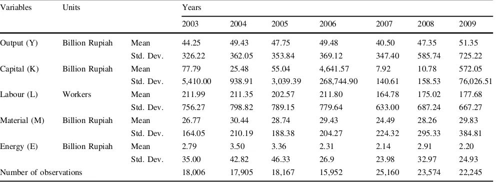
Table2a, b show the main data in each year using these criteria.

The exogenous variables included in the models can be divided into key variables and other exogenous variables. The key variables are set of FDI variables, such as the

dummy variable of foreign ﬁrm (FOR), horizontal

spil-lovers (HSpill), backward spillovers (BSpill) and forward spillovers (FSpill). While, the other variables are openness variables that can be measured by imported input material intensity (Imp) and export intensity (Exp), absorptive capacity variable (Abs), the degree of market competition (HHI) as well asﬁrm size (FSize). All industrial sectors in this study are classiﬁed based on the 5-digit industrial code and all calculations of their values are based on the original observations.

There are some different definitions of foreign owner-ship. According to the different studies, the definition of foreign equity capital varies. Studies by Aswicahyono and Hill (1995), Blomström and Sjöholm (1999), Koirala and Koshal (1999), Ramstetter (1999), Narjoko and Hill (2007), readily accept any positive amount of foreign ownership, while Haddad and Harrison (1993) consider firms with at least 5 % equity owned by foreigners. The IMF (2004) and OECD (2009) definition of foreign firms is defined as an incorporated enterprise in which a foreign investor owns 10 % or more of their equity capital. The IMF and OECD definition is characterized an internationally standard threshold of foreignfirm. Another study, like Djankov and Hoekman (2000) consider the relevant threshold to be 20 %. This study accommodates several thresholds of foreign assets percentages. All joint-venture companies with 5, 10 and 20 % of foreign assets will be considered as foreign firms in the model. Variable of foreign ownership is mea-sured by a dummy variable and it will be defined as:

FORit ¼1 if the share equity of foreign ownershipiat timetis greater than or equals the thresholds:

¼0 if otherwise

ð1Þ

An extension, such as an interacting FORdummy

vari-able with foreign equity share (FSh*FOR) is also included in the model. This interacting variable captures the effect of

higher percentages of foreign ownership on ﬁrms’

pro-ductivity and efﬁciency.

The foreign share of gross output is chosen as a proxy of

horizontal spillover from foreign ﬁrms. As in Javorcik

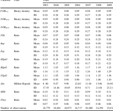
(2004) and Blalock and Gertler (2008), theHSpillvariable Table 2a A statistic summary of the main variables using material input criteria 1

Variables Units Years

2003 2004 2005 2006 2007 2008 2009

Output (Y) Billion Rupiah Mean 45.87 51.39 51.33 52.44 41.11 47.68 51.61

Std. Dev. 341.22 394.55 391.87 408.60 345.90 581.39 713.76

Capital (K) Billion Rupiah Mean 80.25 26.27 54.36 4455.60 8.13 10.78 553.34

Std. Dev. 5336.97 924.39 2982.62 263,000.00 140.18 156.73 74,700.00

Labour (L) Workers Mean 212.50 211.18 204.16 213.50 165.35 174.63 178.42

Std. Dev. 747.62 790.50 788.70 768.72 628.75 683.48 668.09

Material (M) Billion Rupiah Mean 28.36 32.23 32.39 31.94 25.14 28.46 30.25

Std. Dev. 194.04 250.56 251.40 249.03 222.15 291.75 379.20

Energy (E) Billion Rupiah Mean 2.87 3.57 3.52 2.43 2.17 2.87 2.16

Std. Dev. 36.21 44.46 48.40 28.61 24.02 32.51 24.52

Number of observations 18,779 18,601 18,875 16,717 26,088 24,292 23,016

(7)

is the horizontal spillover effects from FDI to domestic ﬁrms’ productivity in the same market. It is calculated as follows:

where HSpilldenotes the horizontal spillover effects, FSh

measures the share offirm’s total equity owned by foreign investors. Y expresses output, subscript i denotes the i-th firm,j describes thej-th industry, i∈j indicates afirm in a given industry andtrepresents time.

FDI can also generate vertical spillovers through the linkage channel. The backward and forward spillover vari-ables here are established according to the I–O table, especially the Leontief inverse matrix which captures both direct and indirect (inter-sectoral) linkages. The measure-ment of vertical linkages in this study will follow Kohpai-boon’s (2009) study. This is different from Javorcik (2004) and Blalock and Gertler (2008) whose vertical linkages proxy captures only the direct linkages.

To do so, inter-industry linkage is constructed based on the Leontief inter-industry accounting framework. Consider an input–output framework in which the import content of each transaction is excluded (non-competitive type):9

X_¼AdX_þYd_þE; Ad_¼½ akl; akl¼Xkl=Xl

ð3Þ

Solving Eq. (3) forX:

X_{¼ ½}I Ad 1_½Yd_þE; ½I Ad 1_¼½ bkl; ð4Þ

where X is column vector of total gross output. Ad is

domestic input output coefﬁcient matrix. [akl] is element of domestic input-output coefﬁcients matrix.10 Yd is column vector of domestic demand on domestically produced

goods. E is column of export demand on domestically

produced goods. [bkl] is the Leontief domestic inverse matrix which captures both direct and indirect (inter-sec-toral) linkages in the measurement process. It shows the total units of output required, directly and indirectly, from all sectors when the demand for the industry’s product rises by one unit.

The variable of backward spillover (BSpill) captures the foreign presence in the upstream industries that are supplied by industry j. The measurement is deﬁned in the following way:

BSpilljt¼ X

k

bklHSpilljt; _ð₅_Þ

wherebklindicates amount of industryk'soutput demanded by an additional unit of industry l's output produced. The

product between each element bkl and its corresponding

degree of foreign presence (bkl*HSpilljt) measures to a certain extent derived demand from foreign presence for industryk'soutput. Hence, the sum of that product indicates total derived demand from foreign ﬁrms for industry k's

output. This indicates the backward linkages from foreign ﬁrms. In Eq. (5), inputs supplied within the industry are not included, because the effects are already captured by hor-izontal spillovers.

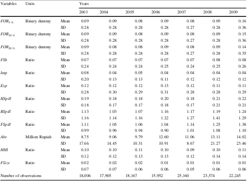
While the FDI effect on suppliers is measured by back-ward spillovers, the FDI effect on buyers is represented by forward spillovers. The forward spillover is calculated in a Table 2b A statistic summary of the main variables using material input criteria 2

2003 2004 2005 2006 2007 2008 2009

Output (Y) Billion Rupiah Mean 44.25 49.43 47.75 49.48 40.50 47.35 51.35

Std. Dev. 326.22 362.05 353.84 369.12 347.40 585.74 725.22 Capital (K) Billion Rupiah Mean 77.79 25.48 55.04 4,641.57 7.92 10.78 572.05

Std. Dev. 5,410.00 938.91 3,039.39 268,744.90 140.61 158.53 76,026.51

Labour (L) Workers Mean 211.99 211.35 202.57 211.80 164.78 175.02 177.68

Std. Dev. 756.27 798.82 789.15 779.64 633.00 687.24 667.27

Material (M) Billion Rupiah Mean 26.77 30.44 28.74 29.43 24.49 28.26 29.83

Std. Dev. 164.05 210.19 188.38 204.27 224.32 295.33 384.81

Energy (E) Billion Rupiah Mean 2.79 3.50 3.36 2.31 2.14 2.91 2.20

Std. Dev. 35.00 42.82 46.33 26.9 23.98 32.97 24.93

Mean=_{arithmetical average, Std. Dev.}=_{standard deviation}

9

There is another type of I–O table in which the import transactions are not excluded from domestic transactions.

10

This coefﬁcients matrix (akl) used by Javorcik (2004) and Blalock

(8)

similar way as backward spillover and excluding outputs produced by foreignfirms for export (Yit−Xit). The purpose of this measure is to capture the potential spillovers from foreign firms to domestic buyers’ productivities. The for-ward spillover is defined as:

FSpilljt¼

where bkl indicates demand for industry k's output to be used as inputs for producing a unit of industry l's output. When multiplying each elementbkl with its corresponding foreign share, this multiplying indicates industrylpurchases its intermediate inputs supplied by foreign plants located in industryk. For the same reason as before, inputs purchased within the industry are excluded. Hence, the sum of that product would reflect a proportion of total intermediate inputs used in industry l supplied by foreign firms, indi-cating forward linkage from foreignfirms.

Having access to leading edge technologies through technology transfers may not itself lead to productivity improvements. An absorptive capacity is a critical factor in firms’ability to catch up with otherfirms at the technological frontier or to shift upward from the technological frontier. Spillovers may not materialize if the technology is not absorbed and utilized efficiently, and then there may be little scope for learning. Therefore, the spillovers effects from FDI do not guarantee to occur automatically, it depends with the capability of the human capital in a receipt country.

Human capital plays a crucial role on absorptive capacity of host industry in which the foreignﬁrms operate. Mas-tromarco and Ghosh (2009) as well as Henry et al. (2009) found that the existing level of human capital is an impor-tant variable for greater technology absorption. The most appropriate indicator to assess human capital on theﬁrms’

productivity and efficiency is the quality of the workers. It represents the skills of workers that affect the productivity and efficiency of thefirm. Unfortunately this, information is not available at firm level data that we use in this study. However, Le and Pomfret (2011) argue since the number of skilled workers are not available, labour costs (including wages and training costs) per worker can be used as a proxy for the human capital stock of thefirm. This is based on the assumption thatfirms with higher average labour costs per worker employ higher skilled labour. Therefore, the labour cost per worker will be used as a proxy for absorptive capacity variable (Absit) in this study. To account for the absorptive capacity in determining the extent of technology spillovers, we interact absorptive capacity variable with the spillover variables. The absorptive capacity may facilitate FDI spillover effects in the Indonesian manufacturing industries. This interaction between technology spillovers from FDI with the absorptive capacity variable may

represent rapid adoption of new technology in the manu-facturing sectors.

Moreover, the openness variables can be determinants that affect theﬁrm’s productivity performance. Technology transfer from international trade provides greater

impor-tance for productivity growth for ﬁrms in developing

countries which have little new technology. Technical progress could be embodied in new materials, intermediate manufactured products, capital equipment are traded on international markets thus allowing countries to import the R&D investments made by others. Keller (2009) suggests that import and export intensities can be a significant channel for transmitting technological knowledge. The importing or exporting plants might receive technology spillovers through their importing or exporting experiences. They might come into contact with foreign technology through their importing or exporting activities, and more likely that they get more access to technology. This raises thefirm technological capacity, which in turn increases the firm productivity. Therefore, both will be included in the model, which import intensity (Impit) is measured by share of imported material and export intensity (Expit) is mea-sured by ratio export to gross output offirmiat time t.

Broadly, ﬁrm’s higher productivity performances can occur as a result of the lower or higher degree of market competition. There are two alternative hypotheses that have been put forward to explain correlation between pro-ductivity performance and competition. On the one hand, higher concentration can be the result of dynamic compe-tition amongﬁrms of differential productivity that removes

less productive ﬁrms from the industry as argued by

Demsetz (1973), Peltzman (1977), Sidak and Teece (2009) as well as Teece (2011). On the other hand, higher con-centration is an inverse measure of static competition that

can protect less productive ﬁrms. This means that

pro-ductivity improvement could be stimulated in the more competitive environment as introduced by Nickell et al. (1997) and Ahn (2002).

(9)

On the other hand, the degree of market competition can affect the level of managers’ and workers’ efforts. Mono-poly rents to monopolisticfirms can be captured by their managers and workers in the form of managerial slack or lack of efforts. Competitive pressure may reduce such slack by giving more incentives to their managers and workers for increasing their efforts and improving efficiency. It can be reasonably expect that product market competition would disciplinefirms into efficient operation. Beside that, com-petition can be also defined in terms of productivity growth through innovations. Productivity gains come from enhan-cing innovations which introduce new and better products, and successful innovations will eventually raise the level and growth rate of productivity.

In the sense of the degree of market competition, theHHI

can be used as a measure of the degree of market compe-tition. Higher values ofHHIindicates greater concentration of sales among producers and thus less competition. The ﬁrst argument suggests that higher value of HHI is asso-ciated with greater productivity, while the latter argument

suggests that higher value ofHHI is associated with lower productivity. The measure of market concentration of industryjat timetcan be calculated as follows:

HHIjt¼ X

n

i_¼1

s2_it; wherei₂j; _ð7Þ

wheres2

i is market share of eachﬁrms.

Theﬁrm size variable (FSize) will also be included in the models. Based on a number of studies such as Moulton (1990) and Kohpaiboon (2009), the FSize in the models controls industry effects, especially when using a sample covering many industries and using aggregation. In this study, theFSizeitis measured by output of theﬁrmidivided by output of the industryjat timet. The summary statistics of exogenous variables discussed above using material input criteria 1 and 2 are presented in Table 3aandb.11 Table 3a A statistical summary

of exogenous variables using material input criteria 1

2003 2004 2005 2006 2007 2008 2009

FOR5 % Binary dummy Mean 0.09 0.09 0.08 0.09 0.08 0.09 0.09

SD 0.28 0.28 0.28 0.29 0.27 0.28 0.29

FSh Ratio Mean 0.07 0.07 0.07 0.08 0.07 0.08 0.08

SD 0.24 0.24 0.24 0.25 0.24 0.25 0.26

Imp Ratio Mean 0.08 0.05 0.05 0.04 0.04 0.04 0.04

SD 0.20 0.13 0.13 0.12 0.12 0.12 0.12

Exp Ratio Mean 0.12 0.12 0.13 0.14 0.12 0.10 0.11

SD 0.29 0.30 0.29 0.31 0.28 0.28 0.29

HSpill Ratio Mean 0.19 0.18 0.18 0.20 0.18 0.21 0.22

SD 0.18 0.17 0.17 0.18 0.17 0.21 0.21

BSpill Ratio Mean 1.13 1.03 1.07 1.16 1.17 1.19 1.25

SD 1.16 1.13 1.15 1.22 1.26 1.40 1.29

FSpill Ratio Mean 1.11 1.05 1.05 1.04 1.14 1.25 1.38

SD 0.99 0.95 0.94 0.90 1.01 1.08 1.10

Abs Million Rupiah Mean 8 .80 9.07 9.90 12.60 11.04 13.06 14.00 SD 17.55 14.46 10.65 10.94 8.71 21.04 23.21

HHI Ratio Mean 0.10 0.10 0.11 0.10 0.09 0.10 0.11

SD 0.12 0.12 0.13 0.13 0.12 0.14 0.14

FSize Ratio Mean 0.02 0.02 0.02 0.01 0.01 0.01 0.01

SD 0.07 0.07 0.06 0.06 0.05 0.06 0.06

Mean=_{arithmetical average, Std. Dev.}=_{standard deviation. Explanations for the subscripts are provided in} footnote 10

11

(10)

4 Model speci

ﬁ

cation and estimation technique

The productivity analysis literature can be divided into two main branches: parametric and non-parametric methods. And, there are two most popular estimation methods which deal with productivity measurement, data envelopment analysis (DEA) and stochastic frontier analysis (SFA). The DEA is representative of the non-parametric method involving a linear programming model. It was originally proposed by Charnes et al. (1978). DEA develops a non-parametric piece-wise surface or frontier which is deter-mined by the most efficient producers over the dataset. It deals with many outputs in a consistent way. It is very flexible in the specification of technology with no particular production function assumption. However, DEA is a deterministic model, because efficiency is measured as the distance to this frontier without involving statistical noise. This makes sensitive to the extreme values or outliers and causes the effect of measurement error to be completely

unpredictable (Van Biesebroeck 2007). Therefore, the

estimated production frontier and efﬁciency measures will be bias.

Most nonparametric methods for measuring efﬁciency

are based on envelopment techniques, such as DEA. Sta-tistical inference based on these estimators is available but, by construction, they are very sensitive to the outliers. To

overcome this problem, Cazals et al. (2002) provide a

nonparametric estimator using free disposal hall (FDH), which is more robust to these outliers. Furthermore, Daraio and Simar (2005) develop ideas proposed by Cazals et al. (2002) allowing environmental factors in the model which may inﬂuence the production process but they are neither inputs nor outputs under the control of the producer. Another model, Bă_{din et al. (}₂₀₁₂_{) show how to measure}

the impact of environmental factors in a nonparametric production model using conditional efﬁciency measures. And more recently, Mastromarco and Simar (2015) propose a nonparametric production frontier model with two-step Table 3b A statistical summary of exogenous variables using material input criteria 2

2003 2004 2005 2006 2007 2008 2009

SD 0.28 0.28 0.28 0.28 0.27 0.28 0.36

SD 0.28 0.28 0.28 0.28 0.27 0.28 0.35

FSh Ratio Mean 0.07 0.07 0.07 0.07 0.07 0.08 0.08

SD 0.24 0.24 0.24 0.25 0.24 0.25 0.26

Imp Ratio Mean 0.08 0.04 0.05 0.04 0.04 0.04 0.04

SD 0.20 0.13 0.13 0.11 0.12 0.12 0.12

Exp Ratio Mean 0.12 0.12 0.12 0.13 0.12 0.11 0.11

SD 0.28 0.30 0.29 0.31 0.28 0.28 0.29

HSpill Ratio Mean 0.19 0.18 0.18 0.20 0.18 0.21 0.22

SD 0.18 0.17 0.17 0.18 0.17 0.21 0.21

BSpill Ratio Mean 1.13 1.03 1.07 1.16 1.17 1.19 1.24

SD 1.16 1.14 1.16 1.22 1.27 1.41 1.29

FSpill Ratio Mean 1.11 1.05 1.06 1.04 1.14 1.25 1.38

SD 0.99 0.96 0.94 0.90 1.01 1.08 1.10

Abs Million Rupiah Mean 8.75 9.06 9.79 12.60 11.06 13.11 14.02

SD 17.66 14.45 10.31 10.91 8.67 21.27 23.46

HHI Ratio Mean 0.10 0.10 0.11 0.10 0.09 0.10 0.11

SD 0.12 0.12 0.13 0.13 0.12 0.14 0.14

FSize Ratio Mean 0.02 0.02 0.02 0.01 0.01 0.01 0.01

SD 0.07 0.07 0.06 0.06 0.05 0.06 0.06

(11)

dynamic approach. Their model aims to analyze the external factors that may affect the economic performance of pro-duction unit.

SFA, on the opposite, is a regression-based approach and assuming a production function and specific distributions for the error terms. The two pioneering papers of SFA were published by Aigner et al. (1977) and Meeusen and Van den Broeck (1977). They independently introduced a stochastic parametric model, containing a common structure of two error components. Thefirst error is associated with random statistical noise and the second error is intended to capture the technical inefficiency of firms’ production. But, this method applies negative of an exponential and half-normal distribution for the second error. On the other hand, a more

ﬂexible distribution for unobserved inefﬁciency was

developed by Stevenson (1980), namely a truncated normal distribution. Initial panel data models were developed on

the time invariant inefﬁciency assumption. Then, this

assumption was relaxed in a series of papers by Cornwell et al. (1990), Kumbhakar (1990) as well as Battese and Coelli (1992). It is distributed as truncated normal dis-tribution which permitted time variant model and usually estimated with maximum likelihood method. Since the inefficiency varies across time and producers, it is likely to find determinants of inefficiency variation. In the early study, the efficiency are predicted in thefirst stage and then regressed against a vector of exogenous variables in second stage. In more recent studies, Kumbhakar et al. (1991), Huang and Liu (1994) as well as Battese and Coelli (1995) extend the model by allowing the impact of environment factors simultaneously in the model.

Due to numerical and statistical instability infinite sam-ples, stochastic frontier models are difficult to estimate even in full parametric setting up. Even though parametric approach suffers of misspecification problems, this study still carries out a one-step stochastic frontier model pro-posed by Kumbhakar et al. (1991), Huang and Liu (1994) as well as Battese and Coelli (1995). Therefore, this model

needs assumptions about speciﬁc parametric functional

forms for the production. To select a proper stochastic production frontier, several alternative production functions will be estimated and an appropriate production function will be selected using the generalized log-likelihood test.

This study develops a time-varying stochastic frontier production function for panel data that focus on the effects of FDI variables. These variables may affect a firm’s pro-ductivity performance. These variables are more related to the environment in which the production occurs. Further-more, the theoretical arguments indicate that gains of FDI not only come from technological benefits but also from efficiency improvements. A way to incorporate these vari-ables into the stochastic frontier approach is by including FDI variables in both the production function and

inefﬁciency function. The stochastic frontier model for panel data with exogenous variables (zit) can be speciﬁed in

a general form as follows:

yit¼β0þxitβþzitτþvit uit; ð8aÞ

uit¼δ0þzitδþωit; ð8bÞ

where yit is the logarithm of output. xit is a vector of

logarithm of inputs. z_it _{is a vector of exogenous variables}

affecting productivity and efficiency. Subscript i indicates the i-th firm, subscript t represents the t-th year for each firm. β0 and δ0 are intercepts. β, τ and δ are vectors of

parameter to be estimated.vitis random variable assumed to be iid:N_ð0;σ2_v_Þ and independetly of the uit which is non-negative a random variable assumed to account for technical inefﬁciency and is assumed to be independently distributed as truncations at zero of theN_ðzitδ;σ2_u_Þdistribution.ωitis a random variable, deﬁned by the truncation of the normal distribution with zero mean and variance,σ2,such that the point of truncation isz_itδ, i.e.ωit≥−zitδ.

The prediction of the technical efﬁciencies is based on its conditional expectation, given the model assumptions. Given the speciﬁcations in Eqs. (8a) and (b), the technical

Equation (9a) shows that theTEitis measured as a ratio of the realized output (yit) over the potential maximum output ð^yitÞ. Hence, theTEitscores vary between 0 and 1. The most efficient firm (or the best-practice firm) has a

TEitscore equal to 1 and inefﬁcientﬁrms have TEitscores below 1.

The parameters of both the production frontier and inefﬁciency effect are estimated simultaneously using a maximum-likelihood method, under appropriate distribu-tional assumptions for both error components (vit and uit). The likelihood function is expressed in terms of variance parameters, σ2

s σ2vþσ2 and γσ2=σ2s, which lies between 0 and 1. Ifγequals zero, then the model reduces to a traditional mean response function in which zit can be directly included into the production function. This indi-cates that the ordinary least square (OLS) is a betterﬁtting of the data. On the other hand, ifγis closer to unity, then the frontier model is appropriate.

(12)

frontier to test the spillover hypothesis from FDI. This frontier is a more flexible functional form of production frontier. It is characterized by a non-fixed substitution elasticity and is therefore subject to fewer constraints than a general logarithm linear model (Christensen et al. 1973; Heathfield and Wibe1987). In addition, the translog func-tional form provides more generalized estimates than other logarithm linear models as it imposes relatively fewer a priori restrictions on the structure of production (Kopp and Smith 1980). By adopting a flexible functional form, the risk of errors in the model specification can be reduced.

To control the industry speciﬁc factors other than the

ﬁrm size, the model is augmented by industrial dummy

variables.12 Two industries may have reasonably similar structures in terms of relativefirm sizes but be affected by different unobservable factors. Therefore, the industrial dummies variables are added to the translog stochastic frontier production function with inefficiency effects and it is specified as follows:

yit¼β0þ

where y is total gross output and xn is inputs, such as

capital, labour, input material and energy. All output and inputs are in natural logarithm and all express in deviation from their geometric means.13tis time trend variable.Zkis a vector of exogenous variables, such as dummy variable of foreign ownership, interacting foreign ownership dummy variable with foreign equity share, horizontal spillover within industry, forward spillover, backward spillover, absorptive capacity, interacting absorptive variable with FDI spillover variables, import and export intensity, degree of market concentration and size ofﬁrm. All variables are more throughly described in Section 3 andDdis industrial

dummy variables and the control group is dummyD1. β0

and δ0 are intercepts of the production function and

inefﬁciency function. β′s and δ_′_s _{are parameters to be} estimated. Subscript i indicates the i-th ﬁrm, subscript t

represents the t-th year for eachfirm. vit is the stochastic error term,uitis the technical inefficiency andωitis an error term in inefficiency equation.

Various sub-models of the translog will be tested under a number of null hypotheses, given the speciﬁcation of the

translog model in Eq. (10a). A null hypothesis of the

interacting parameters of input with time equal to zero (βnt =_{0) is for a Hicks-neutral technological progress. Similarly,}

a null hypothesis of time parameters equal to zero (βt=βtt =_β_nt=_{0) is for no technology progress in the frontier. A}

null hypothesis of the interacting parameters of time and input equal to zero (βtt=βnt=βnm=0) is to test whether Cobb-Douglas frontier production function is appropriate. A null hypothesis of the parameters of inefﬁciency function equal to zero (γ=_δ₀=_δ_k=0) are for a no-inef_ﬁciency

effect. γ is a parameter associated with variance of inefﬁ -ciency effect, uit. If γ is zero, the model reduces to a tra-ditional mean response function in which the exogenous variables in the inefﬁciency model can be directly only included into the production frontier.

The generalized log-likelihood test is performed to choose the correct stochastic production frontier. The translog production function model is used as a base form, and four alternative models are tested against the translog model. For performing tests of the relevant null hypotheses, the generalized likelihood ratio statistic λ=−_2[_l₍_H_O₎−_l

(H1)] is employed, wherel(HO) is the log-likelihood value of the restricted frontier model, and l(H1) is the

log-likelihood value of the translog model. If the null hypoth-esis is true, the test statistic has approximately a χ2 dis-tribution with degrees of freedom equal to the number of parameters involved in the restrictions. The test statistic under the null hypothesis of no-inefﬁciency effects has approximately a mixedχ2distribution.

The estimated coefﬁcients of the production functions in Eq. (10a) can not be directly interpreted economically, but we can retrieve for calculating output elasticity with respects to each input. It is calculated as follows:

εnit¼

for each input at each data point. Further, the standard return to scale elasticity is calculated as follows:

εTit ¼ XN

n¼1

εnit ð12Þ

This study also applies the Allen partial elasticity of sub-stitution between two inputs in an n-factors production system which originally introduced by Allen and Hicks (1934). It is 12

The classiﬁcation of industrial dummy variables will be based on the Indonesian Investment Coordinating Board classiﬁcations and it is provided in the Appendix Table11.

13

For example, given the geometric mean of Yit is Y, the

transformated data for output (yit) for the ﬁrm i and time t is

(13)

formulated in the following way: the determinant of the bordered Hessian matrix andFnmis cofactor associated withfnminF.

For a quasi-concave production function in the two inputs case, the elasticity of substitution (σnm) has to be positive. This implies that two factors are always sub-stitutes. Since the isoquant is convex, the ratio of inputs (xn/xm) decreases and then the diminishing marginal rate of technical substitution (the ratio of fm/fn) increases. There-fore, σnm is positive because the ratio of inputs and the marginal rate of technical substitution move in opposite direction.

On the other hand, the σnm in a multi-inputs case has received a great deal of attention. Hence, it is useful to discuss further its property. In Chambers (1988), the Eq. (13) can express as follows:

Kmσnm¼ the bordered Hessian consisting of marginal product by a set of Alien cofactors. Therefore,

Knσnn¼

If the production function is concave, the principal minors of bordered Hessian will interchange in sign. This means that Fnn/F is negative. Since fr is positive, σnn is negative. Thus,∑_m≠nKmσnm>0, this concludes that at least oneσnmmust be positive. An input cannot be a complement for all other inputs in terms of Allen measure. Therefore, the elasticity of substitution in the more than two inputs cases can be positive or negative. There will be complements if σnm<0 and substitutes ifσnm>0.

Moreover, Orea (2002) and Coelli et al. (2003) note that total factor productivity (TFP) growth can be decomposed into three components: technological change (TC), techni-cal efﬁciency change (TEC) and scale efﬁciency change (SEC). TC is technological change which the shift in the technology frontier between the two periods. TEC is movement to the technology frontier or getting closer to the frontier, as catch up. SEC is as a component of productivity change for capturing economies of scale. SEC is appropriate for producers under variable return to scale (VRS).

TC can be calculated directly from the estimated para-meters in Eq. (10a). It is based on the coefﬁcient of time,

time squared, and the interactions of time with the inputs. However, this TC may vary for different input vectors if technological change is non-neutral. TCit,t−1 measure

requires calculating the partial derivative with respect to time at each data point. For ﬁrmiin period tthis is:

The last term required in calculating TFP growth is SEC. It requires the calculation of production elasticity for each input at each data point, such as Eqs. (11) and (12) and we can construct the scale factors as follows:

SFit¼ ðεTit 1Þ=εTit ð20Þ

at each data point. SECit,t−1 between period t and t−1 is

given by the summation of the average of the scale factor for thei-th ﬁrm between the two periods multiplied by the change in the respective input usage and it can be formulated as follows:

Finally, the TFP change or growth for eachﬁrm between any two time periods is the summation ofTECit,t−1,SECit,t−1

In order to know the most important component of total factor productivity growth in explaining output growth, a non parametric kernel density will be considered to estimate the distribution of the productivity component. We perform a non-parametric test of the closeness of two distributions based on Li (1996) and adapted to efﬁciency score as well as explore their performance in terms of the size and power of the test in various Monte Carlo experiments as suggested by Simar and Zelenyuk (2006).14It is important to adapt the

14

(14)

Li (1996) decomposition to the case of stochastic frontier estimation, meaning random errors must be in charge in the growth decomposition. To do so, we utilize SFA which allows disentangling inefﬁciency from random errors and identifying the driving factors which explain TFP growth.

To investigate the statistically relevant components in the output decomposition, we compare their relevant empirical distributions, smoothed out through a kernel estimator, and perform the non-parametric tests of closeness as developed by Aiello et al. (2011) for SFA. T-Statistic for testing the distribution of the productivity components is constructed in the following way:

where N is the number of sample, h is the smoothing

parameter,I is the integrated square error metric which is the accepted measure of global closeness between the two distributions and^σis the estimated variance. This T-statistic test is asymptotically distributed as a standard normalN=

(0,1).And, the standard normal kernel distribution which is proposed by Fan and Ullah (1999) and Kumar and Russell (2002) as follows: two different distributions. We are interested to test null hypothesisH0:f(x)=g(x) against the alternativeH1:f(x)≠g(x).

The measureIhas to fulﬁll the following properties for testing our null hypothesis: I≥0 and the equality holds if and only iff(x)=_g(_x). And then,_Iand^σcan be estimated as

Moreover, the output growth rate (yg) is decomposed into the contribution due to weighted input growth (xg) and TFP growth (TFPg), where input is the summation of capital,

labour, material and energy(x=_k₊_l₊_m₊_e)_{. By}

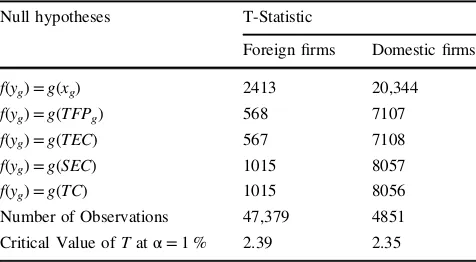
compar-ing of kernel distribution of output growth and input growth through testing the null hypothesis H0:f(yg)=g(xg), we could analyze whether output growth distribution can be explained by input growth. When theH0is rejected, then it

could be concluded that total factor productivity variations signiﬁcantly explain the variations of the output growth distribution. In addition, to evaluate the contribution of input growth on the variation of output growth, we test the null hypothesisH0:f(yg)=g(TFPg). When theH0is rejected,

then it could be concluded that input growth can be sig-niﬁcantly sources of the changes in output growth dis-tribution. As mention before, TFP growth is decomposed into three components of productivity. To assess which the most important component in explaining the variations in the TFP growth distribution, we consider three hypotheses, such asH0:f(yg)=g(TC),H0:f(yg)=g(TEC) andH0:f(yg) =_g₍_SEC_{). When we reject the} _H₀_{, then the component of}

productivity has a signiﬁcant role in explaining the TFP growth.

5 Empirical results

5.1 The FDI spillover effects on the_ﬁrms_’productivity performances

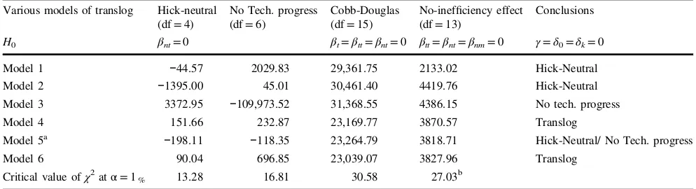
Based on the methodology that has been discussed in Sect. 3, we can construct six alternative models of the stochastic production frontier with inefﬁciency effects.15The accuracy of FDI spillover estimates requires an appropriate functional form of stochastic production frontier. To ﬁnd an appro-priate functional form that represents the data, various sub-models of the translog are tested against a translog model using generalized likelihood ratio (LR) statistic test. The results of null hypotheses tests of various sub-models of the translog against translog model are reported in Table4.

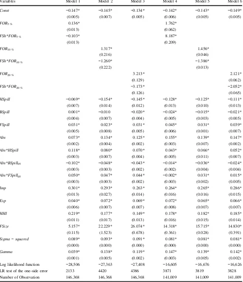
The estimated results of the stochastic production frontier with inefficiency effects in Eq. (10a) and (b) could be divided into three parts; the estimated coefficients of inputs on the production function, the estimated coefficients of

FDI spillover on production function and inefﬁciency

function. Moreover, the particular interest of this study is on the estimated FDI coefficients of the production function and inefficiency function. Hence, we analyze initialy the FDI spillover effects on the firms’ productivity and effi -ciency, then we analyze the coefficients of the production function through evaluating the output elasticity with respect to each input as well as elasticity of substitution between capital and labour. The results of FDI spillover

15

(15)

effects on thefirms’productivity are reported in Table5and on thefirms’efficiency are presented in Table6. And, the results of the estimated coefficients of inputs on production functions are provided in Appendix Table12.

We start by focusing on all the dummiesFOR in

pro-duction functions (in Table 5). They carry rather large, statistically significant coeffcients, suggesting that foreign establishments have comparable high levels of productivity. However, the coefficients of the dummy FORin the inef-ficiency functions (in Table6) are positive and statistically significant. Those positive signs indicates that foreignfirms are less efficient than domestic firms, keeping other vari-ables constant.

By evaluating the interacting foreign share with the dummyFORin production functions, the degree of foreign ownership in establishments seem to have negative and significant effect on productivity, except for Model 1 and 4. These results show that increases the degree of foreign ownership negatively affectfirms’ productivity. This nega-tive spillover, such as market stealing effect causes foreign firms forcing local firms to cut their production. On the other hand, the estimated interacting dummy variables with foreign equity in the inefficiency functions have negative signs and statistically significant, except for Model 4. This describes that increasing share of foreign equity associated with reducing inefficiency.

More important for the purpose of this study, the pre-sence of intra-industry and inter-industry spillovers are addressed. The positive and signiﬁcant coefﬁcient on the

HSpillin Table5suggests thatfirm’s output increases when the share of output of foreignfirm within the same market rises. This study finds evidence of horizontal spillovers from foreign firms to domestic firms, which is consistent with our previous empirical studies on the Indonesian manufacturing sector which use a conventional approach of

production function (Blalock and Gertler 2008; Sjöholm

1999). The negative signs of HSpill and statistically dif-ferent from zero appear in all models in Table 6. These indicate that the competitive effects of foreign firms do reduce the inefficiency of domesticfirms through the same market. Indigenous establishments may be able to reduce innovation costs by observing and imitating the foreign invested companies.

To examine vertical spillovers on thefirms’productivity perfornmance, we deliberate on all the models in Table5as well as Table6. The coefficients ofBSpillandFSpillin all models in Tables 5 and 6 have the similiar signs and sig-nificancies, except a BSpill coefficient in Model 1 in Table 6.16 The negative and statistically significantBSpill

coefficients seem to appear in all models of production functions (see Table5). The negative productivity spillovers in the upstream markets may appear if the intermediate inputs produced by local suppliers are not used intensively by foreign affiliates. They may import their intermediate inputs. Therefore, the negative backward productivity spil-lovers arise in the upstream markets. In addition, the negative backward spillovers could arise when foreign companies have greater bargaining power than local com-panies. This condition may lead to unfavouring contractual agreements towards local enterprises and may squeeze their profit. Hence, the productivity of local suppliers will decrease. But, the coefficients of BSpill in inefficiency functions, except a coefficient in Model 1 (see Table 6a) have negative signs and statistically diffrent from zero.

These may indicate that the presence of foreign ﬁrms

Table 4 Hypotheses testing of various models of translog

Various models of translog Hick-neutral (df=₄₎

Model 1 −44.57 2029.83 29,361.75 2133.02 Hick-Neutral

Model 2 −1395.00 45.01 30,461.40 4419.76 Hick-Neutral

Model 3 3372.95 −109,973.52 31,368.55 4386.15 No tech. progress

Model 4 151.66 232.87 23,169.77 3870.57 Translog

Model 5a −198.11 −118.35 23,264.79 3818.71 Hick-Neutral/ No Tech. progress

Model 6 90.04 696.85 23,039.07 3827.96 Translog

Critical value ofχ2atα=₁_% _13.28 _16.81 _30.58 _27.03b

a

For Model 5, we further conduct testing for hick-neutral against no-technological progress. (Since the LR statistic test (=_{79.76) is greater than the} critical value ofχ2atα=_{1 % (}=_{9.21), we conclude that hick-neutral is used for estimating Model 5.)}

b_{Using critical values of Mix}_χ2_at_α₌_{1 %. (This critical value is taken from Table}₁_{of Kodde and Palm (}₁₉₈₆₎₎

16

As mention in footnote 3, this study consider using I–O table of year 2000 instead of year 2005 for calculating inter-industry linkages for year of 2003 and year of 2004 and the estimated coefﬁcients of

(16)

generate positive spillovers onﬁrm’s technical efﬁciency in the upstream industries.

On the other hand, the coefficients ofFSpill in produc-tion and inefficiency functions are positive and statistically different from zero (see Table 5a and b). These finding indicate that the linkages of foreign firms to downstream industries provide technological gains to domestic buyers. Sales of these inputs by MNCs may be accompanied by provision of complementary services that may not be

available in connection with imports. Foreign ﬁrms have incentives to improve domesticﬁrm’s productivity through input cost reduction and quality improvement in return,

which then lead to productivity beneﬁts. However, the

positive sign in inefficiency functions indicate that the presences of foreign firms generate negative spillovers on firm’s technical efficiency in the downstream industries.

Even though the inter-industry spillovers do not entirely enhance ﬁrms’ productivity performance, the presence of Table 5 The estimated coefﬁcients on production functions

Variables Model 1 Model 2 Model 3 Model 4 Model 5 Model 6

FOR5 % 0.068* 1.711*

(0.011) (0.061)

FSh*FOR5 % 0.017 8.242*

(0.012) (0.209)

FOR10 % 1.247* 1.388*

(0.216) (0.011)

FSh*FOR10 % −1.142* −1.282*

(0.219) (0.009)

FOR20 % 3.137* 2.041*

(0.130) (0.060)

FSh*FOR20 % −3.044* −1.937*

(0.127) (0.062)

HSpill 0.072* 0.062* 0.062* 0.051* 0.063* 0.065*

(0.006) (0.008) (0.007) (0.007) (0.006) (0.007)

BSpill −0.011* −0.024* −0.026* −0.022* −0.021* −0.022*

(0.002) (0.004) (0.003) (0.003) (0.003) (0.003)

FSpill 0.037* 0.043* 0.044* 0.039* 0.038* 0.039*

(0.002 (0.004) (0.003) (0.003) (0.003) (0.003)

Abs 0.255* 0.282* 0.281* 0.274* 0.268* 0.270*

(0.002) (0.002) (0.002) (0.002) (0.002) (0.002)

Abs*HSpill 0.025* −0.003 −0.013*** −0.009 −0.006* −0.008

(0.006) (0.009) (0.007) (0.006) (0.002) (0.006)

Abs*BSpill −0.077* −0.038* −0.039* −0.023* −0.030* −0.026*

(0.003) (0.003) (0.003) (0.002) (0.001) (0.003)

Abs*FSpill 0.056* 0.040* 0.043* 0.020* 0.030* 0.025*

(0.003) (0.004) (0.003) (0.003) (0.002) (0.003)

Imp 0.044* 0.059* 0.044* 0.063* 0.057* 0.072*

(0.011) (0.020) (0.011) (0.012) (0.011) (0.011)

Exp 0.004 0.023* 0.023* 0.026* 0.021* 0.021*

(0.004) (0.004) (0.004) (0.004) (0.004) (0.004)

HHI 0.119* 0.074* 0.062* 0.080* 0.076* 0.079*

(0.009) (0.011) (0.009) (0.010) (0.010) (0.009)

FSize 5.337* 22.441* 26.295* 14.488* 15.884* 14.997*

(0.118) (1.525) (0.679) (0.362) (0.036) (0.392)

Number of Observations 146,368 146,368 146,368 141,009 141,009 141,009

Standard errors are in parentheses. The estimated coefﬁcients in Model 1 to Model 3 are using material input criteria 1 and in Model 4 to Model 6 are using material input criteria 2

(17)

Table 6 The estimated coefﬁcients on inefﬁciency functions

Variables Model 1 Model 2 Model 3 Model 4 Model 5 Model 6

Const −0.147* −0.145* −0.134* −0.142* −0.143* −0.149*

(0.005) (0.007) (0.005) (0.006) (0.005) (0.005)

FOR5 % 0.136* 1.762*

(0.013) (0.062)

FSh*FOR5 % −0.103* 8.187*

(0.013) (0.209)

FOR10 % 1.317* 1.456*

(0.216) (0.046)

FSh*FOR10 % −1.260* −1.386*

(0.222) (0.013)

FOR20 % 3.213* 2.121*

(0.129) (0.062)

FSh*FOR20 % −3.173* −2.052*

(0.126) (0.065)

HSpill −0.069* −0.154* −0.145* −0.128* −0.125* −0.111*

(0.007) (0.014) (0.012) (0.013) (0.010) (0.013)

BSpill 0.001* −0.010 −0.020* −0.024* −0.015* −0.021*

(0.004) (0.007) (0.004) (0.005) (0.003) (0.005)

FSpill 0.031* 0.023* 0.031* 0.045* 0.031* 0.039*

(0.005) (0.008) (0.005) (0.006) (0.001) (0.007)

Abs 0.073* 0.134* 0.125* 0.155* 0.139* 0.147*

(0.002) (0.004) (0.002) (0.003) (0.007) (0.002)

Abs*HSpill 0.118* 0.080* 0.070* 0.043* 0.066* 0.052*

(0.003) (0.007) (0.004) (0.005) (0.011) (0.007)

Abs*BSpill05 −0.102* −0.048* −0.043* −0.014* −0.036* −0.024*

(0.003) (0.003) (0.002) (0.002) (0.004) (0.004)

Abs*FSpill05 0.050* 0.047* 0.044* −0.002* 0.031* 0.015*

(0.003) (0.003) (0.002) (0.003) (0.002) (0.005)

Imp 0.301* 0.293* 0.263* 0.264* 0.265* 0.286*

(0.013) (0.027) (0.014) (0.016) (0.016) (0.015)

Exp 0.040* 0.072* 0.069* 0.072* 0.065* 0.066*

(0.006) (0.007) (0.007) (0.008) (0.007) (0.007)

HHI 0.219* 0.177* 0.149* 0.178* 0.182* 0.185*

(0.011) (0.017) (0.013) (0.016) (0.015) (0.014)

FSize 5.157* 22.229* 26.074* 14.318* 15.715* 14.830*

(0.115) (1.523) (0.678) (0.361) (0.028) (0.391)

Sigma−squared 0.089* 0.093* 0.091* 0.081* 0.081* 0.081*

(0.000) (0.000) (0.000) (0.000) (0.000) (0.000)

Gamma 0.039* 0.138* 0.119* 0.147* 0.139* 0.142*

(0.001) (0.005) (0.002) (0.003) (0.005) (0.002)

Log likelihood function −28,506 −27,363 −27,408 −16,605 −16,676 −16,626

LR test of the one-side error 2133 4420 4386 3871 3819 3828

Number of Observation 146,368 146,368 146,368 141,009 141,009 141,009

Standard errors are in parentheses. The estimated coefﬁcients in Model 1 to Model 3 are using material input criteria 1 and in Model 4 to Model 6 are using material input criteria 2