POSE VERSUS STATE: ARE SENSOR POSITION AND ATTITUDE SUFFICIENT FOR
MODERN PHOTOGRAMMETRY AND REMOTE SENSING?
I.Colomina1, M.Bl´azquez2
1Centre Tecnol`ogic de Telecomunicacions de Catalunya
Av. Carl Friedrich Gauss 7, Parc Mediterrani de la Tecnologia, Castelldefels, Spain, [email protected] 2GeoNumerics, Josep Pla 82, Barcelona, Spain, [email protected]
KEY WORDS:sensor state, sensor orientation, sensor calibration, spatio-temporal sensor calibration, image deblurring, focal-plane shutter camera models.
ABSTRACT:
We investigate the advantages of using what we callsensor state parametersorsensor stateto describe the geometrical relationship between a sensor and the 3D space or the 4D time-space that extend the traditional image pose or orientation (position and attitude) to the image state. In our concept, at some point in timet, the sensor state is a 12-dimensional vector composed of four 3-dimensional subvectorsp(t),v(t),γ(t)andω(t). Roughly speaking,p(t)is the sensor’s position,v(t)its linear velocity,γ(t)its attitude andω(t) its angular velocity. It is clear that thestateconcept extends theposeororientationones and attempts to describe both a sensor’s statics (p(t),γ(t)) and dynamics (v(t),ω(t)). It is also clear that ifp(t),γ(t)are known for alltwithin some time interval of interest, then
v(t)andω(t)can be derived from the former.
We present three methods to compute the state parameters, two for the continuous case and one for the discrete case. The first two methods rely on the availability of inertial measurements and their derived time-Position-Velocity-Attitude (tPVA) trajectories. The first method extends the INS mechanization equations and the second method derives the IMU angular velocities from INS mechanization equations’ output data. The third method derives lineal and angular velocities from relative orientation parameters.
We illustrate how sensor states can be applied to solve practical problems. For this purpose we have selected three cases: multi-sensor synchronization calibration, correction of image motion blur (translational and rotational) and accurate orientation of images acquired with focal-plane shutters.
1 INTRODUCTION AND MOTIVATION
For many years, sensor position and attitude parameters —orient-ation parameters— have served well the needs of photogram-metry, remote sensing and their sister and customer disciplines; i.e., the traditional 3D reconstruction tasks with traditional sen-sors can be performed with them. However, in recent times, the complexity and variety of photogrammetric and remote sensing tasks as well as the variety of sensing devices has blossomed. The cost of the sensing devices in use —including but not lim-ited to cameras— ranges from a few hundred to a million euros ( C). Sensing techniques have diversified from film cameras to digital ones (including multispectral and hyperspectral frequency bands), to LiDAR and radar. In addition to geometric 3D scene reconstruction (a genuine photogrammetric task) and to terrain classification (a genuine remote sensing tasks), images are re-stored, integrated with other images, geometrically and radio-metrically calibrated, time aligned to a common time reference frame, and processed in many other ways. For this purpose, it is many times convenient to know the sensor’s velocity or the ratio of change of its attitude matrix.
In this paper we explore the convenience, advantages and dis-advantages of using what we call “sensor state parameters” — “camera state parameters” when appropriate— to describe the ge-ometrical relationship between a sensor and the 3D space or the 4D time-space. In our concept, at some point in timet, the sensor state is a 12-dimensional vector composed of four 3-dimensional subvectorsp(t),v(t),γ(t)andω(t). Roughly speaking,p(t)is the sensor’s position,v(t)its linear velocity,γ(t)its attitude and
ω(t)its angular velocity. It is clear that the “state” concept ex-tends the “pose” or “orientation” ones and attempts to describe both a sensor’s statics (p(t),γ(t)) and dynamics (v(t),ω(t)). It is also clear that ifp(t),γ(t)are known for alltwithin some time
interval of interest, thenv(t)andω(t)can be derived from the former. However, this is not always the case, as it is inconvenient to keep the camera trajectory{p(t), γ(t)}tand make it available to potential users.
First, we propose a modification of the INS mechanization equa-tions to include the angular velocity as an unknown state. Sec-ond, we describe a post-processing method where measured an-gular rates are corrected with the anan-gular rate sensors estimated systematic errors. Last, we derive sensor linear and angular ve-locities from relative orientation parameters.
Three theoretical cases will be presented: multi-sensor synchro-nization calibration, correction of image motion blur (transla-tional and rota(transla-tional) and accurate orientation of images acquired with focal-plane shutters.
In the multi-sensor synchronization calibration, i.e., in the esti-mation of time delays between the instrumental time coordinate reference frames (CRFs) of the various sensors of a system, we will build upon our own results where we used the knowledge of
p(t),v(t),γ(t)andω(t)for the estimation of theδtj
ibetween the
CRFs of instrumentsiandj. We claim, that using the 12 state parameters makes the use of the aerial control models in our ex-tended aerial control models straightforward and, therefore, the knowledge of the state parameters and their covariance matrices becomes a big advantage.
In image translational and rotational motion deblurring, we build upon the technique presented by N. Joshi in 2010. N. Joshi used, for the first time, inertial measurement units for dense, per-pixel spatially-varying image deblurring. In our proposal their method can be further simplified because we propose to use INS/GNSS integrated results and not only INS results, thus avoiding their smart, though complex, INS drift correction.
In the orientation of images acquired with cameras whose shutter is of the focal-plane type, we propose a new orientation model that extends the classical colinearity equations and that takes into account that, although all image rows are exposed during a time interval of the same length, not all rows are exposed with the same central time. For this purpose, the twelve image state parameters are used to derive more accurate orientation parameters for each image row.
The core of the paper is organized in four sections, 2 to 5: in-troduction of the sensor state parameters (section 2; with frame, notation and naming conventions in section 2.1 and with the def-inition of sensor states in 2.2); mathematical structure of pose and state parameters (section 3); their computation (section 4); and some of their applications (section 5; to image deblurring in section 5.1, to multi-sensor system synchronization in section 5.2 and to orientation and calibration of low-cost and amateur cam-eras in section 5.3).
2 SENSOR STATE PARAMETERS
2.1 Reference frames, notation and naming conventions
We begin by describing the coordinate systems and reference frames —i.e.,coordinate reference frames(CRF) or justframes— of our models.
For the object frame we have selected the local [terrestrial] geode-tic cartesian frame parameterized by the east (e), north (n) and up (u) coordinates. This type of frame will be denoted byl. cwill be camera or imaging instrument frame andbthe inertial mea-surement unit (IMU) frame. When mounted on a vehicle, we will assume that bothcandbare defined following the (forward-left-up) convention.
In the equations we will use superscripts to indicate the frame of vectors like inpl
orvl
; superscripts and subscripts to indicate the “to” and “from” frames, respectively, of rotation matrices and their angular parametrization like inR(γ)l
c or γlc; superscripts
and double subscripts like inΩ(ω)c
lcorγclcto indicate the angular
velocity matrix or vector of the framecwith respect to the frame
lmeasured in the framec. Time dependency, also for frames, will be written as usually like inpl(t),γc
lc(t)orxc(t).
As usual, the superscriptTwill indicate transpose of a vector or matrix. If clear from the context, in order to simplify notation and facilitate lecture, we will avoid its use and write(e, n, u)instead of the formally correct(e, n, u)T
.
Last, if a rotation or angular velocity matrix is parametrized by anglesγl
2.2 The concept of sensor state
We definesl
c the state of a sensing instrumentor, simply, the
sensor stateorsensor state parametersas the duodecuple —the quadruple of triples—
the instrumental CRF in thel frame andvl its velocity vector. γl
cis a parametrization ofR(γ)lc, the rotation matrix fromctol
—the sensor attitude matrix— andωc
lcis the vector of
instanta-neous angular velocities of thecframe with respect to thelframe,
referred to thecframe. ωc
lccan be also seen as a
parameteriza-tion of the angular velocity skew-symmetric matrixΩ(ω)c lc—the
We will writeW(n)to denote the set of all real skew-symmetric
n×nmatrices. Following the notation conventions of section 2.1 in the sequel we will writeR(γ)l
c andΩ(ω)clc for the rotation
and angular velocity matrices respectively. Last, when it is clear from the context we will write the sensor state defined in 1 as (p, v, γ, ω),(p, v, R(γ),Ω(ω))or, simply,(p, v, R,Ω).
Clearly, the sensor state parameters(p, v, γ, ω)generalize and in-clude the sensor pose or exterior orientation parameters(p, γ). If they are time dependent differentiable functions they are related as follows
We borrowed the term “state” from mechanics and navigation.
3 MATHEMATICAL STRUCTURE OF POSE AND STATE PARAMETERS
The sensor’s pose or exterior orientation parameterspl
andγl
c—
strictly speakingpl
candγcl— describe the translation and rotation
of the sensing instrument 3D reference framecwith respect to a world or object 3D reference framel. In other words,(pl, γl
c)
represent a rigid body transformation inℜ3fromxcinxl
xl=R(γ)lcx c
+pl. (3)
In the mathematical abstraction, the set of affine mapsϕofℜ3,
ϕ(x) =Rx+p, whereR∈SO(3)andp∈ ℜ3with the binary operator·defined as
(ϕ2·ϕ1)(x) =ϕ2(ϕ1(x))
is the group of rigid motionsSE(3), theSpecial Euclideangroup ofℜ3. We recall thatSO(3)is theSpecial Orthogonalgroup of
ℜ3—i.e., the group of rotation matrices inℜ3— and thatSE(3) is a semidirect product ofSO(3)andℜ3,SE(3) =SO(3)⋊ℜ3
(Gallier, 2011).
Let us now assume that the sensor moves; i.e., that the reference framecis a function of timec(t)and that the reference framel
remains static. Then, it holds
does not move with respect to thec(t)instrumental reference frame; i.e.,x˙c(t)= 0. In this case
of a pointxc(t), static with respect to the instrumental reference framec(t), can be derived fromp(t),v(t),γ(t)andω(t). There-fore,p(t),v(t),γ(t)andω(t)characterize the dynamics of the instrument.
4 COMPUTATION OF SENSOR STATES
In this section we present two approaches to estimate the sensor state parameters; one based on the measurements and/or results of INS/GNSS integration and one based on the relative orienta-tion and angular velocities between consecutive images of image sequences.
4.1 States from inertial and GNSS measurements
Sensors states can be computed in a number of ways. Since the beginning of the nineteen nineties integrated INS/GNSS systems (Schwarz et al., 1993) have been used to directly estimate or to in-directly contribute to the estimation of the orientation parameters of imaging instruments. In the latter case the estimation method is known as Integrated Sensor Orientation (ISO) and in the for-mer as Direct Georeferencing (DG) or Direct Sensor Orientation (DiSO). When neither INS/GNSS nor GNSS aerial control ob-servations are available (or of sufficient precision and accuracy) sensor orientation has to resort to the old Aerial Triangulation (AT) or Indirect Sensor Orientation (InSO).
INS/GNSS systems provide high-frequency —typically, from 50 to 1000 Hz— time-Position-Velocity (tPVA) trajectory solutions that, as indicated, have been used for DiSO or ISO orientation in P&RS. As already pointed in (Bl´azquez, 2008), the velocity information of INS/GNSS-derived trajectories has not been fully exploited. The tPVA trajectories can be easily transformed into imaging instruments orientation parameters and velocity param-eters by propagating them through lever arms (spatial shifts) and rotation matrices (angular shifts, also known as boresight angles) into a part of the state parameterssl
c, namely the nine components
(pl, vl, γl
c). However, for the purposes of this article, the imaging
instrument angular velocitiesωc
lcare still missing.
The tPVA INS/GNSS-derived trajectories result from the [numer-ical] integration of the inertial [stochastic differential] equations of motion also known as inertial mechanization equations (Jekeli, 2001, Titterton and Weston, 2004). These stochastic differential equations (SDE) generate the corresponding stochastic dynami-cal system (SDS) that, together with external static [update] mea-surements can be processed with a Kalman filtering and smooth-ing strategy. GNSS carrier phase measurements or their derived positions are the usual update measurements. In other words, INS/GNSS integration as usual with an augmented state vector with the inertial measurement unit (IMU) error states and, possi-bly, other error modeling states. If we take into account that
Ω(ω)clc=R
wherebis the coordinate reference frame (CRF) of the inertial measurement unit, our problem would be solved if we were able to estimateωb
lbin or from the Kalman filter and smoother.
In order to do so, we can use the IMU angular rate raw measure-ments and correct them according to the IMU angular rate cali-bration model and states. Or we can introduce a new [3D vector] state in the KFS forωb
lb. There are advantages and
disadvan-tages to each approach. In the latter approach, the extension of the KFS state vector withωb
lbrequires a dynamical model forωlbb
be it through the trivial random walk modelω˙b
lb= 0 +wwith
a large variance forwand then use the IMU angular rate mea-surements as update meamea-surements. This would introduce update steps at the frequency of the IMU measurements which is com-putationally expensive and not recommended for the numerical integration algorithms. However the solution trajectory is con-ceptually “clean” and the state covariance matrices are directly
available from the trajectory solution. The former approach, al-though less rigorous in principle, requires no modification of the INS/GNSS software which, for the P&RS community is more at-tractive and, in general, has less impact in the existing installed software base and production lines.
4.2 States from orientation parameters
In the previous section we have described how to determine the sensor state parameters from INS/GNSS systems. In general we favor this approach: INS/GNSS integration delivers an [almost] drift-free and [sufficient] high frequency trajectory from where sensor states can be interpolated. Of course, “almost” and “suf-ficient” are context dependent attributes. However, there may be situations where dense trajectory information is not available and, still, where sensor state parameters are required. In the case of image sequences like video images or photogrammetric blocks, a sensor’s state parameters can easily be derived from its own and neighboring exterior orientation parameters if the latter are time tagged. Let us assume then the sequence{ol
c(ti)}i of exterior
instance, computing the relative attitude matrixRk k−1
and noting that the matrix logarithm of a rotation matrix is a skew symmetric matrix (Higham, 2008)
which defines a recursive relation that can be exploited in the con-text of an extended bundle adjustment from starting and ending non-rotating instruments.
5 SOME APPLICATIONS
5.1 Image deblurring
Motion blurring occurs when, during the time exposure of an im-age, either the image moves, or imaged objects move or both. Motion blur becomes apparent for combinations of relatively long exposure times and/or rapid motions. The problem is well known in photogrammetry and traditionally solved with [mechanical] forward motion compensation (FMC) techniques under the as-sumption of dominant translational and negligible rotational mo-tion effects. FMC systems add complexity —therefore cost— to the image acquisition systems and, sometimes, like in UAS photogrammetry, they also add non carriable critical additional weight. (The topic of motion blur in UAS photogrammetry has been recently addressed in (Sieberth et al., 2013).) Image deblur-ring is an area of growing interest.
An observed blurred imageBcan be thought as an ideal, original, unblurred imageL—thelatentimage— that has been degraded by motion. It is customary to model this image degradation as
B+v=L⊗k (8)
wherevis positive additive noise andkis a convolution kernel that translates the camera/object 3D motion into 2D image “mo-tion” that, in imaging terms, can be interpreted as a point spread function (PSF).kis also known as theblur function. Image de-blurring is the process of recoveringLfrom knownB, knownv
and, known or unknown,k. Image deblurring is a deconvolution problem. If the blur functionkis known,Lcan be recovered with a non-blind deconvolution method. However, for images with just orientation parameters(pl(t), γl
c(t)),kis unknown and
must be recovered together withL with a blind-deconvolution method. Blind deconvolution is an ill-posed problem, as the ob-served blurred imageB contributes insufficient measurements. If the camera trajectory{pl(t), vl(t), γl
c(t), ω c
lc(t)}tand the
im-aged object are known,kcan be unambiguously determined. Ac-cording to this, in P&RS, depending on the phase of the map production line,kcan be determined. Moreover, considering the short exposure times and long distances camera-object,kcan be approximated with just the knowledge of the image state param-eters at the central exposure timet, pl(t), vl(t), γl
c(t), ωclc(t)
, or of the state parameters and the average height above ground.
For knownk, the Lucy-Richardson iterative deconvolution me-thod, also known as the Richardson-Lucy algorithm (Lucy, 1974), is usually applied. An example of a blind deconvolution algo-rithm, for unknown or poorly determinedkcan be found in (Lam and Goodman, 2000). Blind deconvolution is more complex and inefficient that non-blind deconvolution and therefore, consider-able research has been devoted to estimate or measure, in one way or another, camera/image motion parameters. In (Lel´egard et al., 2012) a method without the knowledge of the motion pa-rameters is presented although the use of inertial measurements is suggested as an alternative. In (Shah and Schickler, 2012) rota-tional motion is extracted from single images by means of trans-parency cues of blurred objects in the image. In (Joshi et al., 2010) translation and rotational motion is derived from inertial measurements and, from those, an aided blind deconvolution al-gorithm is proposed.
Since exposure times in aerial photography are short, the use of the image state parameters shall be sufficient to characterize the dynamics of the image during the exposure time interval.
The (Joshi et al., 2010) approach can be simplified if, instead of a free INS trajectory solution, a driftless INS/GNSS or any other driftless trajectory is used; i.e., the blur function kernelk can easily be computed.
5.2 Sensor space-time calibration
In (Bl´azquez, 2008) and (Bl´azquez and Colomina, 2012) we pre-sented a concept and the corresponding mathematical models for four dimensional space-time calibration of multi-sensor P&RS data acquisition systems as an extension of the integrated sensor orientation method. The key idea behind the concept was that INS/GNSS-derived linear and angular velocity parameters can be used to link synchronization errors to spatial errors. In this way, spatial control information —aerial or terrestrial— and an appropriate block geometry allow for simultaneous sensor cali-bration, synchronization error correction (time calibration) and even GNSS-related shift parameter estimation. The mathemati-cal models are not reproduced here and the reader is referred to the mentioned references for details.
5.3 Orientation of low-cost and amateur cameras
It is often the case, that mass-market small-format cameras are used for mapping professional applications not only because of
❄r
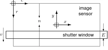
Figure 1: Focal-plane shutter parameters.
their low cost but also because of their low weight, relative high resolution —currently, up to 25 Mpx,— excellent optics and, in general, high performance-to-price ratio. The exposure timeeof many, if not most, of these cameras is controlled by a focal-plane shutter located in front of the image sensor near the camera focal plane. Focal-plane shutters move a window aperture to uncover the image sensor in such a way that every pixel is exposed to light during a time interval of lengthe. Thus, iftis the image central exposure time, not all pixels or row of pixels (line) are exposed during the time interval[t−e/2, t+e/2]. Instead, the actual exposure time intervalT(l)of a linelis
T(l) = [t+ ∆t(l)−e/2, t+ ∆t(l) +e/2]
wheree=E/v,∆t(l) = (l−n/2)/v,Eis the width (height) of the shutter sliding window,nis the row size (height) of the image sensor andvis the moving speed of the window. We will say that the central exposure time of linelor, simply, the exposure time
t(l)of linelist(l) =t+ ∆t(l). Figure 1 depicts a simplified focal-plane shutter concept and relates it to the parametersE,n
andv. For instance, for a a Sony NEX-7 camera with exposure time intervals of 1/4000 s,v≈35m/s.
In the above formulas we have used a(row,column)coordinate system whose origin is in the (up, left) image corner, where rows (lines) and columns are numbered0,1, . . .top-to-down and left-to-right respectively, and where the shutter window moves top-to-down. We used the traditional photogrammetric(x, y) PPS-centered coordinate system, then
T(y) = [t+ ∆t(y)−e/2, t+ ∆t(y) +e/2]
where∆t(y) =−y/v, and wheree,E,n,vhave to be given in the appropriate physical units. Analogously, we will say that the central exposure time, or exposure time,t(y)of lineyist(y) =
t+ ∆t(y).
For the sake of clarity we will now neglect image distortions and atmospheric refraction. If the image state is pl, vl, γl
c, ωllc
and a ground pointxlis projected into the image point(x, y), then
we can write the classical colinearity condition
xl=pl(x, y) +µ·Rl
The above equations 9 and 10 are rigorous models for focal-plane shutter cameras that take into account the non-simultaneous imaging effect of their shutter mechanism. Similar to the geome-try of pushbroom cameras, if pl, vl, γc, ωl l
lc
are known, image-to-ground —in general, image-to-object— transformations are straightforward. On the contrary, object-to-image transforma-tions may involve iterative —simple and fast, though— algo-rithms.
6 CONCLUSIONS
We have explored the extension of camera exterior orientation or pose parameters (position and attitude) to what we call camera or imagestate parameters(position, velocity, attitude and attitude rates). The state parameters capture the dynamics of the camera.
We have shown the advantages of the state parameters over the orientation parameters with three examples: image deblurring, spatio-temporal calibration of imaging instruments and orienta-tion of low-cost amateur cameras with focal-plane shutters. In the three cases, the state parameters, as we have formulated them, ap-pear in a natural and independent way when trying to cope with some problems caused and/or related to the sensing instrument motion.
We plan to further investigate the mathematical structure of the state parameters in theℜ3× ℜ3×SO(3)×W(3)space and the estimation of angular velocity states in the INS/GNSS Kalman filter and smoother. We also plan to experimentally asses the practical usefulness of the proposed methods for image deblur-ring and orientation of focal-plane shutter camera images.
7 ACKNOWLEDGEMENTS
The focal plane shutter velocityv(section 5.3) was measured by E. Fern´andez and E. Angelats (CTTC).
The research reported in this paper has been partially funded by the GSA project GAL (Ref. FP7-GALILEO-2011-GSA-1, FP7 Programme, European Union).
The project DINA (Ref. SPTQ1201X005688XV0, Subprogama Torres y Quevedo, Spain) has also partially funded this research.
REFERENCES
Bl´azquez, M., 2008. A new approach to spatio-temporal cali-bration of multi-sensor systems. ISPRS - International Archives of the Photogrammetry, Remote Sensing and Spatial Information Sciences XXXVII-B1, pp. 481–486.
Bl´azquez, M. and Colomina, I., 2012. On INS/GNSS-based time synchronization in photogrammetric and remote sensing multi-sensor systems. PFG Photogrammetrie, Fernerkundung und Geoinformation 2012(2), pp. 91–104.
Gallier, J., 2011. Geometric methods and applications for com-puter science and engineering. Springer, New York, NY, USA.
Higham, N., 2008. Functions of Matrices: Theory and Computa-tion. Society for Industrial and Applied Mathematics, Philadel-phia, PA, USA.
Jekeli, C., 2001. Inertial navigation systems with geodetic appli-cations. Walter de Gruyter, Berlin, New York.
Joshi, N., Kang, S., Zitnick, C. and Szeliski, R., 2010. Image deblurring using inertial measurement sensors. In: ACM SIG-GRAPH 2010 papers, SIGSIG-GRAPH’10, ACM, New York, NY, USA, pp. 30:1–30:9.
Lam, E. Y. and Goodman, J. W., 2000. Iterative statistical ap-proach to blind image deconvolution. J. Opt. Soc. Am. A 17(7), pp. 1177–1184.
Lel´egard, L., Delaygue, E., Br´edif, M. and Vallet, B., 2012. Detecting and correcting motion blur from images shot with channel-dependent exposure time. ISPRS - Annals of the Pho-togrammetry, Remote Sensing and Spatial Information Sciences I-3, pp. 341–346.
Lucy, L., 1974. An iterative technique for the rectification of observed distributions. Astronomical Journal 79(6), pp. 745–754.
Schwarz, K., Chapman, M., Cannon, M. and Gong, P., 1993. An integrated INS/GPS approach to the georeferencing of remotely sensed data. Photogrammetric Engineering and Remote Sensing 59(11), pp. 1167–1674.
Shah, C. and Schickler, W., 2012. Automated blur detection and removal in airborne imaging systems using IMU data. ISPRS -International Archives of the Photogrammetry, Remote Sensing and Spatial Information Sciences XXXIX-B1, pp. 321–323.
Sieberth, T., Wackrow, R. and Chandler, J., 2013. Automatic isolation of blurred images from UAV image sequences. ISPRS - International Archives of the Photogrammetry, Remote Sensing and Spatial Information Sciences XL-1/W2, pp. 361–366.
Titterton, D. and Weston, J., 2004. Strapdown inertial navigation technology, (2nd edition). Progress in Astronautics and Aeronau-tics, Vol. 207, American Institute of Aeronautics and Astronau-tics, Reston, VA, USA.