Full Terms & Conditions of access and use can be found at
http://www.tandfonline.com/action/journalInformation?journalCode=ubes20
Download by: [Universitas Maritim Raja Ali Haji], [UNIVERSITAS MARITIM RAJA ALI HAJI
TANJUNGPINANG, KEPULAUAN RIAU] Date: 11 January 2016, At: 20:21
Journal of Business & Economic Statistics
ISSN: 0735-0015 (Print) 1537-2707 (Online) Journal homepage: http://www.tandfonline.com/loi/ubes20
Comment
Barbara Rossi
To cite this article: Barbara Rossi (2014) Comment, Journal of Business & Economic Statistics, 32:4, 510-514, DOI: 10.1080/07350015.2014.956875
To link to this article: http://dx.doi.org/10.1080/07350015.2014.956875
Published online: 28 Oct 2014.
Submit your article to this journal
Article views: 85
View related articles
Comment
Barbara R
OSSIDepartment of Economics, ICREA-Universitat Pompeu Fabra, GSE, and CREI, Barcelona, Spain ([email protected])
1. INTRODUCTION
Several articles have attempted to evaluate the performance of central banks’ forecasts. Among them, for example, Romer and Romer (2000), Faust and Wright (2009), Edge and G¨urkaynak (2010), Christoffel, Coenen, and Warne (2010), Edge, G¨urkay-nak, and Kisacikoglu (2013), Edge, Kiley, and Laforte (2010), and G¨urkaynak, Kisacikoglu, and Rossi (2013) evaluated the forecasting performance of Greenbook forecasts and/or macroe-conomic models typically used in Central Banks. However, none of these articles focuses on evaluating forecasts during the recent financial crisis, which is instead the goal of Alessi et al. (2014). Alessi et al. (2014) document the macroeconomic forecasting experience of the European Central Bank (ECB) and the Federal Reserve Bank of New York (FRBNY) during the recent financial crisis of 2007–2008. Such analysis is extremely important since the forecasts of key macroeconomic variables made at those in-stitutions were the inputs of the extraordinary monetary policy measures taken by the central banks at the time of the crisis. The authors provided a careful description of the institutional background and forecasting process at both central banks, par-ticularly focusing on evaluating point and density forecasts. Re-garding point forecasts, the authors found that the mean squared forecast errors (MSFEs) of real GDP growth of the two insti-tutions were comparable, and that they increased substantially during the financial crisis (between five and six times) relative to the precrisis period in both institutions. The point forecasts of inflation at the FRBNY were comparable before and after the crisis, whereas those of the ECB worsened substantially. Alessi et al. (2014) note that early signals from financial markets could have been incorporated to improve the forecasts via MIDAS regressions. Alessi et al. (2014) also compare the density fore-casts of the FRBNY with those of the Survey of Professional Forecasters (SPF) and conclude that the FRBNY was quicker than the SPF in recognizing the downside risk of the crisis, and furthermore, as the crisis unfolded, the professional forecasters in the SPF showed substantial inertia in adjusting their forecasts. Overall, this article provides a careful and insightful analysis of the forecasting procedures carried out in central banks. How-ever, much more could be done with the incredible database that the authors have collected, and which is not publicly avail-able. Here I make some suggestions of additional analyses that could be carried out to shed further light on the forecasting performance at these institutions.
2. EVALUATION OF POINT FORECASTS: MSFE
COMPARISONS VERSUS OTHER EVALUATION METHODS
The evaluation of point forecasts in Alessi et al. (2014) fo-cuses on an analysis of MSFEs. The MSFEs for the forecasts are
calculated both before and during the financial crisis, and then compared to study whether the forecasting performance wors-ened during the financial crisis. However, one additional ques-tion that could be addressed is whether the forecasts were well calibrated or not. In other words, were the forecasts unbiased? Could the forecasts have been improved by using additional in-formation available at the time the forecasts were made? The article addresses the last question by analyzing whether informa-tion from financial markets could have improved the forecasts. However, the analysis could be complemented by evaluating whether the forecasts were unbiased and/or rational. There are currently several methods that could be used. For example, the well-known Mincer and Zarnowitz’s (1969) test, using West and McCracken’s (1998) variance correction for parameter es-timation error to evaluate the significance of the results. Or, the newly proposed forecast rationality tests based on multi-horizon bounds by Patton and Timmermann (2012). Furthermore, given the fact that the forecasting ability of the model might have changed drastically during the financial crisis, techniques such as those described in Rossi and Sekhposyan (2011) could pro-vide additional insights.
Here, I use some of these techniques to evaluate forecasts produced by the ECB. I test whether the ECB forecasts are unbiased by regressing their forecast errors,vtECB+h|t,on a constant:
vtECB+h|t =θ+εt+h,t
and testing the null hypothesis H0:θ=0. The t-statistic is
−1.177, and therefore the test does not find evidence against forecast unbiasedness.
One could also examine whether the performance of the ECB forecasts worsened significantlyduring the financial crisisby using the fluctuation rationality test proposed by Rossi and Sekh-posyan (2011). It is basically a Mincer and Zarnowitz’s (1969) test on the significance ofθrepeated over rolling subsamples of data, and allows researchers to analyze how forecast rationality evolves over time. The continuous line inFigure 1plots the test statistic, whereas the dotted line plots the critical value line at the 5% significance level. As the test statistic is above the critical value line, there is indeed evidence against forecast unbiased-ness, and it is strongest around the time of the financial crisis. Thus, the performance of the ECB forecasts did significantly worsen around the time of the financial crisis.
© 2014American Statistical Association Journal of Business & Economic Statistics
October 2014, Vol. 32, No. 4 DOI:10.1080/07350015.2014.956875
Color versions of one or more of the figures in the article can be found online atwww.tandfonline.com/r/jbes.
20030 2004 2005 2006 2007 2008 2009 2010 2011
Figure 1. Fluctuation rationality test on ECB forecasts. Notes: The figure depicts the fluctuation rationality test proposed by Rossi and Sekhposyan (2011). The continuous line plots the test statistic, whereas the dotted line plots the critical value line at the 5% significance level. There is empirical evidence against forecast rationality when the test statistic is above the critical value line at some point in time.
3. EVALUATION OF DENSITY FORECASTS: AN
ANALYSIS OF REDUCED-FORM AND SPF DENSITY FORECASTS AROUND THE TIME OF THE FINANCIAL
CRISIS
I also consider tests to evaluate the correct specification of density forecasts. Unfortunately, data for the FRBNY density forecasts are not available, and the measure of uncertainty pro-vided by the ECB (and used in Alessi et al. 2014) is a range based on the differences between actual outcomes and previous projections carried out over a number of years, rather than an ac-tual density forecast. Thus, I focus on density forecasts from the SPF and a simple reduced-form autoregressive (AR) model for output growth. The AR model is reestimated over time in rolling windows, and the forecast distribution is based on a Normality assumption. The introduction of the reduced-form AR model aims mainly at illustrating several methodologies that could be used to evaluate the forecasting performance of predictive den-sities around the time of the financial crisis. In what follows, I will focus on two issues: whether AR density forecasts were quicker than the SPF in recognizing the risk of the crisis and whether they are correctly specified.
3.1 Were Density Forecasts of an AR Model Quicker than the SPF in Recognizing the Risk of the Crisis?
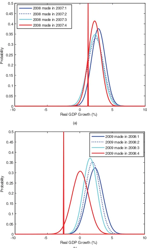
The first issue is whether a simple reduced-form model was better than the SPF in catching up with the financial crisis. Alessi et al. (2014) noted that “at the outset of the global financial cri-sis we note that the cross-section of the SPF and the FRBNY scenarios were well aligned. This completely changes in 2008 and 2009. The cross-section of SPF is overall more optimistic than the FRBNY. Gradually, as the U.S. economy started to
-100 -5 0 5 10
Figure 2. SPF density forecasts. Panel (a) Forecasts for 2008. Panel (b) Forecasts for 2009. Notes: The figure reports SPF densities forecasts for the following year’s real GDP growth. Dates are indicated in the legend. Realized GDP growth is depicted as a vertical line.
slowly recover over the next set of years we see that the SPF became less optimistic when measured against the range of out-comes considered in the simulated paths of the FRBNY models. (. . .) The FRBNY appears to be quicker than (. . .) the SPF in recognizing the downside risk of the crisis.”
Figure 2confirms Alessi et al.’s (2014) finding.Figure 2 re-ports SPF density forecasts for the following year’s real GDP growth; the realized GDP growth is also depicted as a vertical line. We plot SPF forecasts for 2008 (top panel) and 2009 (bot-tom panel) made in the quarters indicated in the legend. For example, the density labeled “2008 made in 2007:1” is the fore-cast made in 2007:1 for 2008, the density labeled “2008 made in 2007:2” is the forecast made in 2007:2 for 2008, and so forth. The figure shows that the SPF was sluggish in adjusting its fore-casts, and consistently overpredicted the target throughout 2008 and 2009.
-100 -5 0 5 10
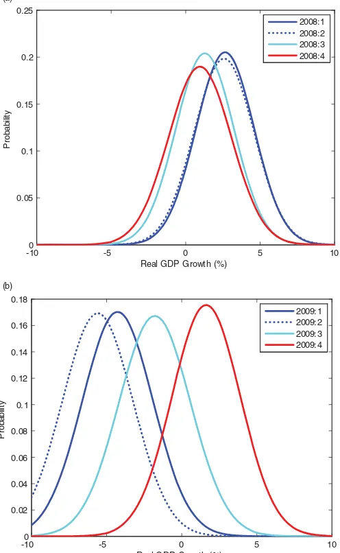
Figure 3. AR density forecasts. Panel (a) Forecasts for 2008 (var-ious quarters). Panel (b) Forecasts for 2009 (var(var-ious quarters). Notes: The figure reports AR densities forecasts for the following year’s real GDP growth. Dates are indicated in the legend. Realized GDP growth is depicted as a vertical line.
How fast would an AR model, instead, recognize the down-side risk of the crisis?Figure 3plots density forecasts in each quarter of 2008 and 2009 using the simple AR model. The den-sity labeled “2008:1” is the forecast made in 2007:4 for 2008:1; the density labeled “2008:2” is the forecast made in 2008:1 for 2008:2, and so forth. Note that the SPF produces forecasts for a target variable that is different from that of the AR model: the SPF focuses on predicting average GDP growth in the following year, whereas the AR model predicts annualized GDP growth starting the following quarter. However, we can compare the SPF forecast labeled 2009:4 (which was made in 2008:4 for 2009) with the AR forecast labeled 2009:1 (which was also made in 2008:4 for 2009:1, and is annualized). Note how the AR model forecasts a deeper recession for 2009:1 than the SPF; thus, the AR picks up the shift in the probability distribution of the output forecast already in late 2008, and by early 2009 it has already adjusted its forecasts. Even though the SPF and
the AR model produce forecasts for different variables, Figures 2 and3 show that the AR model was faster than the SPF in catching up with the signs of the crisis. This suggests that it might be interesting to evaluate the performance of the central banks’ density forecasts against those of simple reduced-form models to evaluate whether the former were faster than the latter in catching signs of the imminent recession.
3.2 Are Forecast Densities Correctly Specified?
Given that the AR forecasts adjust faster than the SPF to the crisis in real-time, we will focus on them in what follows. A traditional tool to evaluate the correct specification of density forecasts is the probability integral transform, or PIT. The PIT is the cumulative probability evaluated at the realized value of the target variable. It measures the ex-ante probability that one would have assigned, based on the forecast density, to observing a value less than the realized value. Diebold, Gunther, and Tay (1998) showed that, if the forecast density is correctly specified, the PIT is uniform with zero mean and unit variance, and it is independent and identically distributed. They proposed to test the correct specification of density forecasts by testing whether the PIT is uniform and uncorrelated. In what follows, we will apply these tests to the density forecasts of the AR model.
Test of Uniformity.Figure 4plots the empirical distribution of the PIT for one quarter-ahead density forecasts of annualized U.S. real GDP growth using the AR model. The empirical dis-tribution function closely resembles the disdis-tribution function of a standard uniform, thus pointing toward correct specification.
How different is the empirical distribution function from the theoretical (uniform) distribution? The literature has proposed several tests. For example, Corradi and Swanson (2006a,b) and Rossi and Sekhposyan (2013a) proposed tests to evaluate uni-formity by focusing on the empirical cumulative distribution function of the PIT. If the PITs were uniform, their empirical cumulative distribution function would resemble a 45-degree line. The difference between Corradi and Swanson (2006a,b)
Figure 4. Empirical distribution function of the PITs for the AR model. Notes: The figure plots the empirical distribution function of the PITs for the AR model. The dotted line represents the empirical distribution function of a standard uniform.
Figure 5. Uniformity test for the AR model (based on Rossi and Sekhposyan2013a). Notes: The figure plots Rossi and Sekhposyan’s (2013a) test statistic (solid line) together with its value under the null hypothesis (the 45-degree line) and 95% confidence bands (dotted lines).
and Rossi and Sekhposyan (2013a) is the way they handle pa-rameter estimation error: the former allow for a large estimation window size whereas the latter assume a fixed estimation win-dow size.
Figure 5shows the empirical cumulative distribution function of the PIT of the autoregressive model forecasts (dark, solid line) together with the uniform cumulative distribution function (45-degree, solid line) and 95% confidence bands based on the test proposed by Rossi and Sekhposyan (2013a), depicted as dotted lines. The test rejects when the empirical cumulative distribution function is outside the confidence bands. Clearly, there is no evidence of misspecification.
Tests of Serial Correlation.One could also test the correct specification of density forecasts by evaluating the serial corre-lation properties of the PITs. The Ljung–Box test applied to the de-meaned PITs has ap-value of 0.12 and the same test applied to the variance of the PITs has ap-value of 0.22. Clearly, there is no evidence of serial correlation in the PITs of the AR model, which increases our confidence in its correct specification.
4. CONCLUSION
The article by Alessi et al. (2014) has convincingly shown that the FRBNY density forecasts were faster than the SPF in recognizing the signs of the imminent financial crisis in real time, and that the use of financial indicators would have helped in further improving the density forecasts. The latter analysis can be thought of as an example of a forecast rationality test.
This comment has investigated a few examples of alternative tests that could complement the analysis in Alessi et al. (2014). By applying some of these techniques, I uncover empirical evi-dence against forecast unbiasedness of the ECB forecasts during the financial crisis. Also, I find that an AR model would have been faster than the SPF in catching up with the signs of the crisis.
It would be interesting to use these and other techniques to evaluate the correct specification of both the ECB and the FRBNY point and density forecasts to shed further light on their properties.(For example, it might be interesting to test the stability of the correct specification of the forecast densities. Such test would be useful to evaluate whether the financial crisis has introduced misspecification in the forecast densities. The analysis could be conducted, for example, by using the test for the correct specification of forecast densities robust to the presence of instabilities in Rossi and Sekhposyan (2013b). In addition, Giacomini and Rossi (2009) proposed tests for fore-cast breakdowns that could be used to investigate whether there was a breakdown in forecasting ability during the financial cri-sis. Giacomini and Rossi (2010) proposed tests to compare the predictive ability of competing forecasting models over time, when researchers suspect the relative predictive ability of the models might have changed over sub-periods. These techniques and several others are reviewed in Rossi (2013).)
ACKNOWLEDGMENT
I am grateful to S. Khan for organizing the special JBES session at the 2014 AEA Meetings, and T. Sekhposyan and G. Ganics for comments.
REFERENCES
Christoffel, K., Coenen, G., and Warne, A. (2010), “Forecasting With DSGE Models,” Discussion Paper N0. 1185, European Central Bank, Frankfurt am Main, Germany. [510]
Corradi, V., and Swanson, N. R. (2006a), “Bootstrap Conditional Distribution Tests in the Presence of Dynamic Mis-specification,”Journal of Economet-rics, 133, 779–806. [512]
——— (2006b), “Predictive Density Evaluation,” inHandbook of Economic Forecasting, eds. G. Elliott, C. Granger, and A. Timmermann, Elsevier, pp. 197–284. [512]
Diebold, F. X., Gunther, T. A., and Tay, A. S. (1998), “Evaluating Density Forecasts with Applications to Financial Risk Management,”International Economic Review, 39, 863–883. [512]
Edge, R. M., and G¨urkaynak, R. S. (2010), “How Useful Are Estimated DSGE Model Forecasts for Central Bankers?,” Brookings Papers on Economic Activity, 41, 209–259. [510]
Edge, R. M., G¨urkaynak, R. S., and Kisacikoglu, B. (2013), “Judging the DSGE Model by Its Forecast,” mimeo, Bilkent University and the Federal Reserve Board. [510]
Edge, R. M., Kiley, M. T., and Laforte, J. P. (2010), “A Comparison of Forecast Performance Between Federal Reserve Staff Forecasts, Simple Reduced-form Models, and a DSGE Model,”Journal of Applied Econometrics, 25, 720–754. [510]
Faust, J., and Wright, J. (2009), “Comparing Greenbook and Reduced Form Forecasts Using a Large Real-Time Dataset,”Journal of Business and Eco-nomic Statistics, 27, 468–479. [510]
Giacomini, R., and Rossi, B. (2009), “Detecting and Predicting Forecast Break-downs,”The Review of Economic Studies, 76, 669–705. [513]
——— (2010), “Forecast Comparisons in Unstable Environments,”Journal of Applied Econometrics, 25, 595–620. [513]
G¨urkaynak, R. S., Kisacikoglu, B., and Rossi, B. (2013), “Do DSGE Models Forecast More Accurately Out-of-Sample than VAR Models?” inAdvances in Econometrics: VAR Models in Macroeconomics. New Developments and Applications(Vol. 31), eds. T. Fomby, L. Kilian, and A. Murphy, Bingley, UK: Emeral Group Publishing Editor. [510]
Mincer, J., and Zarnowitz, V. (1969), “The Evaluation of Economic Forecasts,” inEconomic Forecasts and Expectations, ed. J. Mincer, New York: National Bureau of Economic Research, pp. 81–111. [510]
Patton, A., and Timmermann, A. (2012), “Forecast Rationality Tests Based on Multi-Horizon Bounds,”Journal of Business and Economic Statistics, 30, 1–17. [510]
Romer, C. D., and Romer, D. H. (2000), “Federal Reserve Information and the Behavior of Interest Rates,”The American Economic Review, 90, 429–457. [510]
Rossi, B. (2013), “Advances in Forecasting Under Model Instability,” in Hand-book of Economic Forecasting, eds. G. Elliottand A. Timmermann, (Vol. 2B), pp. 1203–1324, Amsterdam: Elsevier Publications. [513]
Rossi, B., and Sekhposyan, T. (2011), “Forecast Optimality Tests in the Presence of Instabilities,” mimeo, Duke University. [510]
——— (2013a), “Alternative Tests for Correct Specification of Conditional Forecast Densities,” mimeo, Universitat Pompeu Fabra and Texas A&M. [512,513]
——— (2013b), “Conditional Predictive Density Evaluation in the Presence of Instabilities,”Journal of Econometrics, 177, 199–212. [513]
West, K. D., and McCracken, M. W. (1998), “Regression-Based Tests of Predictive Ability,” International Economic Review, 39, 817– 840. [510]
Rejoinder
Lucia A
LESSIEuropean Central Bank, 60311 Frankfurt am Main, Germany ([email protected])
Eric G
HYSELSDepartment of Finance, Kenan–Flagler Business School, and Department of Economics, University of North Carolina at Chapel Hill, Chapel Hill, NC 27599 ([email protected])
Luca O
NORANTEJoint Modeling Project, Central Bank of Ireland, Central Bank of Ireland, Dublin, Ireland, and formerly, European Central Bank, 60311 Frankfurt am Main, Germany ([email protected].)
Richard P
EACHMacroeconomic and Monetary Studies Function, Federal Reserve Bank of New York, New York, NY 10045 ([email protected])
Simon P
OTTERMarkets Group, Federal Reserve Bank of New York, New York, NY 10045 ([email protected])
1. THE USEFULNESS OF HIGH-FREQUENCY
FINANCIAL DATA
Almost all the discussants comment on our findings regarding the usefulness of high-frequency financial market indicators as possible sources of forecast improvements. Hubrich and Man-ganelli as well as Kenny refer to Banbura et al. (2013) who reported that daily financial data do not significantly improve the nowcasting performance of factor-based models for U.S. GDP growth. Beyond the methodological differences between MIDAS regression and the dynamic factor state-space model discussed in detail notably by Andreou, Ghysels, and Kourtel-los (2013), it is worth noting that Banbura et al. only used a handful of daily financial assets, namely the S&P 500 stock price index, short- and long-term interest rates, the effective exchange rate, and the price of oil. These series are typically not very informative when trying to retrieve information from financial markets. The discussion by Scotti indeed highlights the fact that series which are incorporated in stress indices, such as credit default swaps, LIBOR-OIS spreads, corporate bond credit spreads, CDS data, VIX, etc. (series also included in the analysis by Andreou, Ghysels, and Kourtellos (2013)) tell a different story as illustrated by the analysis of a small Bayesian VAR model she reports in her discussion. Along these lines, Scotti notes that it might be easier to construct informa-tive high-frequency indices and use these directly in a MIDAS regression, as opposed to the forecast combination approached
used in our article. This point is well taken, and in fact one of the interesting series, besides the stress index, is the ADS index con-structed by Boragan Aruoba, Frank Diebold, and Chiara Scotti (see Aruoba, Diebold, and Scotti (2009)). Andreou, Ghysels, and Kourtellos (2013) reported empirical findings which shed some light on this, namely they compare a setting where prin-cipal components are extracted from a panel of high-frequency data and subsequently used in a MIDAS regression versus a set-ting where single high-frequency ADL-MIDAS regressions are used with the same high-frequency data which are then subse-quently aggregated through forecast combinations. The results indicate that the differences are minor. Practically, of course it may be very useful to rely on some well-chosen index series, such as the stress index or the ADS series.
It is perhaps worth reiterating that we believe that the virtues of our approach can be summarized in one word: parsimony. The MIDAS regression-based framework incorporates addi-tional and timely information, and hedge against major mis-takes by using model averaging techniques, thereby circum-venting the curse of dimensionality. Each MIDAS regression focuses on a single high-frequency indicator, and uses a parsi-monious parameterization. In the second step, model averaging
© 2014American Statistical Association Journal of Business & Economic Statistics
October 2014, Vol. 32, No. 4 DOI:10.1080/07350015.2014.958920