Pathological Outcomes of Observational L

PATHOLOGICAL OUTCOMES OF OBSERVATIONAL LEARNING

BY LONES SMITH AND PETER SøRENSEN1

This paper explores how Bayes-rational individuals learn sequentially from the discrete actions of others. Unlike earlier informational herding papers, we admit heterogeneous preferences. Not only may type-specific ‘‘herds’’ eventually arise, but a new robust possibility emerges: confounded learning. Beliefs may converge to a limit point where history offers no decisive lessons for anyone, and each type’s actions forever nontrivially split between two actions.

To verify that our identified limit outcomes do arise, we exploit the Markov-martingale character of beliefs. Learning dynamics are stochastically stable near a fixed point in many Bayesian learning models like this one.

KEYWORDS: Informational herding, cascades, martingale, Markov process, stochastic stability.

1. INTRODUCTION

SUPPOSE THAT A COUNTABLE NUMBER OF INDIVIDUALS each must make a

once-in-a-lifetime binary decisionᎏencumbered solely by uncertainty about the state of the world. If preferences are identical, there are no congestion effects or network externalities, and information is complete and symmetric, then all ideally wish to make the same decision.

But life is more complicated than that. Assume instead that the individuals must decide sequentially, all in some preordained order. Suppose that each may condition his decision both on his endowed private signal about the state of the world and on all his predecessors’ decisions, but not their hidden private signals.

Ž .

The above framework was independently introduced in Banerjee 1992 and

Ž . Ž .

Bikhchandani, Hirshleifer, and Welch 1992 hereafter, simply BHW . Their common conclusion was that with positive probability an ‘‘incorrect herd’’ would arise: Despite the wealth of available information, after some point, everyone might just settle on the identical less profitable decision.

In this paper, we study more generally how Bayes-rational individuals sequen-tially learn from the actions of others. This leads to a greater understanding of

1

This second revision is based on numerous suggestions from three referees and the Editor. We have also benefited from seminars at MIT, Yale, IDEI Toulouse, CEPREMAP, IEA Barcelona, Pompeu Fabra, Copenhagen, IIES Stockholm, Stockholm School of Economics, Nuffield College, LSE, CentER, Free University of Brussels, Western Ontario, Brown, Pittsburgh, Berkeley, UC San Diego, UCLA, UCL, Edinburgh, Cambridge, Essex, and IGIER. We wish also to specifically acknowledge Abhijit Banerjee, Kong-Pin Chen, Glenn Ellison, John Geanakoplos, David Hirsh-leifer, David Levine, Preston McAfee, Gerhard Orosel, Thomas Piketty, Ben Polak, and Jorgen¨ Weibull for useful comments, and Chris Avery for early discussions on this project. All errors remain our responsibility. Smith and Sørensen respectively acknowledge financial support for this work from the National Science Foundation and the Danish Social Sciences Research Council.

individual deviates. What then could Mr. one million and two conclude? First, he could decide that his predecessor had a more powerful signal than everyone else. To capture this, we generalize the private information beyond discrete signals, and admit the possibility that there is no uniformly most powerful yet nonrevealing signal. Second, he might believe that the action was irrational or an accident. We thus add noise to the herding model. Third, he might decide that different preferences provoked the contrary choice. On this score, we consider the model with multiple types, and find that herding is not the only possible ‘‘pathological’’ longrun outcome: We may converge to an informational pooling equilibrium where history offers no decisive lessons for anyone, and everyone must forever rely on his private signal.

Ž .

The paper is unified by two natural questions: i What are the robust long-run outcomes of learning in a sequential entry model with observed

Ž .

actions? ii Do we in fact settle on any one? Our inquiry is focused through the two analytic lenses of convergence of beliefs and convergence of actionsᎏeither in frequency or, more strongly, with herds. BHW introduced the terminology of a cascade for an infinite train of individuals acting irrespective of the content of their signals. With a single rational type and no noiseᎏhenceforth, the herding modelᎏindividuals always settle on an action, starting a herd. Yet the label ‘‘cascades literature’’ is appropriate outside BHW’s discrete signal world. Among our simplest findings is that barring discrete signals, cascades need not arise: No decision need ever be a foregone conclusion even during a herd. With these two notions decoupled, the analysis is richer, and it suggests why we must admit a general signal space, and adopt a stochastic process approach. For instance, Theorem 1 shows that learning is incomplete exactly when private signals are uniformly bounded in strength. By Theorem 3, then and only then can bad herds possibly arise in the herding model.

statistical inferences may be drawn about any given individual. Taste diversity with hidden preferences describes numerous cited motivating examples of herd-ing in the literature, such as restaurant choice, or investment decisions. This twist yields our principal new economic findings. The standard herding outcome

Ž

is robust to individuals having identical ordinal but differing cardinal von

.

Neumann Morgenstern preferences. With multiple rational preference types, not all ordinally alike, an interior rational expectation dynamic steady-state robustly emerges: It may be impossible to draw any clear inference from history even while it continues to accumulate privately-informed decisions. Further, this incomplete learning informational pooling outcome exists even with unbounded beliefs, when an incorrect herd is impossible.

Let us fix ideas and illustrate thisconfounded learning outcome with a possibly familiar example. Suppose that on a highway under construction, depending on how detours are arranged, those going to Houston should take either the high or

Ž .

low off-ramps in states H and L, with the opposite for those headed toward Dallas. If 70% are headed toward Houston, then absent any strong signal to the contrary, Dallas-bound drivers should take the lane ‘‘less traveled by.’’ This yields two separating herding outcomes: 70% high or 70% low, as predicted by armchair application of the herding logic. But another possibility may arise. As the chance q that observed history accords state H rises from 0 to 1, the probability that a Houston driver takes the high road gradually rises from 0 to 1,

Ž . Ž .

and conversely for Dallas drivers. Thus, the fraction ␺_H q and ␺_L q in the right lane in states H,Leach rise from 0.3 to 0.7, perhaps nonmonotonically so. If for some q, a random car is equilikely in states H and L to go high, or

Ž . Ž .

␺H q _s␺L q, then no inference can be drawn from additional decisions: Learning then stops. While existence of such a fixed point is not clear, Theorems 1 and 2 prove that confounding outcomes co-exist with the cascade possibilities, for nondegenerate models.

Our confounded learning outcome is generic when two types have opposed preferences, assuming uniformly bounded private signals. With unbounded signals, it emerges for sufficiently strongly opposed von Neumann Morgenstern

Ž .

preferences, and not too unequal population frequencies. In either case,␺_H q

Ž . Ž . Ž .

)␺_L q for small enough q, and ␺_H q -␺_L q for large enough q.

Two stochastic processes constitute the building blocks for our theory: the

Ž

public likelihood ratio is a conditional martingale, and the vector action taken,

.

likelihood ratio a Markov chain. Martingale and Markovian methods are standard methods for ruling out potential limit outcomes of learning. But our major technical contribution concerns their stability: Given multiple limit be-liefs, must we converge upon any given one? How can we rule in any limit? For instance, even if our highway driving confounding outcome robustly exists, must we converge upon it? Theorem 4 gives a simple easily checked condition for the

Ž .

published instance. More recently, Piketty 1995 has found confounded learning outcomes in a model where individuals passively learn about social mobility parameters.

Section 2 gives a common framework for the paper. Section 3 illustrates our findings in three examples. We then proceed along two technical themes. First, via Markov-martingale means, Section 4 describes the action and belief limits; the confounding outcome is the key finding here. Next, Section 5 motivates and states the stability result, and as an application, shows when a long-run outcome arises. Extension to finitely many states is addressed in the conclusion; there we also describe extensions of the paper, as well as some related literature. More detailed proofs and some essential math results are appendicized.

2. THE COMMON FRAMEWORK

2.1. The Model

States. There are S_s2 payoff-relevant states of the world, the high state

s_sH and the low state s_sL. As is standard, there is a common prior

Ž . Ž .

beliefᎏwithout loss of generality, a flat prior Pr H _sPr L _s1_r2. Our results extend to any finite number S of states, but at significant algebraic cost, and so

Ž .

this extension is addressed in the conclusion §6.1 .

Pri¨ate Beliefs. An infinite sequence of individuals n_s1, 2, . . . enters in an exogenous order. Individual n receives a random pri¨ate signalabout the state

Ž .

of the world, and then computes via Bayes’ rule his pri_¨ate belief pn_g 0, 1 that

4

the state is H. Given the state s_g H,L, the private belief stochastic process

²_p :_{is i.i.d, with conditional c.d.f. F}s_{. These distributions are sufficient for the} n

state signal distribution, and obey a joint restriction implicit below. The curious reader may jump immediately to Appendix A, which summarizes this develop-ment, and explores the results we need.

We assume that no private signal, and thus no private belief, perfectly reveals the state of the world: This ensures that FH_,FL _{are mutually absolutely}

Ž .

continuous, with common support, say supp F . Thus, there exists a positive,

L H _{Ž . Ž .}

finite Radon-Nikodym derivative f_sdF _rdF : 0, 1 ª 0,⬁. And to avoid trivialities, we assume that some signals are informative: This rules out f_s1 almost surely, so that FH _{and F}L _{do not coincide. When F}s _{is differentiable}

Ž_s . s

sL,H , we shall denote its derivative by f .

Ž Ž .. w x w x

The convex hull co supp F ' b,b _: 0, 1 plays a major role in the paper. Note that b-1_r2-b as some signals are informative. We call the private

Ž Ž .. w x

Indi_¨idual Types and Actions. Every individual makes one choice from a finite

4

action menu MM_{s 1, . . . ,M , with MG2 actions. We allow for heterogeneous} preferences of successive individualsᎏthe only other random element. A model with multiple but observable types is informationally equivalent to a single preference world. So assume instead that all types are private information. There are finitely many rational types t_s1, . . . ,T with different preferences. Let

␭t _{be the known proportion of type t.}

We also introduce M crazy types. Crazy type m arrives with chance ␬m_G0, and always chooses action m. One could view these as rational types with state independent preferences, and unlike everyone else, a single dominant action.

Ž .

We assume a positive fraction ␬_s1_y ␬1_q⭈⭈⭈_q␬M )0 of payoff-motivated rational individuals. Rational and crazy types are spread i.i.d. in sequence, and

² :

independently of the belief sequence pn .

4 s_{Ž .}

Payoffs. In state s_g H,L, each rational type t earns payoff u mt from

Ž t _.

action m for precision, sometimes a_m , and seeks to maximize his expected

Ž .

payoff. For each rational type, M_G M_tG2 actions are not weakly dominated, and generically no one action is optimal at just one belief, and no pair of actions

Ž .

provides identical payoffs in all states. Each type t thus has S_s2 extreme actions, each strictly optimal in some state. The other M_ty2 insurance actions

are each taken at distinct intervals of unfocused beliefs.

w x

Given a posterior belief r_g0, 1 that the state is H, the expected payoff to

H_{Ž . Ž .} L_{Ž .}

type t of choosing action mis ru_t m _q 1_yr u_t m . Figure 1 depicts the next summary result.

w x t t

LEMMA 1: For each rational type t, 0, 1 partitions into subinter¨als I1, . . . ,IMt

touching at endpoints only, with undominated action m_gMM_:MM _{optimal exactly} t

for beliefs r_gIt_. m

With multiple types, we must introduceT labels for every action. Permuting M

M_{t, we order rational type t’s actions a1}t_{, . . . ,a}t_{M by relative preference in state} t

H, with at _{most preferred. So to be clear, if we order actions from least to most} M

preferred by type t in state H, then action m has rank ␰_s␰t _{if m}

sat_{. By}

m ␰

m m

Ž t t _.Ž t⬘ t⬘_.

over actions m and m⬘ if ␰m_y␰m⬘ ␰m_y␰m⬘ -0ᎏi.e. their ordinal prefer-ences for them in state H, and thus in state L, are reversed. With just a single rational type, we suppress t superscripts, and likewise strictly order belief thresholds as 0_sr0-r1-⭈⭈⭈-rM_s1.

2.2. The Indi¨idual Bayesian Decision Problem

Before acting, every rational individual observes his type t, his private belief

p, and the entire ordered action history h. His decision rule then maps pand h

into an action. We look for a Bayesian equilibrium, where everyone knows all

s_{Ž .}

decision rules, and can compute the chance␲ h of any history hin each state

Ž . H_{Ž . Ž} H_{Ž .} L_{Ž ..}

s. This yields a public belief q h _s␲ h_r␲ h _q␲ h that the state is H, i.e. the posterior given h and a neutral private belief p_s1_r2. Applying Bayes rule again yields the posterior belief r in terms of q and p:

H_{Ž .}

p␲ h pq

Ž .1 r_sr pŽ ,q._{s H L s} .

Ž . Ž .

Ž . Ž . Ž . pq_q 1_yp 1_yq

p␲ h _q 1_yp ␲ h

As belief q is informationally sufficient for the underlying history data h, we now suppress h.

Ž .

Since the right hand side of 1 is increasing in p, there are pri¨ate belief

t_{Ž .} t_{Ž .} t _{Ž .}

thresholds0_sp q0 _Fp q1 _F⭈⭈⭈_FpM q _s1, such that typetoptimally chooses

t _Ž t _{Ž .} t_{Ž .x}

action am iff his private belief satisfies pg pmy1 q ,pm q , given the earlier

t_{Ž .}

tie-break rule. Furthermore, each threshold p_m q is decreasing in q. A type-t

t _{Ž . w} t _{Ž .} t_{Ž .x4}

cascade set is the set of public beliefs J_ms q_Nsupp F _: p_my1 q,p_m q . So

t _Ž t_{. Ž .} t

type t a.s. takes action a_m for any q_gint J_m , since the posterior r p,q _gI_m

for all p. It follows that any cascade set lies inside the corresponding action

t _Ž t_. t

basin, so that J_m:int I_m . For if all private beliefs yield action a_m, then so must the neutral belief.

Ž .

As is standard, call a property generic resp. nondegenerate or robust if the

Ž

subset of parameters for which it holds is open and dense resp. open and

.

nonempty .

LEMMA2: For each action amt and type t, Jmt is a possibly empty inter¨al. Also,

t t t t t

Ž .a with bounded pri¨ate beliefs, J1_sw0,qx and JM_tswq, 1x for some 0-q

-t

q-1;

Ž . t ₄ t ₄ t

b with unbounded pri¨ate beliefs, J1_s 0 , JM_ts 1 , and all other Jm are empty;

Ž . s t

t

The appendicized proofs of Lemma 2 a, b are also intuitive: With bounded private beliefs, posteriors are not far from the public belief q; so for q near enough 0 or 1, or well inside an insurance action basin, all private beliefs lead to

Ž .

the same action. With unbounded beliefs, every public belief q_g 0, 1 is swamped by some private beliefs. Next, given the continuous map from payoffs

² s_{Ž .: ²} t_{: Ž . Ž .}

The paper requires some more notation. Define Jt sJt

jJt

j⭈⭈⭈_jJt _{. A type t}

1 2 M_t

is acti¨e when choosing at least two actions with positive probability. A cascade

arisesᎏeach type’s action choice is independent of private beliefsᎏfor public beliefs strictly inside J_sJ1_lJ2_l⭈⭈⭈_lJT: however, with unbounded beliefs,

4 4 H t

there are two cascade beliefs: qgJs 0 j 1 . We put J 'FtJMt, namely where each type t cascades on the action at

, which is optimal in state H.

Mt

Similarly, we define JL _{for state L.}

2.3. Learning Dynamics

Let qn be the public belief after Mr. n chooses action mn. It is well-known

² :⬁ _{Ž < .}

that q _n obeys an unconditional martingale, EE _{q q sq , and hence}

s1

n nq1 n n

almost surely converges to a limit random variable. While we could in principle employ this posterior belief process, we care about the conditional stochastic

Ž .

properties in a given state H. Thus, the public likelihood ratio l_n' 1_yq_{n r}q_n

that the state is L versus H offers distinct conceptual advantages, and saves

² :

time, as it conditions on the assumed true state. The likelihood process l_n

similarly will be a convergent conditional martingale on state H.

We then have likelihood analogues of previous notation, now barred: private

t_{ŽŽ . .} t_{Ž .} t t

Likelihood ratios ln ns1 are a stochastic process, described by l0_s1 as

.

q0_s1_r2 and transitions

t t s t s t

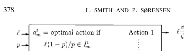
FIGURE2.ᎏIndividual black box. Everyone bases his decision on both the public likelihood ratio

t _Ž t _{< .}

land his private belief p, resulting in his action choiceam with chance␺ amL,l, and a likelihood

Ž t _. t

ratio ␸ a_m,l to confront successors. Typet takes action a_m if and only if his posterior likelihood

t t t

Ž . w x

l1yp_rplies in the interval Im, where I1, . . . ,IMt partition 0,⬁.

T

t t

Ž .4 ␺Žm s< ,l._s␬m_q␬

_Ý

␭␳ Žm s< ,l.,

ts1

Ž .5 ␸Žm,l._sl␺Žm L< ,l._r␺Žm H< ,l..

t_{Ž < .}

Here, ␳ m s,l is the chance that a rational type t takes action m, given l, and

t

4

the true state sg H,L. So the cascade set Jm is the interval of likelihoods l

t_Ž t _{< .} t_Ž t _{< .}

yielding ␳ am H,l _s␳ am L,l _s1. Faced with ln, Mr. n takes action mn

Ž < . Ž .

with chance ␺ m sn ,ln in state s, whereupon we move to lnq1_s␸ mn,ln .

Ž . Ž .

Figure 2 summarizes 3᎐ 5 .

² :

Our insights are best expressed by considering the pair mn,ln as a

discrete-w .

time, time-homogeneous Marko¨ process on the state space MM_{= 0,⬁. Given} ²m_n,l_n:, the next state is²m_nq1,␸Žm_nq1,l_n.:with probability␺Žm_nq1<s,l_n.in

² :

state s. Since l_n is a martingale, convergence to any dead wrong belief almost surely cannot occur, since the odds against the truth cannot explode. In summary we have the following lemma.

Ž . ² :

LEMMA 3: a The likelihood ratio process l_n is a martingale conditional on

state H.

Ž .b Assume state H. The process ² :ln con¨erges almost surely to a r.¨., l⬁_s

Ž . w . Ž .

limnª⬁ln,with supp l⬁ _: 0,⬁.So fully incorrect learning lnª⬁ almost surely cannot occur.

Ž . ² :

PROOF: See Doob 1953 for the martingale character of ln . Convergence

follows from the Martingale Convergence Theorem for nonnegative, perhaps

Ž Ž . .

unbounded, random variables Breiman 1968 , Theorem 5.14 ; Bray and Kreps

Ž1987 prove this with public beliefs.. Q.E.D.

Ž .

² :

Belief convergence then forces action con_¨ergence: m_n settles down in

Ž . Ž .

frequency, or lim_nª⬁N m_{n r}n exists for all m, where N m_n '噛 m_ksm,

4

k_Fn.

COROLLARY: Action con_¨ergence almost surely obtains,if Fs has no atoms.

Ž .

PROOF: Let ␧)0. Given belief convergence Lemma 3 , continuity of

Ž . Ž . Ž .

⌿ m_Ns,l , and the law of motion 4 , the chance ␣_m n that action m is chosen

Ž . Ž .

almost surely converges, say␣m n ª␣m. Thus,␣m n _F␣m_q␧ for large n, and

Ž . Ž .

so lim supnª⬁N nm _rn_F␣m_q␧. Similarly, lim infnª⬁N nm _rn_G␣m_y␧. Since

Ž .

␧)0 is arbitrary, limnª⬁N nm _rn_s␣m. Q.E.D.

The literature has so far focused on two more powerful convergence notions. As noted, a cascade means ln_gJ, or finite time belief convergence. Since every later rational type’s action is dictated by history, this forces a herd, where rational individuals of the same type all act alike. By corollary, the weaker action convergence obtains. We also need the weaker notion of a limit cascade, or eventual belief convergence to the cascade set: l_⬁gJ.

3. EXAMPLES

3.1. Single Rational Type

Consider a simple example, with individuals deciding whether to ‘‘invest’’ in or

Ž .

‘‘decline’’ an investment project of uncertain value. Investing action m_s2 is

Ž .

risky, paying off u)0 in state Hand_y1 in state L; declining action m_s1 is a neutral action with zero payoff in both states. Indifference prevails when

Ž . Ž . Ž .

0_sru_y 1_yr , so that r_s1_r1_qu. Thus, equation 1 defines the private

Ž . Ž .

belief threshold p l _sl_r u_ql .

Ž .

A. Unbounded Beliefs Example. Let the private signal ␴_g 0, 1 have

state-H_{Ž .} L_{Ž . Ž .}

contingent densities g ␴ _s2␴ and g ␴ _s2 1_y␴ ᎏas in the left panel of

Ž . Ž .

Figure 3. With a flat prior, the private belief p_sp ␴ then satisfies 1_yp_rp_s

L_{Ž .} H_{Ž . Ž .}

g ␴ _rg ␴ _s 1_y␴ _r␴ by Bayes’ rule, and has the same conditional

densi-H_{Ž .} L_{Ž . Ž .} H_{Ž .} 2 L_{Ž .}

ties f p '2pand f p '2 1_yp, and c.d.f.’s F p _sp and F p _s2p

2 _{Ž . w x}

yp . So supp F _s 0, 1 , and private beliefs are unbounded; the cascade sets

4 4

collapse to the extreme points, J1_s ⬁, J2_s 0 .

Ž . Ž .

FIGURE4.ᎏContinuation and cascade sets. Continuation functions for the examples: unbounded

Ž . Ž . Ž .

private beliefs left , and bounded private beliefs right with ␬1_s␬2_s1r10 and without noise Ždashed and solid lines . The stationary points are where both arms hit the diagonal as with noise ,. Ž .

Ž

or where one arm is taken with zero chance l_s0 orl_s⬁in the left panel;l_F2u_r3 orl_Guin the .

right panel without noise . With crazy types the discontinuity vanishes, and isolated deviations no longer have drastic consequences. Graphs here and in Figure 5 were generated analytically with PostScript.

Figure 4 left panel , the only stationary finite likelihood ratio in state H is 0; the limit l_⬁of Lemma 3 is focused on the truth. As the suboptimal action 1 lifts

ln_G2u, an infinite subsequence of such choices would preclude belief

conver-Ž .

gence. Hence, there must be action convergence i.e. a herd .

L_{Ž .}

B. Bounded Beliefs Example. Let private signals have density g ␴ _s3_r2_y␴

Ž . Ž . The likelihood ratio converges by Lemma 3, so that J_1jJ₂ contains all possible

Ž .

stationary limits, as in Figure 4 right panel . A herd on action 1 or 2 must then

Ž < .

Here, we may strongly conclude that each limit outcome 2u_r3 and 2uarises

In contrast to BHW, if public beliefs are not initially in a cascade set, they never enter one. This holds even though a herd always eventually starts.

Ž . Ž .

Visually, it is clear that l_ng 2u_r3, 2u for all n if l_0g 2u_r3, 2u . This also

Ž .

follows analytically: If ln-2u, then lnq1s␸ 1,ln sur2q3lr4-ur2q3ur2

s2utoo. So herds must arise even though a contrarian is never ruled out. This

Ž .

result obtains whenever continuation functions ␸ i,⭈ are always increasing. For

² :

then ln never jumps into the closed set J1_jJ2, starting a cascade. Monotonic-ity is crucially violated in BHW’s discrete signal world.

C. Bounded Beliefs Example with Noise. Suppose that a fraction of individuals randomly chooses actions. This introduction of a small amount of noise radically affects dynamics, as seen in the right panel of Figure 4. For since all actions are

Ž .

expected to occur, none can have drastic effects. Namely, each ␸ i,⭈ is now continuous near the cascade sets at l_s2u_r3 and l_s2u. Yet, the limit beliefs

Ž

are unaffected by the noise, contrary actions being deemed irrational and

.

ignored inside the cascade sets.

3.2. Multiple Rational Types

With multiple types, one can still learn from history by comparing proportions choosing each action with the known type frequencies. This inference intuitively should be fruitful, barring nongenericities. A new twist arises: Dynamics may lead to each action being taken with the same positive chance in all states, choking off learning. This incomplete learning outcome is economically different than herdingᎏinformational pooling, where actions do not reveal types, rather than the perfect separation that occurs with a type specific informational herd. Mathematically it is a robust interior sink to the dynamics.

Let us consider the driving example from the introduction. Posit that Houston

Žtype U, our ‘‘usual’’ preferences drivers should go high action 2 in state. Ž . H,

Ž . Ž .

low action 1 in state L, with the reverse true for Dallas typeV drivers. Going to the wrong city always yields zero, without loss of generality. The payoff vector

Ž . Ž .

of the Houston-bound is 0,u in state Hand 1, 0 in state L; for Dallas drivers,

Ž . Ž .

it is 1, 0 and 0,_¨ , where without loss of generality _¨Gu)0. So the prefer-ences are opposed, but not exact mirror images if ¨)u. Types U,V then

U_{Ž . Ž .}

respectively choose action 1 for private beliefs below p l _sl_r u_ql , and

V_{Ž . Ž .}

above p l _sl_{r ¨q}l .

Assume the same bounded beliefs structure introduced earlier. Assume we

U V

Ž < .

␺ 1H,l _s␭ _q␭ and

2l 2l

Ž3l_y2u. Ž3l_q2u. Ž2_¨yl.Ž2_¨ql.

U V

Ž < .

␺ 1L,l _s␭ _{2 q}␭ ₂ .

8l 8l

We are interested in a different fixed point depicted in Figure 5, where neither rational type takes any action for sure, and decisions always critically depend on

Ž . Ž < . Ž < .

private signals. The two continuations 5 then coincide:␺ 1H,l* _s␺ 1L,l*

Ž .

g 0, 1 , and actions convey no information:

U _{Ž .Ž .}

␭ 2¨yl 3l_y2¨

Ž .

s 'h l .

V _{Ž2u . Ž .} yl 3l_y2u ␭

Ž . Ž . Ž . U ¨

If _¨)u then h maps 2_¨r3, 2u onto 0,⬁, and h l* _s␭ _r␭ is solvable for any␭U_,␭V_.

² :

For this example, we can argue that with positive chance, the process ln

w x w x

tends to l* if it does not start in a cascade, i.e. in 0, 2u_r3 or 2¨,⬁. Since each

Ž . w x

likelihood continuation ␸ i,⭈ is increasing, if dynamics start in 2u_r3,l* or

wl*, 2¨x, they are forever trapped there. Assume l0_gŽ2u_r3,l* . Then. ² :ln is a bounded martingale that tends to the end-points; therefore, the limit l_⬁ places positive probability weight on both a limit cascade on l_s2u_r3 and convergence

FIGURE 5.ᎏConfounded learning. Based on our Bounded Beliefs Example, with ␭U s4r5, Ž < . Ž < .

u_s¨r2. In the left graph, the curves ␺ 1H,l and ␺ 1L,l cross at the confounding outcome

l*s8¨r9, where no additional decisions are informative. Atl*, 7r8 choose action 1, and strangely 7r8 lies outside the convex hull of ␭V_and␭U_{ᎏe.g., in the introductory driving example, more than}

to l_sl*. This example verifies that the latter fixed point robustly exists and is stable, but does not yet explain why.

4. LONG RUN LEARNING

4.1. Belief Con¨ergence: Limit Cascades and Confounded Learning

² :

A. Characterization of Limit Beliefs. That ln is a martingale in state H rules

Ž .

out nonstationary limit beliefs such as cycles , and convergence to incorrect point beliefs. Markovian methods then prove that with a single rational type, as in Section 3.1, limit cascades arise, or lnªJ. But with multiple rational types,

² :

the example in Section 3.2 exhibits another possibility: ln may converge to where each action is equilikely in all states. Then define the set K of confound

-ing outcomesas those likelihood ratios l*fJ satisfying

Ž .6 ␺Žm s< ,l*._s␺Žm H< ,l*. for all actions mand states s.

Observe that sincel*fJ, decisions generically depend on private beliefs. Yet decisions are not informative of beliefs, given the pooling across types. Also, history is still of consequence, or otherwise decisions would then generically be informative. Rather history is precisely so informative as to choke off any new inferences. The distinction with a cascade is compelling: Decisions reflect own private beliefs and history at a confounding outcome, whereas in a limit cascade, history becomes totally decisive, and private beliefs irrelevant.

Markovian and martingale methods together imply that with bounded private beliefs, fully correct learning is impossible. Only a confounding outcome or limit cascade on the wrong action are possible incomplete learning outcomes. Theo-rem 1 summarizes.

THEOREM1: Suppose without loss of generality that the state is H.

Ž .a With a single rational type,a not fully wrong limit cascade occurs: suppŽ .l_{⬁ :}

4

JR ⬁.

Ž .b With a single rational type, and unbounded pri¨ate beliefs, lnª0 almost surely.

Ž .c With T_G2 rational types with different preferences, only a limit cascade that

Ž . 4

is not fully wrong or a confounding outcome may arise: supp l_{⬁ :}J_jKR ⬁.

H

Ž .d With bounded pri¨ate beliefs, l_⬁gJRJ with positi¨e chance pro¨ided

H

l0fJ . Likewise, if l0/l*, no single confounding outcome l*arises almost surely.

Ž .e Fix payoff functions for all types,and a sequence of pri¨ate belief distributions

w x Ž . Ž .

with supports bk,bk ks1, 2, . . . . If bkª1 or bkª0 in state L , then the

H

chance of an incorrect limit cascade l_⬁gJRJ _¨anishes as kª⬁.

Ž . w .

s ior does not affect long run learning by rational individuals, as it is filtered out. Next, pick the least action mtaken in the limit by the rational type with positive

Ž .

chance i.e. for low enough private beliefs . Since private beliefs are informative

ŽLemma A.1 c ,Ž .. m is strictly more likely in state L than H, and is thus

ˆ

ˆ

ˆ

Ž < . Ž < .

informativeᎏunless ␳ m H,l _s␳ m L,l _s1. Hence, l_gJm. The Appendix analyzes the case of a discontinuous function ␸.

Ž . 4 Ž . done. Otherwise l_nFl-⬁ a.s. for all n. By the Dominated Convergence

² :

Theorem, the mean of the bounded martingale l_n is preserved in the limit:

H

cascade public likelihood ratio lk and the highest private belief bk yield the

t _Ž t_. t t_Ž t_. t

posterior r1, by Bayes rule: 1_yr1 _rr1_slk 1_ybk _rbk. So lkª⬁as bkª1, and

Ž .

thus␲kª0. In state L,␲kª0 as bkª0, and lkª0. Q.E.D.

Ž .

Observe how Part e makes sense of the bounded versus unbounded beliefs knife-edge, since there is a continuous transition from incomplete to complete learning.2

2 _{Ž .}

B. Robustness of Confounding Outcomes. Lemma 2 establishes the robustness of cascade sets. However, unlike cascade sets, the existence of confounding outcomes is not foretold by the Bayesian decision problem. They are only inferred ex post, and are nondegenerate phenomena. Fleshing this out, the

² s_{Ž .}

model parameters are the preferences and type_rnoise proportions u m_t ,

t_: S M TqMqT

␬_m,␭ , elements of the Euclidean normed space ⺢ . Genericity and robustness are defined with respect to this parameter set.

THEOREM2: Assume there are TG2 rational types.

Ž .a Confounding outcomes robustly exist, and are in¨ariant to noise.

Ž .b At any confounding outcome, at least two rational types are not in a cascade set.

Ž .c For generic parameters, at a confounding outcome, at most two actions are

Ž .

taken by acti_¨e rational types i.e. those who are not in a cascade.

Ž .d If belief distributions are discrete, confounded learning is nongeneric.

Ž .e With M)2 actions and unbounded beliefs, generically no confounding outcome exists.

Ž .f At any confounding outcome, some pair of types has opposed preferences.

Ž .g Assume M_s2 and some types with opposed preferences. With atomless bounded beliefs and T_s2, a confounded learning point exists generically, pro_¨ided both types are acti_¨e o_¨er some public belief range.With atomless unbounded beliefs

H_{Ž .} L_{Ž .}

and f 1 ,f 0 )0, a confounding point exists if the opposed types ha¨e suffi

-ciently different preferences.

Before the proofs, observe that while generically only two actions are active at

Ž Ž ..

any given confounding outcome Part c , nondegenerate models with M)2 actions still have confounding outcomes. For with bounded beliefs, only two actions may well be taken over a range of possible likelihoods l. Second, note that a confounding outcome is in one sense a more robust failure of complete learning than is an incorrect limit cascade, since it arises even with unbounded

Ž Ž ..

private beliefs Part g .

PROOF: Ž .

Proof of a: This has almost been completely addressed by the third example in Section 3, which is nondegenerate in the specified sense. Invariance to noise

Ž .

follows because shifting ␬_m identically affinely transforms both sides of 6 ,

Ž .

given 4 .

Ž . Ž .

Proof of b : By the proof of Theorem 1 a , if all but one rational type is in a

Ž .

cascade in the limit, then so is that type, given 6 . So at least two rational types are active.

Ž .

Proof of c : Consider the equations that a confounding outcome l* must solve. First, with bounded beliefs, some actions may never occur at l*. Assume that M0_FM actions are taken with positive probability at l*. Next, given the

M0 Ž < . M0 Ž < . Ž .

adding-up identityÝis1␺ m Hi ,l _sÝis1␺ m Li ,l _s1, 6 reduces to M0_y1

Ž < . Ž < .

␭ weights are perturbed.

Ž . Ž .

Proof of e : With unbounded private beliefs, for any lg 0,⬁, all Mactions

Ž .

are taken with positive chance. By Part c , confounding outcomes generically can’t exist.

Ž .

Proof of f : If actions 1 and 2 are taken at l*, and all types prefer m_s2 in state H, then m_s2 is good news for state H, whence l* could not be a confounding outcome.

Ž . w x

Proof of g : Consider an interval l,l between any two consecutive portions

Ž < .

of the cascade set J. The Appendix proves that under our assumptions,␺ 1H,l

Ž < . Ž < . Ž < .

exceeds ␺ 1L,l near l iff ␺ 1L,l exceeds ␺ 1H,l near l. Without signal atoms, both are continuous functions, and therefore must cross at some interior

Ž .

pointl*_g l,l . Q.E.D.

Ž Ž ..

For an intuition of why confounding points exist Theorem 2 g , consider our binary action Texas driving example depicted in Figure 5. By continuity, it

Ž < .

suffices to explain when one should expect the antisymmetric ordering ␺ 1L,l

Ž < . Ž . Ž .

c␺ 1H,l , respectively, for lsmall near l and large near l . The critical idea here is that barring a cascade, a partially-informed individual is more likely to

Ž

choose a given course of action when he is right than when he is wrong Lemma

.

A.1 .

Since Houston drivers wish to go high in state H, uniformly across public beliefs, more Houston drivers will go high in state H than in state L. The reverse is true for Dallas drivers. The required antisymmetric ordering clearly occurs if and only if most contrarians are of a different type near l than near l. With bounded beliefs, as in the example of §3.1B, this is true simply because a different type is active at each extreme, for generic preferences.

With unbounded beliefs, the above shortcut logic fails, as both types are active for all unfocused beliefs. The key economic ingredients for the existence

Ž .

of a confounding point are then i not too unequal population type frequencies,

Ž . Ž .

and ii sufficiently strongly opposed preferences by the rational types. To see i , assume the extreme case with rather disparate type frequencies, and nearly everyone Houston-bound. No antisymmetric ordering can then occur, as

Ž < . Ž < . Ž . Ž .

␺ 1L,l -␺ 1H,l for all l_g l,l . Next, condition ii ensures that the two types’ action basins for opposing actions grow, and contrarians of each typeᎏthose whose private beliefs oppose the public beliefᎏincrease as we approach one extreme, and decrease as we approach the other, in opposition.

To illustrate the intuition in an unbounded beliefs variant of the driving

Ž Ž ..

U V _Ž U V

for u_r¨c␭ _r␭ _c¨ru. In words, type frequencies are not too far apart ␭ _r␭

.

not too big or smallᎏand given their disparity, preferences are sufficiently

Ž .

strongly opposed u_r¨ big or small enough .

4.2. The Traditional Case: Herds with a Single Rational Type and No Noise

We have already argued that actions converge in frequency. Without noise, this can be easily strengthened. After any deviation from a potential herd, or finite string of identical actions, an uninformed successor will necessarily follow suit. In other words, the public belief has radically shifted. As in Section 3, this logic proves that herds arise.

THEOREM3: Assume a single rational type and no noise. Ž .a A herd on some action will almost surely arise in finite time.

Ž .b With unbounded pri¨ate beliefs,indi¨iduals almost surely settle on the optimal action.

Ž .c With bounded pri¨ate beliefs, absent a cascade on the most profitable action from the outset, a herd arises on another action with positi¨e probability.

Ž . Ž .

PROOF: Part a follows from the convergence result of Theorem 1 a and the following O_¨erturning Principle: If Mr. n chooses any action m, then before

n_q1 observes his own private signal, he should find it optimal to follow suit because he knows no more than n, who rationally chose m. To wit, l_nq1gI_m

after n’s action, and a single individual can overturn any given herd. The

Ž .

Appendix analytically verifies this fact. From Lemma 2, J_m;int I_m , so that

Ž . Ž .

when supp l_{⬁ :}J_m, eventually l_ngint I_m , precluding further overturns.

Ž . Ž . Ž . Ž . Ž .

Finally, Parts b and c are corollaries of Part a and Theorem 1 b and d .

Q.E.D.

This characterization result extends the major herding finding in BHW to

Ž

general signals and noise. BHW also handled several states, addressed here in

.

§6.1 . The analysis of BHWᎏwhich did not appeal to martingale methodsᎏonly succeeded because their stochastic process necessarily settled down in some stochastic finite time. Strictly bounded beliefs so happens to be the mainstay for their bad herds finding. Full learning doesn’t require the perfectly revealing signals in BHW, ruled out here.

5. STABLE OUTCOMES AND CONVERGENCE

Ž .7 x _s␸Žm,x . with probability␺Žm x< . Žm_gMM._.

Our focus will be on functions ␸ and ␺ that are C once continuously

ˆ

yn

Appendix C develops a local stability theory for such Markov processes. For

² :

an intuitive overview, recall that near the fixed point

_ˆ

x, x_n is well approxi-mated by the following linearized stochastic difference equation: starting at

Žmn,xn_yx

ˆ

., the continuation is Žmnq1,xnq1_y

ˆ

x._sŽm,␸xŽm,

ˆ

x x.Ž n_yx

ˆ

.. by the Strong Law of Large Numbers, the product ap1⭈⭈⭈_apM _{fixes the long-run}

1 M

² :

stability of the stochastic system yn near 0. Accordingly, the product

M _{Ž .}␺Žm<xˆ.

Łms1␸x m,x

ˆ

determines the local stability of the original nonlinear

Ž .

system 7 near

ˆ

x. Rigorously, we have the following theorem.

THEOREM 4: Assume that at a fixed point x of the Marko

ˆ

¨-martingale process

Ž . Ž < . Ž . 1 _Ž 1_{. Ž .}

PROOF: For the in-text proof here, we make the simplifying assumption that

Ž .

x_s␸ m,x for all m. By Corollary C.1, given a frequency-weighted geometric

ˆ

ˆ

Ž .

some m. Hence, the arithmetic mean᎐geometric mean AM᎐GM inequality

holds strictly. This yields␪-1.

Ž . Ž .

The proof admitting the event that ␸ m,

_ˆ

x /

_ˆ

x and ␺ m,

_ˆ

x _s0 is

appendi-cized. Q.E.D.

5.2. Cascade Sets Attract Herds,and Confounded Learning Arises

² :

We now apply Theorem 4 to ln,mn , and prove that both incomplete

Ž .

learning outcomes do arise. Theorem 5 a, b below shows that a limit cascade develops with positive chance if beliefs initially lie near a cascade set. Absent

Ž .

belief atoms, and with monotonic continuation functions ␸ m,⭈ , this follows

Ž . Ž .

from Theorem 4 provided ␸l m1,l* /␸l m2,l* , some m1/m2. A positive private belief tail density guarantees this inequality. The details, as well as

Ž .

consideration of nonmonotonic ␸ m,⭈ , are appendicized.

Ž . ² :

Next, Part c proves that ln tends with positive chance to the confounding outcome l*, even though it is an isolated interior point. The reason for this is

Ž .

that l* can be locally stochastically stable. This occurs provided ␸l m1,l* /

Ž .

␸_l m₂,l* , where actions m₁ and m₂ are taken with positive probability at l*. Not being an identity, this inequality is generically satisfied. For nondegenerate parameters, both derivatives are positive, as the example shows. We let con

-founded learningdenote convergence to the confounding point, namely the event where l_nªl*.

Ž .c Confounded learning occurs: For nondegenerate data, points l*_gK are locally stable.

With atomic tails of the private belief distributionsᎏas in BHW’s analysis

Ž .

with discrete private signalsᎏeach active continuation ␸ m,⭈ is discontinuous

² :

near its associated cascade set J_m; therefore, l_n might well leap over a small

H L 1

enough cascade set Jm. By graphical reasoning, when F ,F have C tails,

w .

dynamics can jump into the cascade set 2u,⬁ in Figure 4 with a left derivative

Ž .

␸ly 1, 2u -0. More generally, a single action can toss everyone into a cascade

with a nonmonotonic continuation; and a confounding outcome need not be stable. While we know of no simple sufficient conditions that guarantee mono-tonic continuation functions, we can show how a nonmonomono-tonicity may arise:

L H L H

Ž . Ž Ž .. Ž Ž .. Ž Ž .. Ž Ž ..

Since␸ 1,l slF p l rF p l , the private belief odds F p l rF p l ,

Ž .

arises if and only if eventually the public belief swamps all private beliefs. Here we see more directly that belief convergence is exponentially fast, and ipso facto

the sequence of contrarian chances is summable. Namely, if A_k denotes the event that Mr. k deviates once a herd has begun, then on almost surely all

Ž .

approach paths to the fixed point, Pr Ak vanishes geometrically fast given the

Ž .

exponential stability, so that ÝPr Ak -⬁. By the first Borel-Cantelli Lemma,

Ž . 4

Pr Ak infinitely often _s0ᎏeven though the events Ak are not independent. In other words, an infinite sequence of contrarians is impossible, and a herd must eventually start.

6. CONCLUSION AND EXTENSIONS

6.1. Multiple States

Ž .a The Re_¨ised Model. We can admit any finite number S of states. Rather

w x

than partition 0, 1 into closed subintervals, optimal decision rules instead slice the unit simplex in⺢Sy1 into closed convex polytopes. Belief thresholds become hyperplanes. Fixing a reference state, the likelihood ratios l1, . . . ,lSy1are each a convergent conditional martingale.

Ž .b Re¨ised Con¨ergence Notions. The extreme interval cascade sets for each rational type generalize to convex sets around each corner of the belief simplex. With unbounded beliefs, all cascade sets lie on the boundary of the simplex; with bounded beliefs, interior public beliefs near the corners lie in cascade sets, and there can exist insurance action cascade sets away from the boundary. Limit cascades must arise with a single rational type.

Long-run ties where two or more actions are optimal in a given state may nongenerically occur, as BHW note. Barring this possibility, a herd occurs eventually with probability one with a single rational type and no noise. If some action is optimal in several states of the world, then its cascade set will contain the simplex face spanned by these states. Even with unbounded beliefs, com-plete learning need not obtain, as the limit belief may lie on this simplex face but not at a corner. Yet there is adequate learning, in the terminology of Aghion,

Ž .

Bolton, Harris, and Jullien 1991 : Eventually an optimal action is chosen.

Ž .c Robustness of Confounding Outcomes. At a confounding outcome, for

s _Ž

each ratio l , all M possible continuations must coincide. This produces M_y

.Ž .

Ž .d Robustness of Local Stability. The extension of Theorem 5 aŽ . Žstable

.

interior cascade sets eludes us as it is unclear on which limit point to focus as

Ž . Ž

we near the hyperplane-frontier. The proof of Theorem 5 b stable extreme

.

cascade sets is robust to several states, since we may simply consider the likelihood ratio of all other states to the reference state.

Ž . Ž .

For Theorem 5 c stable confounding outcomes , we assume the generic

ˆ

property that in a neighborhood of the confounding outcome l, only two actions

Ž .

m₁,m₂ are active taken by rational types with positive chance . For each

Ž . Ž .

inactive action m, we have ␸ m,l _sl, and thus the Jacobian Dl␸ m,l _sI.

M _{Ž < . Ž .}

Differentiating the martingale property yields Ý_ms1␺ m S,l D_l␸ m,l _sI. Since inactive actions leave l unchanged in this neighborhood, we may as well

ˆ

Ž < .

focus entirely on the occurrences of m1and m2, now with chances ␺ m Si ,l _s

ˆ

ˆ

Ž < . Ž Ž < . Ž < .. Ž < . Ž .

␺ m S_i ,l _r ␺ m S₁ , l _q␺ m S₂ ,l . Then ␺ m S₁ ,l D_l␸ m₁, l _q

ˆ

Ž < . Ž

ˆ

.

ˆ

␺ m S2 ,l Dl␸ m2,l _sI. By Theorem C.2, l is locally stable under the weak

ˆ

Ž .

condition that the Jacobians D_l␸ m_i,l both have real, distinct, positive, and non-unit eigenvalues. Since eigenvalues are zeros of the characteristic polyno-mial, this requirement is nondegenerate. It is the natural generalization of nonnegative derivatives of ␸.

6.2. Links to the Experimentation Literature

Ž .

Our 1998 companion paper draws a formal parallel between bad herds and the well-known phenomenon of incomplete learning in optimal experimentation.

Ž

It also shows that even a patient social planner unable to observe private

.

signals who controls action choices will with positive probability succumb to bad herds, assuming bounded private beliefs. The confounded learning that we find

Ž .

is formally similar to McLennan’s 1984 confounded learning in experimenta-tion, in the precise sense that probability density functions of the observables coincide across all states at an interior belief. McLennan’s finding is not robust to more than two observable signals, nor is ours to more than two active actions. Thus, if his buyers desire to buy more than one unit of the good, confounded learning is a nondegenerate outcome. However, as noted, there may be three or more actions in our informational herding setting, even though only two are active at some public belief.

Dept. of Economics, Uni_¨ersity of Michigan, 611 Tappan Street, Ann Arbor, MI 48109-1220, U.S.A.; econ-theorist@earthling.net; http:_rrwww.umich.edu_r;lones,

and

Institute of Economics, Uni¨ersity of Copenhagen, Studiestræde 6, DK-1455 Copenhagen,Denmark; peter.sorensen@econ.ku.dk;http:_rrwww.econ.ku.dk_rsorensen.

Ž . Ž Ž . . Ž .

belief p␴ _s1r g ␴ _q1g 0, 1 that the state isH. The private belief c.d.f.F is the distribution

Ž . s H L H

of p␴ under the measure ␮. Then F and F are mutually absolutely continuous, as ␮ and

␮L_are.

yF p is nondecreasing or nonincreasing as p_b1r2. Ž ._{c F}H_{Ž .p-F}L_{Ž .p except when both terms are0 or1.}

Ž ._{d F}L_{Ž .p} H_{Ž . Ž . Ž .} H_{Ž .} rF p _G1yp_rp for p_g 0, 1 ,strictly so if F p )0.

Ž ._{e The likelihood ratio F}H L _{Ž .}

rF is weakly increasing,and strictly so onsupp F.

PROOF: If the individual further updates his private belief pby asking of its likelihood in the two

w Ž .x

states of the world, he must learn nothing more. So,p_s1r1qf p , as desired. Conversely, given

Ž . Ž . s ₄

f p_s 1yp_rp, let ␴ have distribution F in state s,s_g H,L.

Ž . Ž . Ž . 4 Ž .

Part a implies Part b , and is strict when p_gsupp F R1r2 . Hence c follows. Since

L H _{Ž .}

f_sdF _rdF is a strictly decreasing function, we can prove Part d :

Ž ._{9 F}L_{Ž .p Ž .} H_{Ž . Ž .} H_{Ž .} H_{Ž . Ž .} H_{Ž . Ž .}

APPENDIX B: FIXED POINTS OF MARKOV-MARTINGALE SYSTEMS

This appendix establishes results needed to understand limiting behavior of the Markov-martingale process of beliefs and actions. Despite a countable state space, standard convergence results for discrete Markov chains have no bite, as states are in general transitory.

Ž . Ž< .

䢇 ␾_and ␺ _{jointly satisfy the following ‘‘martingale property’’ for all xg⺢ :}

² :⬁

Let xn ns1 be a Markov process with transition from xn¬xnq1 governed by P, and Ex1-⬁.

² : Ž .

Then xn is a martingale, true to the above casual label of 10 :

w < x w < x

E x_nq1x₁, . . . ,x_{n s}E x_nq1 x_n

Ž . Ž < . Ž .

s

H

tP xn,dt _s

Ý

␺ m xn ␸ m,xn _sxn.

⺢q mgMM

By the Martingale Convergence Theorem, there exists a real, nonnegative stochastic variable x_⬁

² :

such that xnªx⬁a.s. Since xn is a Markov chain, the distribution of x⬁is intuitively invariant for Ž .

the transitionP, as in Futia 1982 . The a.s. convergence then suggests that the invariant limit must be pointwise invariant. While Theorem B.2 below can be proved along these lines, some continuity assumption will be used. Doing away with continuity, we establish an even stronger result.

THEOREMB.1: Assume that the open inter¨al I_:⺢_q satisfies

Ž11. ᭚␧)0 ᭙x_gI ᭚m_gMM_{: ␺}Ž_{m x}< ._{)␧ and ␸}Ž_m,x._yx)␧.

Then I cannot contain any point from the support of the limit x⬁. Ž .

PROOF: Let I be an open interval satisfying 11 for␧)0, and suppose for a contradiction that

Ž . Ž . Ž .

there exists x_gI_lsupp x⬁. Let J_s x_y␧_r2,x_q␧_r2lI. By 11 , for all x_gJ, there exists

Ž < . Ž . Ž .

m_gMM _{with ␺ m x )␧ and ␸ m,x} fJ. Since x_gsupp x⬁, xn_gJ eventually with positive probability. But whenever xn_gJ, xnq1fJ with chance at least ␧. That is, the conditional chance

² :

that the process stays in J in the next period is at most 1y␧. So the process xn almost surely ² :

eventually exits J. This contradicts the claim that with positive chance xn is eventually in J.

Hence,xcannot exist. Q.E.D.

both bounded away from 0. This implies that 11 obtains, and so Theorem B.1 yields an immediate

contradiction. Q.E.D.

APPENDIX C: STABLE STOCHASTIC DIFFERENCE EQUATIONS

This appendix derives results on the local stability of nonlinear stochastic difference equations.

Ž Ž ..

There is a very abstract related literature see Kifer 1986 , but Appendix 1 of Ellison and Ž .

Fudenberg 1995 treats a model closer to ours. We generalize their stability result to cover

Ž . Ž

state-dependent transition chances below,␺ may depend on x, and multi-dimensional states xis ŽS_y1 -dimensional , and analyze convergence rates.. .

s r

with positive chance, xn stays insideNN0 _{starting at that} xk. Without loss of generalityk_s0 since dynamics are time invariant. With linear dynamics, any x _gNN _{will do.}

0 0

PROOF: First, we majorize 7 locally around ˆxby a linear system, and then argue that Lemma C.1’s conclusion applies to our original nonlinear system.

Ž .

Finally, the rate of convergence is␪, since for any␪)␪, a small enough neighborhood exists for ² :

which the linear system converges at a rate less than␪. Whenever xnªxˆ, xn eventually stays in ² :

that neighborhood, wherein it is dominated by x˜n . Q.E.D.

Ž .

COROLLARYC1: If each␸ m,⭈ is also continuously differentiable,then Theorem C.1is true with

␺Žm<xˆ.

Ž .

␪_sŁmgMM ␸x m,xˆ -1.

We must generalize Theorem C.1 for x _g⺢Sy1_{, S)2. We focus on the Markov-martingale} n

context relevant for our model, and restrict attention toM_s2. A weaker, more generally applicable, result could be obtained using the sup-norm of matrices; see our MIT working paper.

3_f:⺢m_ª⺢k_{isLipschitzat xwithLipschitz constant L Ž . 5 Ž . Ž .5 5 5} G0 if᭙xgNN x: f x _yf x _FL x_yx

ˆ ˆ ˆ ˆ

Ž . 1 _{5 Ž .5}

Ž . Sy1 _{Ž < .}

PROOF: The proof directly extends the methods used in the uni-dimensional case, by considering

Ž . Ž . Ž < . Ž .

A_sDx␸1,ˆx,B_sDx␸2,ˆx, and␺_s␺ 1ˆx. Thus,␺A_q 1y␺ B_sI.

First, by basic linear algebra, if A has distinct real eigenvalues, then it can be diagonalized as

y1 y1 _{Ž .} y1 _Ž

JA_sQAQ , whereQis an invertible matrix. Likewise, because JB_sQBQ _sQ I_y␺A Q _r1

. Ž . Ž . Ž .

y␺ _s I_y␺J_Ar1y␺ , the matrix Qalso diagonalizes B. Rearranging terms, ␺J_Aq1y␺ J_B

␺ 1y␺ _{Ž .}

sI. Since all eigenvalues are positive and not one, J JA B has all diagonal entries inside 0, 1 , by

␺ 1y␺

␩_y1)0 and ␧)0 are both small enough, all diagonal entries of the diagonal matrix Ž_␩J .␺y␧_{Ž␩J .}1y␺y␧_{Ž␩J .}2␧ _{Ž . Ž . Ž .}

This linear system is stable. Namely, yn_sQ x˜n_yx Qˆ follows the stochastic difference equation

ynq1_s␩J yA n or ynq1_s␩J yB n or ynq1_s␩J yC n with chances ␺_y␧, 1y␺_y␧, and 2␧. In this diagonal system, each coordinate follows a scalar equation. By Lemma C.1, each individual coordinate converges a.s. upon zero at rate␩␪. The intersection of a finite number of probability one events has probability one, so a.s. ynª0. Thus, a.s. x˜nªxˆat rate ␩␪. Extending the proof of

We have already shown that the linear system x˜n_yˆx dominates in norm the nonlinear one ²xn_yˆx:on NN0_{. Hence,} xnªxˆwith positive probability, and just as in the proof of Theorem C.1,

the convergence is at rate␪. Q.E.D.

APPENDIX D: OMITTED PROOFS Cascade Set Characterization:Proof of Lemma 2.

t_{Ž . Ž . w} t _{Ž .} t_{Ž .x} t