Dynamic Modeling of Bellows-Actuated Continuum
Robots Using the Euler–Lagrange Formalism
Valentin Falkenhahn, Tobias Mahl, Alexander Hildebrandt, R¨udiger Neumann, and Oliver Sawodny
Abstract—In the previous decade, multiple useful approaches for kinematic models of continuum manipulators were successfully de-veloped. However, dynamic modeling approaches needed for fast simulations and the development of model-based controller design are not powerful enough yet—especially for spatial manipulators with multiple sections. Therefore, a practicable lumped mass model similar to common dynamic models of rigid-link manipulators is needed, which can be used for simulations and model-based con-trol design. The model incorporates mechanical interconnections of parallel and serially connected bellows and uses constant cur-vature kinematics and its analytical derivatives to balance forces and energies in a global reference frame. The parameters of the resulting model are identified with measurements before the simu-lation results are experimentally validated. The obtained dynamic model can be used to both simulate the manipulator dynamics and calculate the inverse dynamics needed for model-based controller design or path planning.
Index Terms—Continuum kinematics, dynamic model, inverse dynamics, lumped model, redundant robots.
I. INTRODUCTION
C
ONTINUUM robots and hyperredundant robots inspired by snakes, octopus arms, eels, or trunks have gathered increasing attention in the past decade of robotics research. With their continuous backbones and their inherent flexibility, new fields of application are being developed, where rigid-link robots with joints are not beneficial, i.e., in environments with multiple barriers and edges. On the other hand, industrial rigid-link robotics have been developed for a long period of time, and its methods for modeling, control, and path planning enable multiple applications [1].Useful kinematic models for continuum robots were devel-oped almost ten years ago, especially the constant curvature ap-proach [2] has been commonly used [3]. In order to investigate and derive kinematics of continuum robots, also static mechan-ical models in both planar and spatial manner were developed, using beam mechanics [4], [5], Cosserat rod [6], [7], elliptic in-tegrals [8], modal approaches [9], or even a lumped model [10].
Manuscript received October 23, 2014; revised July 10, 2015; accepted Oc-tober 26, 2015. Date of publication December 2, 2015; date of current version December 2, 2015. This paper was recommended for publication by Associate Editor R. J. Webster III and Editor A. Kheddar upon evaluation of the reviewers’ comments.
V. Falkenhahn and T. Mahl are with the Institute for System Dynamics, University of Stuttgart, D-70569 Stuttgart, Germany (e-mail: falkenhahn@ isys.uni-stuttgart.de; [email protected]).
A. Hildebrandt and R. Neumann are with Research Mechatronics, Festo AG & Co. KG, D-73726 Esslingen, Germany (e-mail: [email protected]; [email protected]).
O. Sawodny is with the Institute for System Dynamics (ISYS), University of Stuttgart, D-70569 Stuttgart, Germany (e-mail: [email protected]). Color versions of one or more of the figures in this paper are available online at http://ieeexplore.ieee.org.
Digital Object Identifier 10.1109/TRO.2015.2496826
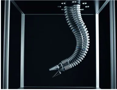
Fig. 1. Festo’s Bionic Handling Assistant is a continuum manipulator with three sections and a gripper. This continuum manipulator changes its pose by deflating or inflating its nine parallel and serial arranged bellows. (Source: Festo AG).
However, due to the complexity, all these mechanical models were considered in static equilibrium only.
Dynamic models for continuum manipulators or the related hyperredundant manipulators were investigated already in the early stages to find a closed-form description [11], but compared with kinematic models, the progress of dynamic models is still lacking [9].
Only a few are using Cosserat rod models for dynamic sim-ulations of single-section manipulators [12] and manipulators with multiple sections [13], but the resulting partial differential equations are not suitable for fast online simulations or con-troller design but rather for general simulations of soft robotics under friction and external loads.
A close approximation of geometrically exact solutions of hy-perflexible and hyperredundant manipulators can be achieved by discretizing continuous models resulting multiple discs or slices. Using mass and stiffness matrices of the slices, the dynamic equations of the manipulator are obtained by integrating over multiple discs. Early works cover the spatial dynamic modeling of single-section manipulators [14] and the planar modeling of multisectional manipulators [15], [16]. For manipulators with many modules, also recursive algorithms for spatial modeling [17] were developed. More recent works obtain the dynamic models of slice approximated manipulators using modal trans-formations and Lagrangian [18] or the principle of virtual work [19]. Although these models might be well suited for simula-tions, they are not applicable to model-based control design.
Lumped models are common for rigid-link robots as they provide rather simple but powerful models suitable for fast simulations and model-based control. However, lumped mass approaches for continuum robots are still hard to find. On the
TABLE I NOMENCLATURE
Symbol Variable name
n number of sections
qi k actuator state of sectioniand bellowsk qi actuator states of sectioni
qj actuator statej
ki configuration state of sectioni φi orientation of sectioni(config. state) κi curvature of sectioni(config. state) ℓi elongation of sectioni(config. state) ψi bending angle of sectioni
jHi homogen. transf. matrix of frameiin ref. framej jRi rotation matrix of frameiin reference framej r position (rin homogeneous representation) g gravity vector
F force (Fin homogeneous representation) Mi ,bend bending momentum of sectioni
mi mass of sectioni
JSi moment of inertia of massmi ωi rotational velocity of massmi T kinetic energy
U potential Q generalized force
M mass matrix of dynamic equation C Coriolis matrix of dynamic equation N force vector of dynamic equation τ actuation force vector of dynamic equation
Index Subscript and superscript description
w world
ih head of sectioni ib base of sectioni Si center of mass of sectioni
Bik center of bellows area of sectioniand bellowsk e active (effective) force
a actuation force p passive force
⋆ general placeholder for similar items
one hand, this might be caused by the idea that only continuum models with distributed parameters instead of concentrated pa-rameters resulting in partial differential equations can describe the dynamic complexity of continuum manipulators. On the other hand, most continuum manipulators are not operated close to dynamic boundaries and thus require only kinematic and static mechanical models. However, a few lumped manipulator mod-els for continuum manipulators were developed so far, most of them in the last years.
Lumped approximations for hyperredundant octopus-like manipulators were developed, e.g., to describe the planar motion of an arm by using decoupled actuator models with a diagonal mass matrix resulting in a decoupled differential equation sys-tem obtained by Lagrange formalism [20]. Another algorithm that describes the spatial net motion of a platform with multi-ple arms was derived by recursively computing reaction forces of actuator segments of multiple arms taking into account the dynamics of the adjacent actuators [21]–[23]. Although forces are exchanged, the dynamic actuator models itself are still de-coupled. A planar model for a tendon-driven manipulator was obtained by defining a high number of point masses. The large but sparse stiffness and mass matrices combined with a Rayleigh damping approach could be used for a modal decomposition and modal control [24].
Even less approaches for bellows or muscle-driven continuum manipulators exist. For a single section, a planar model with three masses along the backbone and spring–damper–actuator systems along the actuators was presented using the Euler– Lagrange formalism [25]. However, no dynamic results were provided, and the static simulations were not convincing.
However, the advantages of lumped manipulator models still remain: They are computationally cheap and the methods al-ready developed for flexible multibody systems [26] and rigid-link manipulators [1] can be easily transferred and applied to other lumped models, like inverse dynamics control. Further-more, the control strategy of bellows actuated manipulators that are limited by slow dynamics on the one hand and undesired interaction of the actuators during faster motions on the other hand could be improved using inverse dynamics control.
Hence, in this paper, an explicit lumped dynamic manipula-tor model is presented that provides a useful analytical approx-imation and considers dynamic couplings of parallel and serial actuators using the Euler–Lagrange formalism. The presented model is applicable to continuum manipulators with intrinsic actuators that can be described with kinematics based on homo-geneous transformations like constant curvature kinematics [3], variable curvature [27], or piecewise constant curvature [28] kinematics. Compared with a previous published conference paper [29], also rotational energies are considered now and an outline toward identification of parameters is provided as well.
In order to derive the model, for each section of a multi-sectional continuum manipulator, lumped point masses were chosen. Based on a mass–spring–damper system of a single bellows [30], a lumped section model with spring–damper rep-resentation for each actuator is developed. Using the kinematic model, local forces are transformed into the world reference frame, such that an Euler–Lagrange formalism can be used [1]. Then, the theoretical model is applied to Festo’s Bionic Hand-ling Assistant [31], a bellows-actuated continuum manipulator with three sections (see Fig. 1).
After introducing the kinematic model of the multisectional constant curvature manipulator in Section II, the dynamic model is derived in Section III: First, the general model is presented; then, the generalized forces, the potential, and the kinetic en-ergy are derived. Furthermore, the analytical derivatives of the homogeneous transformations of the kinematic model need to be computed before the resulting dynamic model with its prop-erties can be presented. In Section IV, the dynamic parameters are identified on the example manipulator before the model is reduced in Section V. After an experimental validation of the model in Section VI, a final conclusion is drawn in Section VII.
II. KINEMATICMODEL
Fig. 2. (a) Actuator statesqcan be measured and controlled, while (b) con-figuration stateskdescribe the shape of the manipulator.
First, the different spaces are introduced before the transfor-mation of the forward kinematics is explained.
A. Kinematic Coordinate Frames
In actuator space, the actuator states
q=q11 q12 . . . qn3 T (1a)
=q1 q2 . . . q{3n}T (1b)
ofnsections representing the lengthl of each bellows can be directly measured and controlled (see Fig. 2a). Two indexing methods allow a bellows- and section-wise notation (1a) of the actuator state qik with section index i∈ {1, . . . , n} and
bellows indexk∈ {1,2,3}and a global actuator-wise notation (1b) of all vector elements qj with global actuator indexj∈
{1, . . . ,3n}.
In configuration space, the configuration stateskcharacterize an actuator-independent model of the manipulator by describ-ing its general shape. These configuration states are provided by the kinematic model. A well-suited kinematic model for continuum manipulators with multiple sections is the constant curvature approach [2], [3] that defines the configuration states (see Fig. 2b) as the section’s backbone lengthℓ, its curvatureκ, and the orientationφof the deformation for each sectioniby
ki=φi κi ℓiT. (2)
For highly conical sections, the model can also be extended to a piecewise constant curvature approach [28]. The curvatureκi
is reciprocal to the section’s bending radius, while the product of backbone length and curvature define the bending angleψi
ψi=κiℓi. (3)
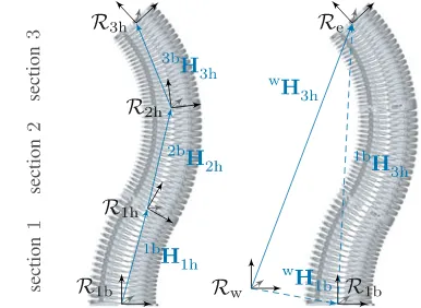
Industrial manipulators are programmed in the end effector’s task frame. These task frames often use Cartesian coordinates as they are very intuitive for humans. Therefore, Cartesian co-ordinate frames Rfor the end effector Re, for the head Rih
and baseRib of the manipulator’s serially linked sections, and
a world reference frame Rw are introduced (see Fig. 3). As
the manipulator cannot twist itself, the task space coordinates
Fig. 3. Serial combination of local task space reference frame defined at each section’s head result in a Cartesian task space representation of a continuum manipulator’s end effector in a world reference frame.
Fig. 4. Kinematic spaces and their corresponding transformations.
consist of three position coordinates and two orientation angles
x=x y z ϕx ϕyT (4)
which can also be expressed by a homogeneous transforma-tion matrix H including a rotation matrixRand a translation vectoro
jH i=
j
Ri joi
01×3 1
∈ R4×4 (5)
that describes the relative pose between two Cartesian coordi-nate framesiandjand allows a derivation of any task coordinate combination, e.g., position only or complete pose.
B. Kinematic Transformations
After defining the coordinate frames, the mappings between these frames need to be determined (see Fig. 4): a specific map-pingfspecificthat calculates configuration stateskin response to
the according actuator statesq and a general mappingfgeneral
that transforms configuration states into task states.
The specific mappingfspecificdescribes the relation between
actuator states and the configuration states for each sectioni. Using the constant curvature approach [3], the configuration states (2) are obtained from actuator states (1) by
fspecific: ki=ki(qi1, qi2, qi3) =ki(qi). (6)
in the transformation equations1[28]
If all three actuators have the same length such that the sec-tion is not bent but straight, the curvature κi is zero, and the
orientationφiis not defined.
The general mapping
fgeneral,loc: ibHih=ibHih(ki) (8)
between the base (index b) and the head element (index h) of a single sectioniis based on the homogeneous transformation (5) and defines the pose of each section’s head. As the configu-ration states are manipulator-independent, the definition of the general transformation is valid for all continuum manipulators with constant curvature and is obtained by
ibH
using the abbreviations
cφ = cosφi, sφ = sinφi, (10a)
cκℓ = cosκiℓi, sκℓ = sinκiℓi. (10b)
If the curvatureκiis zero and the section’s orientationφiis not
defined, (9) becomes
ibH
implying an upright section that is only characterized by its lengthℓi.
The general mapping fgeneral of the tool at the head of the
upper sectioni=nin relation to a world reference frame with
fgeneral,glob: wHih=wHih(k) (12)
is obtained by sequentially stacking the serial sections on top of each other. In this case, the section’s base coordinates are identical with the head coordinates of the section below such that
{i−1}hH
ib =I4 (13)
withIn being the identity matrix of dimensionn. Therefore,
the transformation of a vector in head coordinates of a sectioni
1arctan2is defined s.t.φ= arctan2(sinφ,cosφ)withφ
∈(−π, π].
into the reference coordinate system Rw (12) is obtained by
calculating the product
wH
of all local sectional transformations (9) and the constant initial transformationwH1b(see Fig. 3).
III. DYNAMICMODEL
In order to derive a dynamic model of a continuum manip-ulator with multiple sections that can be used for model-based control and that includes all main characteristics like couplings between the bellows and is still computationally efficient, the distributed mass needs to be discretized. The dynamic model for discrete masses is derived using the Euler–Lagrange equations
d
for the general coordinates qj with the kinetic energy T, the
velocity-independent potentialU, and the corresponding gen-eralized forcesQj. Having n discrete masses mi, their total
kinetic energy
is the sum of their translational energies depending on the linear velocity of each masswr˙
Si and the rotational kinetic energies
depending on the rotation rate ωi. The potential U includes
gravitational potentials and rotational spring potentials due to bending. Without loss of generality, translational spring forces due to extension are covered in the generalized forces
Qj =
that consist of the projection of nf active forces wFe at the
positionwrexcluding potential forces considered inU.
A. General Model Derivation
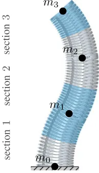
The discrete masses representing the distributed mass and the moments of inertia have to be chosen. Therefore, it is assumed that
r
each sectionihas one concentrated massmilocated at a
locally fixed positionrSi in the section’s head reference
frame (see Fig. 5), and
r
the moments of inertiaihJSi of the discrete masses remain
constant in the local coordinate frame and are approxi-mated as a hollow cylinder.2
Based on these assumptions, the general idea of the model derivation is presented next.
As the manipulator consists of multiple sections, a modular section model is derived first that can be serially coupled later.
Fig. 5. Approximation of distributed masses as point masses located at each section’s head. The top most point mass also includes possible gripper and load masses;m0is fixed.
Fig. 6. Section model with one concentrated mass and three bellows repre-sented by a spring–damper–actuator system (note: 2ndactuator in background).
Therefore, a push–pull actuator–spring–damper model of a sin-gle bellows [30] that characterizes only the longitudinal motion is extended to a section model containing three parallel bel-lows: each section consists of three mass-free bellows modeled as push–pull actuator–spring–damper systems and a combined point mass at the section’s head (see Fig. 6). The gravity forceFg
applies at the center of mass of theithsectionr
Sithat has a fixed
relative position within the section’s head
ih
rSi=const. (18a)
ih
rBik=const. (18b)
as well as the relative positions of the bellow’s contact points rBik. Using the homogeneous transformation (14), position
vectors and forces3are transformed wr
i⋆ =wHihihri⋆ (19)
from the local head coordinate systemRih of the sectionito
the global reference system Rw. The partial derivatives and 3If position vectors are multiplied with a homogeneous transformation, they are extended to[rT1]T, while force vectors are extended to[FT0].T
time derivatives of position vectors that are fixed in the head coordinate system (18) are derived to
∂wr i⋆
∂qik
= ∂
w
Hihihri⋆
∂qik
= ∂
wH ih
∂qik ih
ri⋆+wHih
∂ihr i⋆
∂qik
=0
(20)
and
w˙
ri⋆ =ddt
wH ihihri⋆
=wH˙
ihihri⋆+wHihihr˙i⋆
=0
(21)
and hence only depend on the corresponding derivative of the actuator-dependent homogeneous transformation matrix.
Similarly, rotation rates also depend on homogeneous trans-formation matrices and its derivatives. Using the linear operator Γ{⋆}applied to⋆∈R3×3
Γ{⋆}= diag
⎛
⎝ ⎡
⎣
0 0 1
1 0 0
0 1 0
⎤
⎦⋆ ⎡
⎣
0 0 1
1 0 0
0 1 0
⎤
⎦ ⎞
⎠ (22)
with the properties
∂Γ{⋆}
∂q = Γ
∂ ⋆ ∂q
(23a)
dΓ{⋆} dt = Γ
d⋆ dt
(23b)
and the corresponding homogeneous transformations (5), the rotation ratewωof the massican be derived [32] by
w
ωi= Γ
wR˙ ihwRihT
. (24)
B. Generalized Forces
For the purpose of better interpretation, bellows forces are divided in actuation forces FBik,a (index a) and passive
forcesFBik,p(index p)
FBik,a=FBik,act(pik) =AP·(pik−pamb) (25)
FBik,p=FBik,spr(qik) +FBik,dmp( ˙qik). (26)
The actuation forces result from the pressure difference inside the bellows and the ambient pressure working against the termi-nal surfacesAP. The passive forces are the sum of the
length-dependent longitudinal spring force and the velocity-length-dependent damping force.
With the bellows being always orthogonal to the head and base frame, the forcesFBik ,⋆ transmitted by the bellows apply
orthogonally to head and base atrBik. Therefore, the forces in
the local head and base coordinate frame have only entries in the(z)-direction. By serially stacking multiple sections on top of each other, the actuation and passive net forcesFe,Bik,aand
Fe,Bik,p
ihF
e,Bik,⋆ = ⎧ ⎨
⎩
0 0 FBik,⋆−FB{i+1}k,⋆ 0T i < n
0 0 FBik,⋆ 0T i=n
(27)
External forces in general can apply at every point, but in order to keep the equations as simple as possible, only external forcesFSiapplying at the centers of massrSiare considered in
the following, knowing that extending the resulting equations is easy to perform.
The generalized forcesQj (17) depend on active forces.
Ac-tive forceswFe(index e) are both the external forceswFe,Si w
Fe,Si=wHihihFSi,ext (28)
that apply at the center of mass and are zero if no external contact forces apply and the active forces of the bellowswF
e,Bik w
Fe,Bik =wFe,Bik,a+wFe,Bik,p (29)
consisting of actuation forces and passive forces with the actu-ation forces resulting from the pressure forces of the bellows (25), (27) and the passive forces from the dynamic spring and damper forces
recalling that the active bellows forceswF
e,Bik,⋆are the resulting
forces of a section pair (27) if the section is not the final section. A generalized force (17)
Qik =
for its corresponding actuator stateqikcan be written as a sum
of all projected (20) generalized forces including bellows forces (29) and forces applying at the center of mass (28). Note that gravitation and rotational spring forces due to bending are not included in the generalized forces but in the potentialU.
C. Potential
The potentialUi
Ui=−miwgTwrSi+Mi,bend(ψi, φi) (33)
of a sectioniincludes the gravitational potential of its massmi
located atwrSiand rotational spring momentumMi,bend
depend-ing on the section’s benddepend-ing angleψi (3) and the bending
ori-entationφi. This momentum is introduced, as the longitudinal
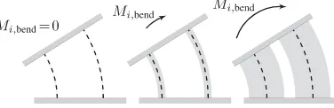
spring force of a bellows (26) derived from the single bellows model only covers the stiffness of its backbone against elonga-tion, but not its width-depending stiffness against lateral applied forces. The resulting net momentum of three parallel bellows (see Fig. 7) disturbing each other’s longitudinal stiffness is taken into account by the rotational spring momentumMi,bend. This
momentum also stabilizes a section to stand straight with zero curvature if no external forces apply.
The partial derivatives of the section’s potential are
∂Ui
Fig. 7. Introduced bending stiffnessMi,bendof sectioniconsiders the lateral stiffness due to the nonzero width of the bellows that forces single bellows to stand straight if no external forces are applied.
The sum of allnsections’ potentials derived by the generalized coordinateqik
∂U
describes the influence of the global potential on the generalized coordinate that is used for Euler–Lagrange equation (15).
D. Kinetic Energy
Using the homogeneous derivative (21) to describe the veloc-ities ofnpoint masses, the kinetic energy (16) with respect to the global reference systemRwis
T =Ttrans+Trot (36)
and the moment of inertia expressed in world coordinates
w
JSξ =wRξhξhJSξwRTξh. (39)
To apply the Euler–Lagrange equations (15), the partial deriva-tives of (36) with respect to all generalized coordinatesqik are
needed. Using the chain rule and the identity4
∂H
∂qj
=∂H˙ ∂q˙j
, (40)
the derivatives of the translational kinetic energy (37) for con-stant massesmiare
∂Ttrans
The derivatives of the homogeneous transformations H used in (41)–(43) are presented in Appendix B. Similarly, the derivatives of the rotation matrixRcan be implemented, as the identity of
∂R
∂q =
∂R˙
∂q˙ (44)
follows (40). To compute the derivatives of the rotational kinetic energy (38) similar to (41)–(43), the properties of the linear operatorΓ(23) are used, such that the derivatives ofTrot
for constant inertiaξhJSξ are
∂Trot
using the abbreviationRforwR
ξhand its derivatives.
E. Resulting Dynamic Model
By inserting the generalized forces (32) for all generalized co-ordinatesqj and the derivatives of potential (35) and the kinetic
energy (41), (43), (45), (47) into the Euler–Lagrange equation (15), 3n coupled second-order differential equations are ob-tained. By resorting, the differential equations can be written in matrix form as
M(q) ¨q+C(q,q˙) ˙q+N(q,q˙) =τ(p), (48)
in which the active, controllable forceswF
Bik,a are part of the
inhomogeneous input force vectorτ(p)of the differential equa-tion. The resulting mass matrixM ∈R3n×3nand the matrix of Coriolis and centrifugal gainsC ∈R3n×3n are defined by the entry-wise formulas matrices and using the abbreviationHforwHξhand its deriva-tives (RforwRξh respectively). The start index of the sums is defined by
s=section of(max(r, c)). (51)
The last three rows of (50) result from nonconstantwJ
Sξ due to
the rotation of constantξhJSξ in the world reference frame (39).
The homogeneous force vectorN ∈R3n
N(r) =
contains stiffness and damping properties, as well as external and gravitational influences, while the pressure-dependent in-homogeneous force vectorτ(p)∈R3n is defined as
with forces in the global (53a) or local (53b) reference frame (19). As the pressures of the bellows are the inputs of the me-chanical model but their progressions cannot be chosen arbitrar-ily, dynamic models for the pneumatic behavior of the individual bellows are necessary as well. The pneumatic model of a bel-lows [30] based on models of pneumatic cylinders [33]–[35] is taken from existing models.
If the model is extended by adding additional external forces, these additional forces need to be separated into passive forces assigned toN, and actuated forces assigned toτ, although the latter should be rather uncommon.
IV. MODELIDENTIFICATION
With the structural model derived (48)–(53), it can be pro-grammed efficiently, but in order to run simulations, parameters need to be identified. All kinematic parameters like the distance of the bellows’ center to the section’s backbonerBi(7b), (18b)
or the sizes of the terminal surfacesAPof the bellows (25) can be
taken from the CAD model or have to be identified beforehand in order to obtain the kinematic model. The position ihrSi of
each section’s mass point in its local head frame (18a) is placed at the center
ih
rSi= [0,0,0,1]T (54)
of the head’s profile. The remaining dynamic parameters that have to be identified are
r
the longitudinal stiffness or spring forceFBik,spr(qik)of
the bellows depending on its elongation,
r
the longitudinal damping forceFBik,dmp( ˙qik)of the
bel-lows depending on its velocity,
r
each section’s bending momentumMi,bend(ψi)depending
on the bending angle of the section,
r
the nominal massmiof each section, and
r
the corresponding constant moments of inertial ihJSi of
each mass.
In the following, these functions and constant parameters are identified on the Bionic Handling Assistant with appropriate experiments and measurements.
A. Identification of the Nominal Section Mass
The point massmi of a section is an approximation of the
real mass distributed over the whole section. A sufficient ap-proximation of the section’s mass can be obtained by weighing the individual sections before assembling. Other masses being moved like tubes and wire cables are below1 %of the mass of a section’s polyamide structure and therefore neglected.
B. Identification of Inertia
The inertia of each section can obtained by a static model from CAD or approximated by a solid cylinder of average section heightℓiavgand radiusrBi+rbias sum of bellow’s backbone
distance plus bellow’s radius. The local inertia tensor results in
ihJ Si =
⎡
⎢ ⎣
ihJ
Si,x 0 0
0 ihJ
Si,y 0
0 0 ihJ
Si,z ⎤
⎥
⎦ (55)
with the moments of inertia defined as
ihJ
Si,x= 14mi(rBi+rbi)2+121 miℓ2iavg, (56a) ihJ
Si,y = 14mi(rBi+rbi)2+121 miℓ2iavg, (56b) ihJ
Si,z= 12mi(rBi+rbi)2. (56c)
Fig. 8. Identification of the nonlinear stiffness behavior by measuring steady-state pressures for several elongations.
However, an approximation of the maximum moment of inertia can be obtained by assuming a hollow cylinder with maximal section lengthℓim ax and radiusrBi+rbi
ihJ
Si,xm ax = 12mi(rBi+rbi)2+121 miℓ2im ax (57a)
ihJ
Si,ym ax = 12mi(rBi+rbi)2+121 miℓ2im ax (57b)
ihJ
Si,zm ax = mi(rBi+rbi)2 (57c)
that is used for the calculation of a maximum bound of rotational energies.
These constant moments of inertia in the local frameRihcan
be transformed intoRwusing (39) and the rotation matrixwRih
of the corresponding homogeneous transformation (5). The im-plementation of variable local inertia matricesihJSi depending
on the configuration states (section length, curvature, and ori-entation) is not worth the effort due to its small influence at possible motions.
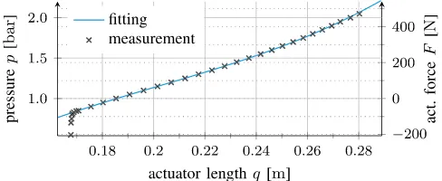
C. Identification of Longitudinal Stiffness
The longitudinal stiffness of the bellows is represented by the bellows’ spring forceFBik,spr(qik), which is a nonlinear function
depending on the length of each actuator (26). As a steady-state force, it can be identified by elongating all bellows of each sec-tion evenly such that the secsec-tions curvature stays zero (7). The spring forces are obtained by calculating actuation forces from measured steady-state pressures (25) and subtracting gravita-tional influences (see Fig. 8).
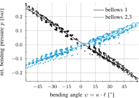
D. Identification of Bending Stiffness
The bending stiffness of a section represented by the section’s bending momentumMi,bend depends on the bending angleψi
Fig. 9. Linear fitting of the relative bending pressures versus bending angle of bellows 1 working against bellows 2 and 3. Negative curvature indicates bending in the other directionφ=π.
Fig. 10. Lateral swing triggered by contact loss of an external force to iden-tify the manipulator’s damping properties. Oscillations are visible on lateral deflection of the three sectionsxand a selection of actuator lengthsq.
E. Identification of Longitudinal Damping
Due to small velocities, the damping forcesFBik,dmp( ˙qik)of
each bellows (26) have a small impact on dynamics if the ma-nipulator is driven only by actuator force. However, on swings and oscillations triggered by jumps in external forces, e.g., a loss of contact (see Fig. 10), damping forces characterize the frequency and the decay of the oscillation. Using a least-squares fit, linear damping parameters can be identified from manipula-tor oscillations (see Fig. 10).
V. MODELREDUCTION
When running dynamic simulations, a detailed model is de-sired. However, small errors are acceptable if the model is used for model-based control such that small errors can be com-pensated by feedback control and the computation time can be reduced significantly—e.g., for inverse dynamics control and model-based decoupling of the actuators using feedback-linearization [36].
In the following, two model reduction approaches are pre-sented: First, rotational kinetic energies are neglected for the computation of the dynamic matricesM andC. Second, the influence of the Coriolis matrixC on the dynamic model (48) is investigated and how the model changes if Coriolis forces are neglected.
Fig. 11. Comparison of the measured translational energy and upper bounded rotational energy (57) of a lateral swing (see Fig. 10) with maximal rotation.
A. Neglecting Rotational Kinetic Energies
Rotational kinetic energiesTrot(16) are high on classic
indus-trial robots with rigid arms and rotational joints as all motions are based on rotations only, especially due to the decreasing iner-tia of outer arms. Continuum manipulators do not have this kind of rotational joint. Rotations are comparably slow and can be imposed only by contrary extending and contracting bellows of a single section. Furthermore, the main motions of the imposed section mass and the attached sections will be of translational manner as, for example, a bending of the first section results in a small rotation of the upper sections but also in a large translation of the upper sections due to their leverage factor. Using a maximum approximation of each section’s inertia (57), the rotational kinetic energy of a lateral swing (see Fig. 10) with maximal rotational velocities is significantly lower than the translational kinetic energy (see Fig. 11). Compared with this worst-case scenario, other motions generated by actuation force instead of external contact loss contain even less rotational kinetic energies.
Therefore, rotational kinetic energies can be neglected [29] for some purposes, especially for model-based control where computation time is important and small errors can be compen-sated by feedback control. This leads to a large simplification of the dynamic mass matrixM and the Coriolis matrixCsuch that the main dynamics are reduced to
M(r,c)=
n
ξ=s
mξ $∂wH
ξh
∂qc ξhr
Sξ %T∂wH
ξh
∂qr ξhr
Sξ (58)
C(r,c)=
n
ξ=s
mξ "
∂wH˙ ξh
∂qc ξh
rSξ #T
∂wH
ξh
∂qr ξh
rSξ (59)
instead of (49) and (50). The homogeneous force vectorNand the pressure-dependent inhomogeneous force vector τ(p) do not depend on kinetic energies and therefore remain the same.
B. Neglecting Coriolis and Centrifugal Forces
The computation of the Coriolis and centrifugal gain matrix C in the dynamic equation (48) is computational very heavy even if rotational kinetic energies are neglected. The high com-putational burden is caused by the dependence on the partial derivative∂hwH˙ξ/∂qj that is used only inC(50), (59) but takes
TABLE II
SELECTEDPARAMETERS OF THEEXAMPLEMANIPULATOR
Symbol Value
Mass per section [kg] 1.25 Pressure range (abs.) [105 Pa] 0.5. . .2.0 Pressure force [N] -200. . .500 Bellows length range [m] 0.17. . .0.29 Bellows volume [10−3 m3] 0.23. . .0.57
the Coriolis matrix
C(r,c) =
n
ξ=s
mξ
"
∂wH˙ ξh
∂qc ξhr
Sξ #T
∂wH
ξh
∂qr ξhr
Sξ ≈0 (60)
loses influence. If computation time is to be reduced, the Coriolis matrix of the dynamic model can be neglected
M(q) ¨q+N(q,q˙) =τ(p) (61)
depending on the required accuracy of the model.
Comparisons between measurements and simulation for both model reduction approaches are shown in the experimental val-idation next.
VI. EXPERIMENTALVALIDATION
In order to test and verify the presented model and its ap-proximations, measurements on the Bionic Handling Assistant were compared with open loop simulations of the model using the parameters from Table II.
Measurements are recorded using a DSpace 1007 PPC with 1 ms sampling time. Reference measurements were obtained from a pressure controlled manipulator. Note that negative pressures up to approximately −0.3bar can be applied to the bellows using vacuum, in order to achieve higher curvatures—i.e., if two bellows of a section are pressurized, the third can be artificially held short.
Simulations were implemented in MATLAB/Simulink in-cluding the analytical derivatives of the homogeneous transfor-mations ((66), Appendix B). Singularities in the mathematical formulation of the kinematic model were excluded numerically to distinguish between curvatureκclose to zero (11) instead of (9) using switching boundary ofκ= 1·10−6.
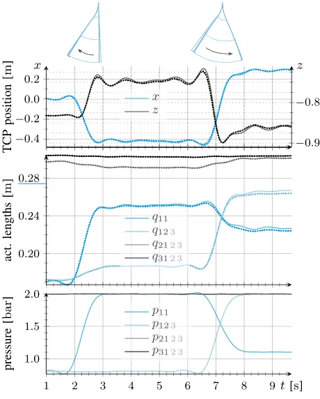
First, experiments with an actuated manipulator were con-ducted. Therefore, some bellows were actuated using a pressure trajectory, while the remaining were held at constant pressure. However, due to the mechanical coupling of the actuators, even the nonactuated bellows change their length. By changing only the pressure of the first bellows in the first section and in a second step the pressures of all bellows in the first section, two tilting motions are created (see Fig. 12). The second and third sections are extended in order to create a larger inertia.
These measurements can be compared with a simulation of the full model (49), (50) and a reduced model neglecting both rotational kinetic energies and Coriolis forces (58), (61). During pressure-driven motions, both models are good approximations of the measured trajectories. However, static models cannot describe the motions that well (see Fig. 13). A
Fig. 12. Reference measurement data (—–) versus simulated trajectories of a full model (· · · ·) including rotational kinetic energies and Coriolis influences and a reduced model (– – –) without rotational kinetic energies and Coriolis influences.
Fig. 14. Reference measurement data of a lateral swing (—–) versus simu-lated trajectories of a full model (· · · ·) including rotational kinetic energies and Coriolis influences and a reduced model (– – –) without rotational kinetic energies and Coriolis influences.
decoupled actuator model taking into account only translational spring forces against static pressures does not describe dynamic effects, gravity, and bending. A static model
N(q,q˙) =τ(p) (62)
derived from (48) that takes into account also bending and gravity has also large errors during motions. Furthermore, the actuator lengths q cannot be computed explicitly from (62), and computing the solution implicitly takes even longer than the dynamic simulation.
Second, lateral swing motions similar to the damping iden-tification (see Fig. 9) experiment are investigated. Actuated by the loss of an external contact force, the manipulator conducts a damped oscillation although the pressures in the bellows are not controlled (see Fig. 14). These motions cannot be simu-lated with static models, as the steady state does not change as long as the pressure in the bellows does not change. The developed dynamic models however—both full models and re-duced models—can describe the motion quite well (see Fig. 14). The simulated frequency, amplitude, and damping of the tool center point (TCP) matches the reference measurement during the large oscillations at the beginning of the swing. However,
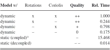
TABLE III
COMPARISON OF THERELATIVECOMPUTATIONTIME
Modelw/ Rotations Coriolis Quality Rel. Time
dynamic x x ++ 1.000
dynamic x – ++ 0.244
dynamic – x + 0.798
dynamic – – 0 0.175
static (coupled)a – 15.468
static (decoupled) – – 0.014
aHigh computational effort due to an implicit nonlinear model.
simulation errors, especially in the actuator domain, exist due to limits of the lumped mass approximation of the manipulator. All further approximations made in the model reduction section— neglecting rotational kinetic energies and Coriolis forces—lead to very small changes in the simulation results, while the com-putation time decreases by about80 %. A comparison of relative computation times with respect to the full dynamic model (48) is presented in Table III. It provides the computational effort of the methods independently of simulation step size, computational power, and simulation time.
VII. CONCLUSION
In this paper, a new approach for a dynamic model of bellows-actuated spatial continuum manipulators has been presented that includes couplings and interconnections between the parallel and serial arranged bellows. Doing this, each section is modeled as a single lumped mass point actuated by three parallel spring– damper systems. Using the constant curvature kinematic model, forces between the sections are transformed into a common world reference system such that the Euler–Lagrange equations for each actuator can be computed. With analytic derivatives of kinematics, the dynamic manipulator model can be easily implemented. After a parameter identification on the example manipulator, experiments show that the new model incorporates the interconnections between the bellows and that it describes the real manipulator behavior well. In order to reduce compu-tation time, the complexity of the model can be reduced even further, if the desired accuracy is not as important—e.g., for inverse dynamics control and model-based decoupling of the actuators using feedback linearization.
APPENDIXA
PROVING THEIDENTITY OFHOMOGENEOUSDERIVATIVES
The identity of∂∂ qjH = ∂H˙
∂qj˙ as stated in (40) is a common result from classical mechanics. However, due to its importance for the derivation of the dynamical model, a short proof will be presented here.
Proof: The identity of (40) can be validated by using the property
∂r
∂q =
∂r˙
∂q˙ (63)
derived from the principle of virtual work [37] that is valid ifr
ofr(19) andr˙(21) are
Withihri⋆ being constant (18) and its partial derivatives being
zero, the assumption (40) follows the property (63).
APPENDIXB
DERIVATIVES OFCONCATENATED
HOMOGENEOUSTRANSFORMATIONS
The derivatives of the homogeneous transformation of a sin-gle sectionibHih(k(q))can be obtained by applying the chain rule, using the general mapping fgeneral (12) and the specific
mappingfspecific(6) of the constant curvature approach. As the
homogeneous transformation of a single sectionˆιbHˆιhonly de-pends on the actuator statesqikof this section, the derivative
∂ˆιbH
is zero with respect to actuator states of other sections. Hence, the derivative of a global homogeneous transformationwHˆιh
∂wH
is independent of sections i and actuators qik that are above
sectionˆι. Similar to (66), also the second partial derivatives of a section
with respect to actuator states of other sections are zero. Fol-lowing (67) and defining without loss of generalityα≤i, the second partial derivative
∂2 wH of a homogeneous transformation in the world reference frame can be derived.
The resulting time derivative of the time-invariant transfor-mationwHˆιh
only depends on partial derivatives and the corresponding ac-tuator velocities, similar to the partial derivative of the time derivative
that equals the time derivative of the partial derivative
d
The second time derivative of homogeneous transformations in the world reference framewH¨ˆιh
used in (43) is obtained by using (40) and can be computed with partial derivatives of first (67) and second order (69) and the time derivatives of the actuator statesq.
Using the chain rule, the derivatives of the section’s specific mapping (7) as well as the partial derivatives of the sections general mapping (9) used in (66) and (68) can be computed analytically [28] and then inserted into the formulas of the global derivatives. Similarly, all derivatives of rotation matriceswRih can be computed, too.
REFERENCES
[1] B. Siciliano and O. Khatib, Eds.,Handbook of Robotics. Heidelberg, Germany: Springer, 2008.
[2] B. Jones and I. Walker, “Kinematics for multisection continuum robots,”
IEEE Trans. Robot., vol. 22, no. 1, pp. 43–55, Feb. 2006.
[4] D. B. Camarillo, C. F. Milne, C. R. Carlson, M. R. Zinn, and J. K. Salisbury, “Mechanics modeling of tendon-driven continuum manipulators,”IEEE Trans. Robot., vol. 24, no. 6, pp. 1262–1273, Dec. 2008.
[5] R. J. Webster, J. M. Romano, and N. J. Cowan, “Mechanics of precurved-tube continuum robots,”IEEE Trans. Robot., vol. 25, no. 1, pp. 67–78, Feb. 2009.
[6] D. Trivedi, A. Lotfi, and C. Rahn, “Geometrically exact models for soft robotic manipulators,”IEEE Trans. Robot., vol. 24, no. 4, pp. 773–780, Aug. 2008.
[7] F. Renda, M. Cianchetti, M. Giorelli, A. Arienti, and C. Laschi, “A 3D steady-state model of a tendon-driven continuum soft manipulator inspired by the octopus arm,”Bioinspiration Biomimetics, vol. 7, no. 025006, pp. 1–12, 2012.
[8] K. Xu and N. Simaan, “Analytic formulation for kinematics, statics, and shape restoration of multibackbone continuum robots via elliptic inte-grals,”J. Mechanisms Robot., vol. 2, no. 1, pp. 1–13, Feb. 2010. [9] I. Walker, “Continuous backbone continuum robot manipulators,”ISRN
Robot., vol. 2013, p. 726506, 2013.
[10] J. Jung, R. S. Penning, N. J. Ferrier, and M. R. Zinn, “A modeling approach for continuum robotic manipulators: Effects of nonlinear internal device friction,” inProc. IEEE/RSJ Int. Conf. Intell. Robots Syst., Sep. 2011, pp. 5139–5146.
[11] G. Chirikjian, “Hyper-redundant manipulator dynamics: A continuum ap-proximation,”Adv. Robot., vol. 9, no. 3, pp. 217–243, Jan. 1995. [12] C. Rucker and R. Webster, “Statics and dynamics of continuum robots
with general tendon routing and external loading,”IEEE Trans. Robot., vol. 27, no. 6, pp. 1033–1044, Dec. 2011.
[13] F. Renda, M. Giorelli, M. Calisti, M. Cianchetti, and C. Laschi, “Dynamic model of a multibending soft robot arm driven by cables,”IEEE Trans. Robot., vol. 30, no. 5, pp. 1109–1122, Oct. 2014.
[14] H. Mochiyama and T. Suzuki, “Dynamical modeling of a hyper-flexible manipulator,” inProc. 41st SICE Annu. Conf., 2002, pp. 1505–1510. [15] E. Tatlicioglu, I. D. Walker, and D. Dawson, “Dynamic modelling for
planar extensible continuum robot manipulators,” inProc. 2007 IEEE Int. Conf. Robot. Autom., 2007, pp. 1357–1362.
[16] E. Tatlicioglu, I. D. Walker, and D. Dawson, “New dynamic models for pla-nar and extensible continuum and robot manipulators,” inProc. IEEE/RSJ Int. Conf. Intell. Robots Syst., Oct. 2007, pp. 1485–1490.
[17] G. Gallot, O. Ibrahim, and W. Khalil, “Dynamic modeling and simulation of a 3-D hybrid structure eel-like robot,” inProc. IEEE Int. Conf. Robot. Autom., Apr. 2007, pp. 1486–1491.
[18] I. Godage, D. Branson, E. Guglielmino, G. Medrano-Cerda, and D. Cald-well, “Dynamics for biomimetic continuum arms: A modal approach,” in
Proc. IEEE Int. Conf. Robot. Biomimetics, 2011, pp. 104–109.
[19] W. Rone and P. Ben-Tzvi, “Continuum robot dynamics utilizing the prin-ciple of virtual power,”IEEE Trans. Robot., vol. 30, no. 1, pp. 275–287, Feb. 2014.
[20] Y. Yekutieli, R. Sagiv-Zohar, R. Aharonov, Y. Engel, B. Hochner, and T. Flash, “Dynamic model of the octopus arm. I. biomechanics of the octopus reaching movement,” J. Neurophysiol., vol. 94, no. 2, pp. 1443–1458, May 2005.
[21] R. Kang, D. T. Branson, E. Guglielmino, and D. G. Caldwell, “Dynamic modeling and control of an octopus inspired multiple continuum arm robot,”Comput. Math. Appl., vol. 64, no. 5, pp. 1004–1016, Sep. 2012. [22] T. Zheng, D. T. Branson, R. Kang, M. Cianchetti, E. Guglielmino,
M. Follador, G. A. Medrano-Cerda, I. S. Godage, and D. G. Caldwell, “Dynamic continuum arm model for use with underwater robotic ma-nipulators inspired by octopus vulgaris,” inProc. IEEE Int. Conf. Robot. Autom., pp. 5289–5294, May 2012.
[23] T. Zheng, D. T. Branson, E. Guglielmino, R. Kang, G. A. M. Cerda, M. Cianchetti, M. Follador, I. S. Godage, and D. G. Caldwell, “Model val-idation of an octopus inspired continuum robotic arm for use in underwater environments,”J. Mech. Robot., vol. 5, no. 2, 2013.
[24] R. S. Penning and M. R. Zinn, “A combined modal-joint space con-trol approach for continuum manipulators,”Adv, Robot., vol. 28, no. 16, pp. 1091–1108, Jul. 2014.
[25] N. Giri and I. Walker, “Three module lumped element model of a contin-uum arm section,” inProc. IEEE/ RSJ Int. Conf. Intell. Robots Syst., Sep. 2011, pp. 4060–4065.
[26] A. Jain and G. Rodriguez, “Recursive flexible multibody system dynamics using spatial operators,”J. Guid. Control Dyn., vol. 15, pp. 1453–1466, Nov. 1992.
[27] T. Mahl, A. Mayer, A. Hildebrandt, and O. Sawodny, “A variable curvature modeling approach for kinematic control of continuum manipulators,” in
Proc. Am. Control Conf., 2013, pp. 4952–4957.
[28] T. Mahl, A. Hildebrandt, and O. Sawodny, “A variable curvature contin-uum kinematics for kinematic control of the Bionic Handling Assistant,”
IEEE Trans. Robot., vol. 30, no. 4, pp. 935–949, Aug. 2014.
[29] V. Falkenhahn, T. Mahl, A. Hildebrandt, R. Neumann, and O. Sawodny, “Dynamic modeling of constant curvature continuum robots using the Euler-Lagrange formalism,” inProc. IEEE/ RSJ Int. Conf. Intell. Robots Syst., 2014, pp. 2428–2433.
[30] V. Falkenhahn, A. Hildebrandt, and O. Sawodny, “Trajectory optimization of pneumatically actuated, redundant continuum manipulators,” inProc. Am. Control Conf., 2014, pp. 4008–4013.
[31] A. Grzesiak, R. Becker, and A. Verl, “The Bionic Handling Assistant: A success story of additive manufacturing,”Assembly Autom., vol. 31, no. 4, pp. 329–333, 2011.
[32] B. Siciliano, L. Sciavicco, L. Villani, and G. Oriolo,Robotics—Modelling, Planning and Control. New York, NY, USA: Springer, 2009.
[33] A. Hildebrandt, O. Sawodny, R. Neumann, and A. Hartmann, “A flatness based design for tracking control of pneumatic muscle actuators,” inProc. 7th Int. Conf. Control Autom. Robot. Vis., vol. 3, 2002, pp. 1156–1161. [34] A. Ilchmann, O. Sawodny, and S. Trenn, “Pneumatic cylinders: Modelling
and feedback force-control,”Int. J. Control, vol. 79, no. 6, pp. 650–661, Jun. 2006.
[35] A. Hildebrandt, R. Neumann, and O. Sawodny, “Optimal system and de-sign of SISO-servopneumatic and positioning drives,”IEEE Trans. Con-trol Syst. Technol., vol. 18, no. 1, pp. 35–44, Jan. 2010.
[36] V. Falkenhahn, A. Hildebrandt, R. Neumann, and O. Sawodny, “Model-based feed-forward position control of constant curvature continuum robots using feedback linearization,” inProc. IEEE Int. Conf. Robot. Autom., 2015, pp. 762–767.
[37] M. Spong, S. Hutchinson, and M. Vidyasagar,Robot Modeling and Con-trol. Hoboken, NJ, USA: Wiley, 2006.
Valentin Falkenhahn received the Dipl.-Ing. de-gree in engineering cybernetics from the University of Stuttgart, Stuttgart, Germany, in 2012, where he is also working toward the Ph.D. degree in a joint project with Festo AG & Co. KG, Esslingen, Ger-many.
He is currently a Research Assistant with the In-stitute for System Dynamics, University of Stuttgart. His current research interests include modeling, iden-tification, and model-based control of pneumatic, electrical, and biomechanical systems and industrial applications of system engineering.
Tobias Mahlreceived the Dipl.-Ing. degree in engi-neering cybernetics from the University of Stuttgart, Stuttgart, Germany, in 2007, and the Ph.D. degree from the University of Stuttgart in 2015.
He is currently a Research Assistant with the In-stitute for System Dynamics, University of Stuttgart. His current research interests include modeling, iden-tification, and control of mechatronic systems and in-dustrial applications of system engineering.
Alexander Hildebrandtreceived the Dipl.-Ing. de-gree in electrical engineering from Ulm University, Ulm, Germany, in 2002, and the Ph.D. degree from the University of Stuttgart, Stuttgart, Germany, in 2009.
R ¨udiger Neumannreceived the Dipl.-Ing. degree in mechanical engineering from the University of Pader-born, PaderPader-born, Germany and University of Notting-ham, NottingNotting-ham, UK, in 1986, and the Ph.D degree from the University of Paderborn and Ulm Univer-sity, Ulm, Germany, in 1995.
Since 1996, he has been an Engineer of automation and control with the Research Department, Festo AG & Co. KG, Esslingen, Germany, where he is cur-rently the Head of the Department for Mechatronic Systems. His research interests include the control of pneumatic and electrical servo drives, as well as control of multiaxes systems and robots.
Oliver Sawodnyreceived the Dipl.-Ing. degree in electrical engineering from the University of Karl-sruhe, KarlKarl-sruhe, Germany, in 1991, and the Ph.D. degree from the Ulm University, Ulm, Germany, in 1996.