Associating Uncertainty With Three-Dimensional
Poses for Use in Estimation Problems
Timothy D. Barfoot
, Member, IEEE
, and Paul T. Furgale
, Member, IEEE
Abstract—In this paper, we provide specific and practical
ap-proaches to associate uncertainty with 4×4 transformation ma-trices, which is a common representation for pose variables in 3-D space. We show constraint-sensitive means of perturbing trans-formation matrices using their associated exponential-map gener-ators and demonstrate these tools on three simple-yet-important estimation problems: 1) propagating uncertainty through a com-pound pose change, 2) fusing multiple measurements of a pose (e.g., for use in pose-graph relaxation), and 3) propagating uncertainty on poses (and landmarks) through a nonlinear camera model. The contribution of the paper is the presentation of the theoretical tools, which can be applied in the analysis of many problems involving 3-D pose and point variables.
Index Terms—Exponential maps, homogeneous points, matrix Lie groups, pose uncertainty, transformation matrices.
I. INTRODUCTION
T
HE main contribution of this paper is to provide simple and practical techniques to associate uncertainty with 4×4 transformation matrices (commonly used to represent pose vari-ables) for use in robotic estimation problems. The challenge in choosing a representation of pose and its associated uncertainty is that representations either have singularities or constraints; this results from the fact that rotation variables are notvectors but rather members of anoncommutative group. The advantage of the technique that we will present is that it is free of singu-larities but avoids the need to enforce constraints when solving optimal estimation problems. This is accomplished by storing the mean as a (singularity-free) 4×4 transformation matrix and using a 6×1 (constraint-sensitive) perturbation of the pose (with an associated 6×6 covariance matrix). As we will see, our approach amounts to getting the best of both worlds as it facilitates rather straightforward implementations of common estimation problems such as bundle adjustment [1].Transformation matrices are by no means new, having risen to popularity through manipulator robotics [2] and computer vision [3]. We will use standard definitions for thespecial orthogonal
Manuscript received August 8, 2013; revised November 17, 2013; accepted December 20, 2013. Date of publication January 28, 2014; date of current ver-sion June 3, 2014. This paper was recommended for publication by Associate Editor R. Eustice and Editor D. Fox upon evaluation of the reviewers’ comments. This work was supported by the Natural Sciences and Engineering Research Council of Canada and the EU FP7 2007–2013 Programme, Challenge 2, Cog-nitive Systems, Interaction, Robotics, under Grant 269916, V-Charge.
T. D. Barfoot is with the Autonomous Space Robotics Lab, University of Toronto, ON M5S 2J7, Canada (e-mail: [email protected]).
P. T. Furgale is with the Autonomous Systems Lab, ETH Zurich, 8092 Zurich, Switzerland (e-mail: [email protected]).
Color versions of one or more of the figures in this paper are available online at http://ieeexplore.ieee.org.
Digital Object Identifier 10.1109/TRO.2014.2298059
groupthat represents rotation
SO(3) :=C∈R3×3 |CCT =1,detC= 1 where1is the identity matrix, and thespecial Euclidean group that represents rotation and translation
SE(3) :=
T=
C r
0T 1
∈R4×4
{C,r} ∈SO(3)×R3
.
(1) Both are examples ofmatrix Lie groups, for which Stillwell [4] provides an accessible introduction. We will avoid rehashing the basics of group theory here but stress that we cannot apply the usual approach of additive uncertainty for such quantities as they are not members of avector space. In other words
x= ¯x+δ (2)
where x∈Rn is a random variable, ¯xis a ‘large,’ noise-free value, andδis a ‘small,’ uncertain perturbation (i.e., zero-mean noise), which does not directly apply to members of SO(3) andSE(3). This paper investigates one means to overcome this problem.
In robotics, it has been well established that estimating un-certain spatial relationships is a fundamentally important prob-lem. For example, the early works of Brooks [5], Smith and Cheeseman [6], Durrant-Whyte [7], and Smithet al.[8] spurred the popular subfield of simultaneous localization and map-ping[9]. Our approach is similar to the work of Chirikjian [10] and [11], who provide a rigorous treatment of representing and propagating uncertainty on Lie groups. It is also related to and extends the ideas presented by Su and Lee [12], [13] and Smith et al.[14]. Finally, in a recent paper, Hertzberget al.[15] take a similar approach to associate uncertainty with general mani-folds, while we provide more details on handlingSE(3) specif-ically. One could view our paper as providing an accessible and specific implementation of a means of associating and ma-nipulating uncertainties forSE(3)[and, thus, collaterally with
SO(3)]. The differences between our approach and the pre-viously published works are subtle but important. Rather than list them here in detail, we will take care to point out specific differences throughout the paper, then summarize them in the conclusion.
We also demonstrate the usefulness of our method on three key problems: 1) propagating uncertainty through a compound-ing of two transformation matrices, 2) fuscompound-ing multiple uncertain measurements of a pose into a single estimate, and 3) propagat-ing pose (and landmark) uncertainty through a nonlinear (stereo) camera model. In our calculations, we will retain as many terms in the noise variables as possible, thereby demonstrating the power of our approach.
This paper is organized as follows. Section II presents the mathematical machinery that we will use throughout the paper. Section III discusses how to compound two poses and their uncertainties, Section IV shows how to fuse multiple estimates of pose together, and Section V shows how to propagate pose and landmark uncertainty through a nonlinear measurement model. A conclusion rounds out the paper.
II. MATHEMATICALPRELIMINARIES
A. Random Variables and Probability Density Functions
In contrast with (2), we will define random variables for
SE(3)according to
T:= exp ξ∧T¯ (3) whereT¯ ∈SE(3)is a ‘large,’ noise-free value, andξ∈R6is a ‘small,’ noisy perturbation. The∧operator1turnsξinto a 4
×4 member of theLie algebrase(3)according to
ξ∧:=
ρ φ
∧
=
φ∧ ρ 0T 0
(4)
whereρ,φ∈R3 are 3×1, and∧also turnsφinto a member of theLie algebraso(3):
φ∧:= ⎡
⎣
φ1
φ2
φ3 ⎤
⎦
∧
= ⎡
⎣
0 −φ3 φ2
φ3 0 −φ1
−φ2 φ1 0
⎤
⎦. (5)
We will use∨as the inverse operation of∧. This perturbation approach ensures thatT∈SE(3)and is sometimes referred to as aninjectionof noise onto the groupSE(3)[20]. Additional notation and a closed-form expression for the matrix exponential in (3) can be found in the Appendix.
In this paper, we will define the small perturbation variable to be zero-mean Gaussianp(ξ) =N(0,Σ), whereΣis a 6×6 covariance matrix. We stress that we are directly defining this probability density function (PDF) in the vectorspace,R6. This choice in turn induces a PDF over SE(3), p(T). To see what this PDF is, we note that by our definition
R6
p(ξ)dξ=
R6
ηexp
−12ξTΣ−1ξ
dξ= 1 (6) whereη= √ 1
(2π)6det(Σ) is the (constant) normalization factor.
To switch variables and write a PDF overT, we must define what we mean by an infinitesimal volume ofSE(3), which is written asdT. Along the lines of Chirikjian [11], we will relate perturbations inξto perturbations inTaccording to
δT:= ln T′T−1∨ (7)
1The∧operator is ‘overloaded’ in the sense that it can be applied to both 6×1 and 3×1 columns [2] [11] [16]. For the 6×1 case,∧is similar to the⊞operator defined by [17] but without the negative sign in front of theρcomponent. For the 3×1 case,φ∧is sometimes written asφ×[18] or[[φ]][19]; sometimes, the∧is written above the symbol, as inφ; however, we shall stick to the originalˆ definition in Murrayet al.[2, pp. 26 and 41], which has it off to the right, since we often apply it to expressions involving multiple variables.
where
T′:= exp (ξ+δξ)∧T¯, T:= exp ξ∧T¯. (8) It can then be shown that
δT=Jδξ (9)
where
J := 1
0
exp ξα dα (10) is referred to as theJacobianforSE(3)[21]; we will discuss this in more detail in the next section. We define theoperator2
to be
ξ=
ρ φ
=
φ∧ ρ∧
0 φ∧
(12)
which is 6×6. We will also useas the inverse operation of , for convenience.
The infinitesimal volume elements can then be related [21] by
dT=|det (J)|dξ. (13) Usingξ= ln TT¯−1∨ and (13) in (6), we may find the PDF overTby a straightforward change of coordinates3
1 =
R6
ηexp
−12ξTΣ−1ξ
dξ
=
S E(3)
β exp
−12ln TT¯−1∨ T
Σ−1ln TT¯−1∨
p(T)
dT
=
S E(3)
p(T)dT (14)
where
β= η
|det (J)| =
1
(2π)6det(JΣJT).
(15)
Importantly, p(T)is not Gaussian because of the fact that β
depends onTvia J. Again, we stress that our p(T)is only indirectly defined viap(ξ).
Our approach to define uncertainty onSE(3)viaξis very similar to that introduced by Su and Lee [12] and [13], although we apply the perturbation in (3) on the left rather than the right (both are valid). However, our paper works out the consequences
2Ouroperator is similarly defined as
×by D’Eleuterio [22] and [23] for use in manipulator kinematics/dynamics. In relation to the other notation in the literature [11], we have
Ad exp ξ∧= exp ξ= exp ad ξ∧ (11) where Ad(·)and ad(·)are theadjointsforSE(3)andse(3), respectively. Thus, by introducing, we have a means to compute both adjoints.
of this parameterization further (and to higher accuracy) than Su and Lee, particularly the compounding and fusing of uncertain transformations.
Our approach is also similar but subtly different from the approach of Chirikjian [11], Wang and Chirikjian [25], [26], and Wolfeet al.[27]. These works start by definingp(T)directly and switch to parameterizingTvia exponential coordinates to carry out computations. In terms of our notation, they define a Gaussian PDF overTas
p′(T) =β′exp
−12ln TT¯−1∨ T
Σ−1ln TT¯−1∨
(16)
where β′ is a (constant) normalization factor chosen to make p′(T)a valid PDF [27, eq. 14]. By contrast, we define p(ξ)
first and inducep(T)through (3). The difference between these works and ours is essentially betweenβ′ (a constant) and β
(dependent onT); both are in fact valid PDFs, but we believe our approach has merit in terms of its relative ease of computation. In practice, we simply work with p(ξ) and never need to computep(T). For example, if we want to compute the expected valueE[·]of some nonlinear function of a transformationf(T), we can simply usep(ξ)as follows:
E[f(T)] =
S E(3)
f(T)p(T)dT
=
S E(3)
f(T)βexp
−12ln TT¯−1∨ T
Σ−1ln TT¯−1∨
p(T)
dT
=
R6
f exp ξ∧T¯
η
β|det (J)|exp
−12ξTΣ−1ξ
p(ξ)
dξ
=
R6
f exp ξ∧T¯p(ξ)dξ. (17)
We underscore that we do not require any approximation to write down this last expression, which does not contain|det (J)|, and this is because of our choice to definep(ξ)directly. How-ever,f(·)is still a nonlinearity, and therefore, by expanding the matrix exponential, and performing a Taylor-series expansion in theξnoise variables, we can easily compute approximations of the expectation to as many terms as we like.
In terms of the statistical moments ofp(T), our approach would seem to be the more natural choice, as we now show. One common (left) definition of themeanofp(T)[25] is the uniqueM∈SE(3)that satisfies the following equation:
S E(3)
ln TM−1∨p(T)dT=0. (18)
It is easy to see, under our version ofp(T), that in fact,M= ¯T
since
S E(3)
ln TT¯−1∨p(T)dT=
R6
ξp(ξ)dξ=0. (19)
As pointed out by Wolfeet al.[27], using the other PDF defini-tion,p′(T), it is not necessarily true thatM′= ¯T, where
S E(3)
lnTM′−1∨p′(T)dT=0. (20)
Likewise, we see that ourΣmatches one common (left) defini-tion ofcovarianceforSE(3)[25]
Σ:=
S E(3)
ln TM−1∨ln TM−1∨ T
p(T)dT
=
R6
ξξT p(ξ)dξ. (21)
Using the other PDF definition,p′(T), we let
Σ′:=
S E(3)
lnTM′−1∨lnTM′−1∨ T
p′(T)dT (22)
and then it is not necessarily true thatΣ′=Σ. As discussed by Wolfeet al.[27], asΣgets very small, we have that
M′≈M= ¯T, Σ′≈Σ (23)
because in this case,J ≈1, and therefore,β′≈β.
There is another reason why our approach to inject uncertainty intoSE(3)may be the more natural choice for robotics applica-tions. Consider the equation for the continuous-time kinematics of a rigid body
˙
T=̟∧T (24)
where̟:= [ων]is the combined linear and angular velocity. If we assume that̟is constant fromt1 tot2, then the discrete-time update is
T(t2) = exp (t̟∧)T(t1) (25) wheret:=t2−t1. If we are dead-reckoning from the measured velocity, then in recursive estimation schemes such as the ex-tended Kalman filter, we typically assume that̟is corrupted by Gaussian noise. This is precisely what our perturbation scheme in (3) assumes.
Finally, a deterministic change of coordinates, via transfor-mationTd ∈SE(3), is straightforward under our parameteri-zation [12], since
TdT=Tdexp ξ∧ ¯
T= exp (Tdξ)∧TdT¯, (26) where Td =Ad(Td). The new mean is therefore TdT¯ and the new covariance isTdΣTTd. Thus, we do not require any approximation to apply a deterministic change of coordinates to our chosen PDF. We will further discuss the compounding of two uncertain transformations in Section III.
B. Baker–Campbell–Hausdorff Formula
exponentials where theLie bracketis given by
[A,B] :=AB−BA. (28) Note, the BCH formula is an infinite series. If we keep only terms linear inA, it becomes [28]
ln (exp(A) exp(B))≈B+ TheBn are theBernoulli numbers
B0= 1, B1 =− which appear frequently in number theory.
In the particular case ofSE(3), we can use the fact that Alternatively, if we assume that ξa is small, then using the approximate formula stated previously, we can show that
ln (TaTb)∨= ln exp(ξ∧a) exp(ξ∧b)
In Lie group theory,Jb is referred to as the left4Jacobianof
SE(3). We saw this quantity in action in the previous section already; however, it is useful to understand that it comes directly from the BCH formula under the assumption thatξa is small. The appendix contains a closed-form expression to computeJb
fromξb.
III. COMPOUNDINGPOSES
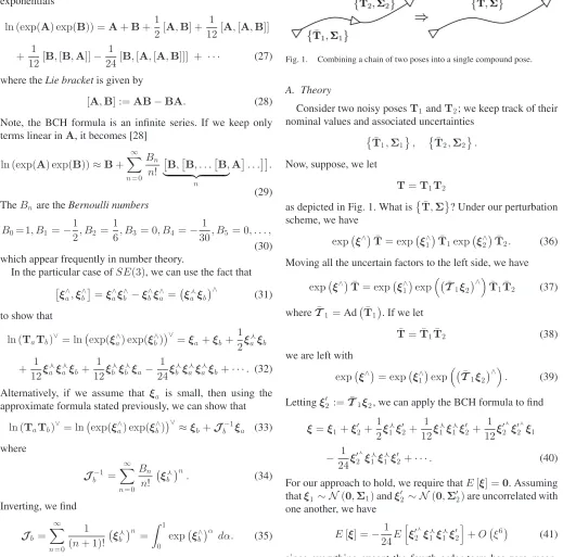
In this section, we investigate the problem of compounding two poses, each with associated uncertainty, as depicted in Fig. 1.
4There is also a right Jacobian if we instead assumeξ bis small.
Fig. 1. Combining a chain of two poses into a single compound pose.
A. Theory
Consider two noisy posesT1andT2; we keep track of their nominal values and associated uncertainties
¯
Now, suppose, we let
T=T1T2
Moving all the uncertain factors to the left side, we have
exp ξ∧T¯ = exp ξ∧1
we are left with
exp ξ∧= exp ξ∧1 one another, we have
E[ξ] =− 1 24E
ξ′2ξ1ξ1ξ′2+O ξ6 (41) since everything except the fourth-order term has zero mean. Thus, to third order, we can safely assume thatE[ξ] =0, and thus, (38) seems to be a reasonable way to compound the mean transformations.
It is also possible to show that the fourth-order term has zero mean,Eξ′2ξ1ξ1ξ′2=0, ifΣ1 is of the special form
The next task is to computeΣ=EξξT. Multiplying out to fourth order, we have
EξξT ≈E
where we have omitted showing any terms that have an odd power in either ξ1 or ξ′2 since these will by definition have expectation zero. This expression may look daunting, but we can take it term by term. To save space, we define and make use of the following two linear operators:
A:=−tr(A)1+A (44)
A,B:=AB+BA (45)
withA,B∈Rn×n. These provide the useful identity
−u∧Av∧≡ vuT,AT (46)
whereu,v∈R3andA∈R3×3. Making use of this repeatedly, we have out to fourth order
Eξ1ξT1
The resulting covariance is then
Σ4th ≈Σ1+Σ′2
additional fourth-order term s
(55)
correct to fourth order.5 This result is essentially the same as that of Wang and Chirikjian [26] but worked out for our slightly
5The sixth-order terms require a lot more work, but it is possible to compute them using Isserlis’ theorem.
different PDF, as discussed earlier; it is important to note that, while our method is fourth order in the perturbation variables, it is only second order in the covariance, which is the same as [26]. In summary, to compound two poses, we propagate the mean using (38) and the covariance using (55).
B. Sigmapoint Method
We can also make use of the popularsigmapoint transforma-tion[29] to pass uncertainty through the compound pose change. In this section, we tailor this to our specific type ofSE(3) per-turbation. Our approach to handling sigmapoints is quite similar to that taken by Hertzberget al.[15] as well as Brookshire and Teller [30]. In our case, we begin by approximating the joint input Gaussian using a finite number of samples,{T1,ℓ,T2,ℓ}
whereλis a user-definable scaling constant,6andL= 12. We
then pass each of these samples through the compound pose change and compute the difference from the mean
ξℓ = ln T1,ℓT2,ℓT¯−1
∨, ℓ= 1. . .2L.
(56)
These are combined to create the output covariance according to
Note that we have assumed that the output sigmapoint sam-ples have zero mean in this formula, to be consistent with our mean propagation. Interestingly, this turns out to be al-gebraically equivalent to the second-order method (from the previous section) for this particular nonlinearity, since the noise sources onT1andT2 are assumed to be uncorrelated.
C. Simple Compound Example
In this section, we present a simple qualitative example of pose compounding and in Section III-D, we carry out a more quantitative study on a different setup. To see the qualitative difference between the second- and fourth-order methods, let us consider the case of compounding transformations many times in a row
As discussed earlier, this can be viewed as a discrete-time inte-gration of theSE(3)kinematic equations, as in (25). To keep things simple, we make the following assumptions:
¯
T0 =1, ξ0 ∼ N(0,0) (59)
¯
T= ¯
C ¯r 0T 1
, ξ∼ N(0,Σ) (60)
¯
C=1, ¯r= ⎡
⎣
r
0 0
⎤
⎦, Σ=diag 0,0,0,0,0, σ2.(61)
Although this example uses our 3-D tools, it is confined to a plane for the purpose of illustration and ease of plotting; it corresponds to a rigid body moving along the x-axis but with some uncertainty only on the rotational velocity about the z-axis. This could model a unicycle robot driving in the plane with a constant translational speed and slightly uncertain rotational speed (centered about zero). We are interested in how the covariance matrix fills in over time.
According to the second-order scheme, we have
¯
TK =
⎡
⎢ ⎣
1 0 0 K r
0 1 0 0 0 0 1 0 0 0 0 1
⎤
⎥
⎦ (62)
ΣK
=
⎡
⎢ ⎢ ⎢ ⎢ ⎢ ⎣
0 0 0 0 0 0
0 K(K−1)(2K−1)
6 r
2σ2 0 0 0 −K(K−1) 2 rσ
2
0 0 0 0 0 0
0 0 0 0 0 0
0 0 0 0 0 0
0 −K(K−1)
2 rσ
2 0 0 0 K σ2
⎤
⎥ ⎥ ⎥ ⎥ ⎥ ⎦
(63)
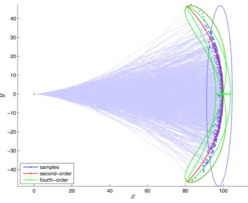
where we see that the top-left entry ofΣK, corresponding to uncertainty in thex-direction, does not have any growth of un-certainty. However, in the fourth-order scheme, the fill-in pattern is such that the top-left entry is nonzero. This happens for several reasons, but mainly through theBρρsubmatrix ofB. This leak-ing of uncertainty into an additional degree of freedom cannot be captured by keeping only the second-order terms. Fig. 2 pro-vides a numerical example of this effect. It shows that both the second- and fourth-order schemes do a good job of representing the ‘banana’-like distribution over poses, as discussed by Long et al. [31]. However, the fourth-order scheme has some finite uncertainty in the straight-ahead direction (as do the sampled trajectories), while the second-order scheme does not.
D. Compound Experiment
To quantitatively evaluate the pose-compounding techniques, we ran a second numerical experiment in which we compounded two poses including their associated covariance matrices
Fig. 2. Example of compoundingK= 100uncertain transformations (see Section III-C). The light blue lines and blue dots show 1000 individual sampled trajectories starting from(0,0)and moving nominally to the right at constant translational speed but with some uncertainty on the rotational velocity. The blue 1-sigma covariance ellipse is simply fitted to the blue samples to show what keepingxy-covariance relative to the start looks like. The red (second order) and green (fourth order) lines are the principal great circles of the 1-sigma covariance ellipsoid, given byΣK, mapped to thexyplane. Looking at the area(95,0), corresponding to straight ahead, the fourth-order scheme has some nonzero uncertainty (as do the samples), whereas the second-order scheme does not. We usedr= 1andσ= 0.03.
¯
T1:= exp
¯
ξ∧1, ξ¯1 := [ 0 2 0 π/6 0 0 ]T
Σ1:=α×diag
10,5,5,1
2,1, 1 2
¯
T2:= exp
¯
ξ∧2
, ξ¯2 := [ 0 0 1 0 π/4 0 ] T
Σ2:=α×diag
5,10,5,1
2, 1 2,1
whereα∈[0,1]is a scaling parameter that increases the mag-nitude of the input covariances parametrically.
We compounded these two poses according to (36), which re-sults in a mean ofT¯ = ¯T1T¯2. The covarianceΣwas computed using four methods.
1) Monte Carlo: We drew a large number,M = 1 000 000, of random samples (ξm1 andξm2) from the input covari-ance matrices, compounded the resulting transformations, and computed the covariance asΣm c = M1 %Mm= 1ξmξTm with Tm = exp ξ∧m1
¯
T1exp ξ∧m2
¯
T2, and ξm = ln TmT¯−1
∨
. This slow-but-accurate approach served as our benchmark to which the other three much faster methods were compared.
2) Second Order: We used the second-order method de-scribed previously to computeΣ2nd.
3) Fourth Order: We used the fourth-order method described previously to computeΣ4th.
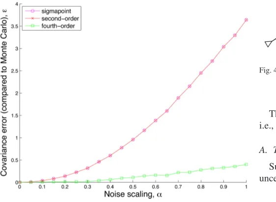
Fig. 3. Results from compound experiment (see Section III-D): Errorεin com-puting covariance associated with compounding two poses using three methods, as compared with Monte Carlo. The sigmapoint and second-order methods are algebraically equivalent for this problem and, thus, appear the same on the plot. The input covariances were gradually scaled up via the parameterα, highlight-ing the improved performance of the fourth-order method.
We compared each of the last three covariance matrices with the Monte Carlo one, using theFrobenius norm
ε:= &
tr(Σ−Σm c)T (Σ−Σm c)
.
Fig. 3 shows that for small input covariance matrices (i.e.,α
small), there is very little difference between the various meth-ods and the errors are all low compared with our benchmark. However, as we increase the magnitude of the input covariances, all the methods get worse, with the fourth-order method faring the best by about a factor of seven based on our error metric. Note, since αis scaling the covariance, the applied noise is increasing quadratically.
The second-order method and the sigmapoint method have indistinguishable performance, as they are algebraically equiv-alent. The fourth-order method goes beyond both of these by considering higher-order terms in the input covariance matri-ces. We did not compare the computational costs of the various methods as they are all extremely efficient, as compared with Monte Carlo.
It is also worth noting that our ability to correctly keep track of uncertainties onSE(3)decreases with increasing uncertainty. This can be seen directly in Fig. 3, as error increases with increasing uncertainty. This suggests that it may be wise to use only relative pose variables in order to keep uncertainties small; this idea was suggested early on by Brooks [5] and demonstrated recently by Sibley et al.[32]. If uncertainty must be tracked globally onSE(3), it may be necessary to move to an approach more along the lines of Leeet al.[24].
Fig. 4. CombiningKpose estimates into a single fused estimate.
IV. FUSINGPOSES
This section will investigate a different type of nonlinearity, i.e., the fusing of several pose estimates, as depicted in Fig. 4.
A. Theory
Suppose that we haveK estimates of a pose and associated uncertainties
¯
T1,Σ1
,T¯2,Σ2
, . . . ,T¯K,ΣK
. (64)
If we think of these as uncertain measurements of the true pose,
Ttrue, how can we optimally combine these into a single esti-mateT¯,Σ?
The vectorspace solution to fusion is straightforward and can be found exactly in closed form
¯
x=Σ
K
k= 1
Σ−k1x¯k, Σ= K
k= 1
Σ−k1
"−1
. (65)
The situation is somewhat more complicated when dealing with
SE(3), and we shall resort to an iterative scheme.
We define the error (that we will seek to minimize) asǫk ∼
N(0,Σk), which occurs between the individual estimate and the optimal estimateT¯⋆ so that
ǫk := ln T¯⋆T¯−k1∨= ln
exp ξ∧T¯T¯−k1
sm all
∨
= ln exp ξ∧exp ξ∧k ∨
(66)
where T¯ is our best guess so far,ξ is a small (unknown but optimal) perturbation between our best guess and the optimum, and
ξk := ln T¯T¯−k1∨ (67) is the difference between our best guess so far and each individ-ual estimate.
Applying the version of the BCH formula in (29), we have
ǫk ≈ξk +J−k1ξ (68)
correct to first order inξwith
J−1 k :=
∞
n= 0
Bn
n! ξ
k n
. (69)
utilizing the expression in (100) to computeJkanalytically and then invert. Theξk will be the residual errors after convergence.
We define the cost function that we want to minimize as
V :=1 2
K
k= 1
ǫTk Σ−k1ǫk
≈12
K
k= 1
ξk +J−k1ξTΣk−1 ξk +J−k1ξ
which is already quadratic in ξ. It is in fact a Mahalanobis distance[33], since we have chosen the weighting matrices to be the inverse covariance matrices; thus, minimizing V with respect toξis equivalent to maximizing the joint likelihood of the individual estimates. It is worth noting that because we are using a constraint-sensitive perturbation scheme, we do not need to worry about enforcing any constraints on our state variables during the optimization procedure. Taking the derivative with respect toξand setting to zero results in the following system of linear equations for the optimal value ofξ:
K
k= 1
J−kTΣ−k1J−k1
"
ξ=−
K
k= 1
J−kTΣ−k1ξk.
While this may look strange compared with (65), the Jacobian terms appear because our choice of error definition is in fact nonlinear owing to presence of the matrix exponentials. We then apply this optimal perturbation to our best guess so far
¯
T←exp ξ∧T¯
which ensuresT¯ remains inSE(3), and iterate to convergence. This optimization strategy was also used by Strasdatet al.[34], who argued that it avoids singularities in the representation of the mean,T¯, but retains a minimal parameterization during the optimization stepξ. At the last iteration, we take
Σ= K
k= 1
J−kTΣ−k1J−k1
"−1
for the covariance matrix. This approach has the form of a Gauss–Newton method.
This fusion problem is similar to the one investigated by Smithet al.[14], but they only discuss the K= 2 case. Our study is closer to that of Long et al. [31], who discuss the
N = 2case and derive closed-form expressions for the fused mean and covariance for an arbitrary number of individual mea-surements, K; however, they do not iterate their solution and they are tracking a slightly different PDF, as discussed earlier. Wolfeet al.[27] also discuss fusion at length, albeit again us-ing a slightly different PDF than us. They discuss noniterative methods of fusion for arbitraryKand show numerical results forK= 2. We believe our approach generalizes all of these pre-vious works by 1) allowing the number of individual estimates
K to be arbitrary, 2) keeping an arbitrary number of terms in the approximation of the inverse JacobianN, and 3) iterating to convergence via a Gauss–Newton style optimization method. Our approach may also be simpler to implement than some of these previous methods.
Fig. 5. Results from the fusion experiment (see Section IV-B). (Left) Average final cost functionV as a function of the number of termsN, kept inJ−1
k . (Right) Same for the root-mean-squared pose error with respect to the true pose. Both plots show there is benefit in keeping more than one term inJ−1
k . The datapoint that is denoted by ‘∞’ uses the analytical expression in (100) to keep all the terms in the expansion.
B. Fusion Experiment
To validate the pose fusion method from the previous section, we used a true pose given by
Ttrue:= exp ξ∧true
, ξtrue:= [ 1 0 0 0 0 π/6 ]T and then generated three random pose measurements
¯
T1 := exp ξ∧1
Ttrue, T¯2 := exp ξ∧2
Ttrue
¯
T3 := exp ξ∧3
Ttrue (70)
where
ξ1∼ N
0,diag
10,5,5,1
2,1, 1 2
ξ2∼ N
0,diag
5,15,5,1
2, 1 2,1
ξ3∼ N
0,diag
5,5,25,1,1
2, 1 2
. (71)
We then solved for the pose using our Gauss–Newton technique (iterating until convergence), using the initial conditionT¯ =1. We repeated this forN= 1. . .6, which is the number of terms kept inJ−k1in (103), shown later. We also used the expression given in (100), shown later, to computeJk analytically (and then inverted numerically) and this is denoted by ‘N =∞.’
Fig. 5 plots two performance metrics. First, it plots the final converged value of the cost function,Vm, averaged overM = 1000 random trials V := 1
M %M
m= 1Vm. Second, it plots the root-mean-squared pose error (with respect to the true pose) of our estimateT¯m, again averaged over the sameMrandom trials
ε:= ' ( ( ) 1
M
M
m= 1
εT
mεm, εm := ln TtrueT¯−m1 ∨
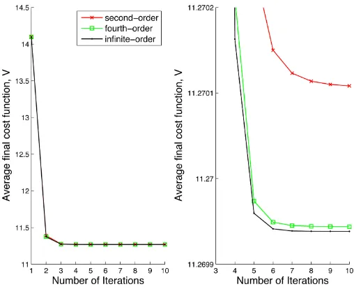
Fig. 6. Results from the fusion experiment. (Left) Convergence of the cost functionV with successive Gauss–Newton iterations. This is for just one of the
Mtrials that is used to generate Fig. 5. (Right) Same as left but zoomed in to show that theN= 2,4,∞solutions converge to progressively lower costs.
The plots show that both measures of error are monotonically reduced with increasingN. Moreover, we see that for this ex-ample, almost all of the benefit is gained with just four terms (or possibly even two). The results forN = 2,3are identical as are those forN = 4,5. This is because in the Bernoulli number sequence,B3 = 0andB5 = 0; therefore, these terms make no additional contribution toJ−k1in (103). It is also worth stating that if we make the rotational part of the covariances in (71) any bigger, we end up with a lot of samples that have rotated by more than angleπ, and this can be problematic for the performance metrics we are using.
Fig. 6 shows the convergence history of the cost, V, for a single random trial. The left side shows the strong benefit of iterating over the solution, while the right side shows that the cost converges to a lower value by keeping more terms in the approximation of J−k1 (cases N= 2,4,∞ shown). It would seem that takingN = 4for about seven iterations gains most of the benefit, for this example.
V. PROPAGATINGUNCERTAINTYTHROUGH ANONLINEAR
CAMERAMODEL
In estimation problems, we are often faced with passing un-certain quantities through nonlinear measurement models to produce expected measurements. Typically, this is carried out via linearization [35]. Sibley [36] shows how to carry out a second-order propagation for a stereo camera model account-ing for landmark uncertainty but not pose uncertainty. Here, we derive the full second-order expression for the mean (and co-variance) and compare this with Monte Carlo, the sigmapoint transformation, and linearization. We begin by discussing our representation of points and then present the Taylor-series ex-pansion of the measurement (camera) model followed by an experiment.
A. Homogeneous Points
Points in R3 can be represented using 4×1 homogeneous coordinates[3] as follows:
p= ⎡
⎢ ⎣
sx sy sz s
⎤
⎥ ⎦=
ε η
where s is some real, non-negative scalar, ε∈R3, and η is scalar. Whensis zero, it is not possible to convert back toR3, as this case represents points that are infinitely far away. Thus, homogeneous coordinates can be used to describe near and distant landmarks with no singularities or scaling issues [37]. They are also a natural representation in that points may then be transformed from one frame to another very easily using transformation matrices (e.g.,p2 =T21p1).
We will also make use of the following two operators7 to manipulate 4×1 columns
ε η
⊙
:=
η1 −ε∧ 0T 0T
,
ε η
⊚
:=
0 ε
−ε∧ 0
(72)
which result in a 4×6 and 6×4, respectively. With these defi-nitions, we have the following useful identities:
ξ∧p≡p⊙ξ, pTξ∧≡ξTp⊚ (73)
whereξ∈R6 andp∈R4, which will prove useful when ma-nipulating expressions involving points and poses together. We also have the identity
(Tp)⊙≡Tp⊙T−1 (74) which is similar to (108) and (109), shown later. To the best of our knowledge, these operators and identities have not previ-ously appeared in the literature.
To perturb points in homogeneous coordinates, we will oper-ate directly on thexyzcomponents by writing
p= ¯p+Dζ (75)
where ζ∈R3 is the perturbation and D is a dilation matrix given by
D:= ⎡
⎢ ⎣
1 0 0 0 1 0 0 0 1 0 0 0
⎤
⎥
⎦. (76)
We thus have thatE[p] = ¯pand that
E[(p−p¯)(p−p¯)T] =DE[ζζT]DT (77) with no approximation.
B. Taylor-Series Expansion of a Camera Model
It is common to linearize a nonlinear observation model for use in pose estimation. In this section, we show how to do a
more general Taylor-series expansion of such a model and work out the second-order case in detail. Our camera model will be
y=f(Tp) (78)
where T is the pose of the camera, and p is the position of a landmark (as a homogeneous point). The nonlinear function
f(·)maps homogeneous points in the camera frameTpto mea-surementsy. Our task will be to pass a Gaussian representation of the pose and landmark, given by {T,p,Ξ}, whereΞ is a 9×9 covariance for both quantities, through the camera model to produce a mean and covariance for the measurement{y,R}. We can think of this as the composition of two nonlinearities, one to transfer the landmark into the camera frame and one to produce the observations. We will treat each one in turn. If we change the pose of the camera and/or the position of the landmark a little bit, we have
Tp= exp ξ∧T¯ (¯p+Dζ)
≈
1+ξ∧+1 2ξ
∧ξ∧
¯
T(¯p+Dζ) (79) where we have kept the first two terms in the Taylor series for the pose perturbation. If we multiply out and continue to keep only those terms that are second order or lower inξandζ, we have
Tp≈g+Gθ+1 2
4
i= 1
θTGiθ
scalar
1i (80)
where1iis theith column of the 4×4 identity matrix, and
g:= ¯Tp¯ (81)
G:= [ T¯p¯⊙ TD¯ ] (82)
Gi:= 1⊚
i T¯p¯
⊙ 1⊚
i TD¯
1⊚i TD¯ T 0
(83)
θ:=
ξ ζ
. (84)
Arriving at these expressions requires repeated application of the identities in the previous section.
To then apply the nonlinear camera model, we use the chain rule (for first and second derivatives) so that
f(Tp)≈h+Hθ+1 2
J
j= 1
θT Hjθ
scalar
1j (85)
correct to second order inθ, where
h:=f(g) (86)
H:=FG, F := ∂f
∂g
g (87)
Hj :=GT FjG+ 4
i= 1
1TjF 1i scalar
Gi (88)
Fj := ∂ 2f
j
∂g∂gT
g (89)
jis an index over theJ rows off(·), and1j is thejth column of theJ×Jidentity matrix. The Jacobian off(·)isF, and the Hessian of thejth rowfj(·)isFj.
If we only care about the first-order perturbation, we simply have
f(Tp) =h+Hθ (90)
wherehandHare unchanged.
These perturbed measurement equations can then be used within any estimation scheme we like; in the next section, we will use these with a stereo camera model to show the benefit of the second-order terms.
C. Propagating Gaussian Uncertainty Through the Camera
Suppose that the input uncertainties, embodied byθ, are zero-mean, Gaussian
θ∼ N(0,Ξ) (91)
where we note that in general there could be correlations be-tween the poseTand the landmarkp.
Then, to first order, our measurement is given by
y1st=h+Hθ (92)
andy¯1st=E[y1st] =h, sinceE[θ] =0by assumption. The (second-order) covariance associated with the first-order camera model is given by
R2nd =E
(y1st−y¯1st) (y1st−y¯1st)T
=H Ξ HT. (93) For the second-order camera model, we have
y2nd =h+Hθ+ 1 2
J
j= 1
θT Hjθ1j (94)
and consequently
¯
y2nd =E[y2nd] =h+ 1 2
J
j= 1
tr(HjΞ)1j (95) which has an extra nonzero term as compared with the first-order camera model. The larger the input covarianceΞis, the larger this term can become, depending on the nonlinearity. For a linear camera model,Hj =0and the second- and first-order camera model means are identical.
We will also compute a (fourth-order) covariance, but with just second-order terms in the camera model expansion. To do this properly, we should expand the camera model to third order as there is an additional fourth-order covariance term involving the product of first- and third-order camera-model terms; how-ever, this would involve a complicated expression employing the third derivative of the camera model. As such, the approximate fourth-order covariance we will use is given by
R4th ≈E
(y2nd−y¯2nd) (y2nd −y¯2nd)T
=H Ξ HT −1
4 J
i= 1
tr(HiΞ)1i " ⎛
⎝ J
j= 1
tr(HjΞ)1j ⎞
+1 element ofΞ. The first- and third-order terms in the covari-ance expansion are identically zero owing to the symmetry of the Gaussian density. The last term in the above makes use of Isserlis’ theoremfor Gaussian variables
E[ξkξℓξmξn] =E[ξkξℓ]E[ξmξn] +E[ξkξm]E[ξℓξn] +E[ξkξn]E[ξℓξm].
D. Sigmapoint Method
Finally, we can also make use of the popular sigmapoint transformation [29] to pass uncertainty through the nonlinear camera model. As in the pose compounding problem, we tai-lor this to our specific type ofSE(3) perturbation. We begin by approximating the input Gaussian using a finite number of samples{Tℓ,pℓ}
SST :=Ξ, (Cholesky decomposition)
θℓ :=0
whereκis a user-definable constant,8andL= 9. We then pass each of these samples through the nonlinear camera model
yℓ =f(Tℓpℓ), ℓ= 0. . .2L.
These are combined to create the output mean and covariance according to
The next section will provide the details for a specific nonlinear camera modelf(·)representing a stereo camera.
E. Stereo Camera Model
To demonstrate the propagation of uncertainty through a non-linear measurement model,f(·), we will employ a stereo camera
8For all experiments in this paper, we usedκ= 0.
andfu, fv are the horizontal, vertical focal lengths (in pixels), (cu, cv)is the optical center of the images (in pixels), andbis the separation between the cameras (in meters). The optical axis of the camera is along thez-, orp3-, direction.
The Jacobian of this measurement model is given by
∂f
and the Hessian is given by
∂2f
where we have shown each component separately.
F. Camera Experiment
We used the following methods to pass a Gaussian uncertainty on camera pose and landmark position through the nonlinear stereo camera model.
1) Monte Carlo: We drew a large number M = 1000 000 of random samples from the input distribution, passed these through the camera model, and then computed the mean y¯m c and covariance Rm c. This slow-but-accurate approach served as our benchmark to which the other three much faster methods were compared.
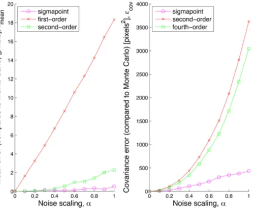
Fig. 7. Results from the stereo camera experiment (see Section V-F). (Left) Mean and (right) covariance errorsεm e a nandεc ovfor three methods of passing a Gaussian uncertainty through a nonlinear stereo camera model, as compared with Monte Carlo. The parameterαscales the magnitude of the input covariance matrix.
3) Second/Fourth Order:We used the second-order camera model to computey¯2ndandR4th, as described previously. 4) Sigmapoint:We used the sigmapoint method that has been
described previously to compute¯yspandRsp. The camera parameters were
b= 0.25m, fu =fv = 200pixels, cu =cv = 0pixels. We used the camera poseT:=1and let the landmark be located atp:= [ 10 10 10 1 ]T. For the combined pose/landmark uncertainty, we used an input covariance of
Ξ:=α×diag
1 10,
1 10,
1 10,
1 100,
1 100,
1
100,1,1,1
whereα∈[0,1]is a scaling parameter that allowed us to para-metrically increase the magnitude of the uncertainty.
To gauge the performance, we evaluated both the mean and covariance of each method by comparing the results to those of the Monte Carlo simulation according to the following metrics:
εm ean :=
(¯y−y¯m c)T(¯y−y¯m c)
εcov :=
tr((R−Rm c)T(R−Rm c)) where the latter is theFrobenius norm.
Fig. 7 shows the two performance metrics,εm ean andεcov, for each of the three techniques over a wide range of noise scalingsα. We see that the sigmapoint technique does the best on both mean and covariance. The second-order technique does reasonably well on the mean, but the corresponding fourth-order technique does poorly on the covariance (because of our inability to compute a fully fourth-order-accurate covariance, as explained earlier).
Fig. 8 provides a snapshot of a portion of the left image of the stereo camera with the mean and one-standard-deviation
Fig. 8. Results from the stereo camera experiment (see Section V-F). A portion of the left image of a stereo camera showing the mean and covariance (as a one-standard-deviation ellipse) for four methods of imaging a landmark with Gaussian uncertainty on the camera’s pose and the landmark’s position. This case corresponds to theα= 1datapoint in Fig. 7.
covariance ellipses shown for all techniques. We see that the sigmapoint technique does an excellent job on both the mean and the covariance, while the others do not fare as well.
We do not believe there has been another comparison of these methods of propagating uncertainty through a nonlinear camera model with uncertainty on the camera pose and landmark position, the closest being the work of Sibley [36].
VI. CONCLUSION
We have presented some generic techniques (and provided accompanying MATLAB scripts9) to associate uncertainty with 3-D pose (and landmark) variables and shown how to use these in three worked examples:
1) compounding two poses with associated uncertainties (to fourth order in our noise variables or second order in the associated covariances);
2) fusing multiple uncertain estimates of a pose (iteratively, to arbitrary order);
3) propagating uncertainty through a nonlinear camera model (to fourth order in our noise variables or second order in the associated covariances).
The general outcome is that depending on the application, dif-ferent methods have advantages, with the higher-order methods always doing better than the lower ones. The choice of whether to use a sigmapoint method to propagate uncertainty depends on
the application:nofor pose compounding butyesto propagate uncertainty through a nonlinear camera model.
The contributions of this paper are both the specific exam-ples as well as the detailed notation and identities to manipulate poses and associated uncertainties. Our use of the BCH for-mula in these manipulations, particularly our use of (29) and the tangible connection to theSE(3)Jacobian, is novel; this is important because it allows us to avoid unnecessarily introduc-ing the concept ofLie derivatives, and instead, we can simply manipulate perturbations representing noise variables. We be-lieve our comparison of the sigmapoint transformation to the Taylor-expansion methods to be new as well. Finally, the ap-pendix contains a few previously unpublished tidbits including a closed-form expression for theSE(3)Jacobian in terms of all of its constituent blocks.
We have been using these methods in several bundle-adjustment and pose-graph optimization problems for the past several years with good success. Looking forward, we believe these techniques could find application in other problems re-quiring detailed bookkeeping of pose uncertainties and, thus, hope others will find them useful.
APPENDIX
This Appendix contains additional notation and useful ex-pressions for implementation of key exex-pressions in this paper.
A. Useful Closed-Form Expressions
The matrix exponential to build a transformation can be eval-uated as
where the rightmost expression can be computed in closed form. To do so, we use the components ofξ= [φρ] to compute the rotation matrixC∈SO(3)
C:= exp φ∧= of rotation. We also compute
J:=
which is the (left)JacobianofSO(3). The inverse ofCis simply
C−1 =CT, and the inverse ofJis given by
Similar closed-form expressions can be found in [21] and [38]. We can also compute the Jacobian forSE(3)according to
J := The closed-form expression on the right can be populated using
Jabove and To the best of our knowledge, this last expression does not appear in the previous literature. The inverse ofJ is simply
J−1=
Bullo and Murray [39, eq. (2.21)] also discussJ−1, pointing out that the two diagonal blocks are indeedJ−1but do not work out the details of top-right block, which amounts to knowing the details ofQ.
B. Converting BetweenξandT
The detailed steps to convert (in closed form) between a
ξ∈R6 and aT∈SE(3)are provided as follows.
i) computing the rotation axisaas the eigenvec-tor corresponding to a unit eigenvalue of C
ii) solving for the rotation angle φ in tr(C) =
We were unable to find this direct proof in the literature and therefore provide it. Starting from the right-hand side, we have
exp ad ξ∧= exp ξ=
whereCis the usual expression in (97), and
K:=
which can be found through careful manipulation. Starting from the left-hand side, we have
Ad exp ξ∧=Ad where J is given in (98). Comparing (104) and (105), what remains to be shown is thatK= (Jρ)∧C. To see this, we use the following sequence of manipulations:
(Jρ)∧C= integrations by parts), and therefore,K≡(Jρ)∧C, concluding the proof.
D. Additional Useful Identities
Some more useful identities for SE(3) and se(3) are the following:
The authors would like to thank Prof. F. Dellaert at Georgia Tech and H. Sommer at ETH for many useful discussions during the preparation of this paper.
REFERENCES
[1] D. C. Brown, “A solution to the general problem of multiple station analytical stereotriangulation,” Patrick Air Force Base, Florida, RCA-MTP Data Reduction Tech. Rep. 43 (or AFMTC TR 58-8), 1958. [2] R. M. Murray, Z. Li, and S. Sastry,A Mathematical Introduction to
Robotic Manipulation. Boca Raton, FL, USA: CRC, 1994.
[3] R. Hartley and A. Zisserman,Multiple View Geometry in Computer Vision. Cambridge, U.K.: Cambridge Univ. Press, 2000.
[4] J. Stillwell,Naive Lie Theory. New York, NY, USA: Springer-Verlag, 2008.
[5] R. Brooks, “Visual map making for a mobile robot,” inProc. IEEE Int. Conf. Robot. Autom., Mar. 1985, vol. 2, pp. 824–829.
[6] R. C. Smith and P. Cheeseman, “On the representation and estimation of spatial uncertainty,”Int. J. Robot. Res., vol. 5, no. 4, pp. 56–68, 1986. [7] H. F. Durrant-Whyte, “Uncertain geometry in robotics,”IEEE J. Robot.
Autom., vol. 4, no. 1, pp. 23–31, Feb. 1988.
[8] R. C. Smith, M. Self, and P. Cheeseman, “Estimating uncertain spa-tial relationships in robotics,” inAutonomous Robot Vehicles, I. J. Cox and G. T. Wilfong, Eds. New York, NY, USA: Springer-Verlag, 1990, pp. 167–193.
[9] H. Durrant-Whyte and T. Bailey, “Simultaneous localisation and mapping (SLAM): Part I the essential algorithms,”IEEE Robot. Autom. Mag., vol. 11, no. 3, pp. 99–110, Jun. 2006.
[10] G. S. Chirikjian,Stochastic Models, Information Theory, and Li Groups: Classical Results and Geometric Methods. vol. 1, New York, NY, USA: Birkhauser, 2009.
[11] G. S. Chirikjian,Stochastic Models, Information Theory, and Li Groups: Analytic Methods and Modern Applications. vol. 2, New York, NY, USA: Birkhauser, 2009.
[12] S. F. Su and C. S. G. Lee, “Uncertainty manipulation and propagation and verification of applicability of actions in assembly tasks,” inProc. IEEE Int. Conf. Robot. Autom., 1991, vol. 3, pp. 2471–2476.
[13] S. F. Su and C. S. G. Lee, “Manipulation and propagation of uncertainty and verification of applicability of actions in assembly tasks,”IEEE Trans. Syst., Man Cybern., vol. 22, no. 6, pp. 1376–1389, Nov./Dec. 1992. [14] P. Smith, T. Drummond, and K. Roussopoulos, “Computing MAP
trajec-tories by representing, propagating, and combining PDFs over groups,” in Proc. IEEE Int. Conf. Comput. Vis., 2003, pp. 1275–1282.
[15] C. Hertzberg, R. Wagner, U. Frese, and L. Schr¨oder, “Integrating generic sensor fusion algorithms with sound state representations through encap-sulation of manifolds,”Inf. Fusion, vol. 14, no. 1, pp. 57–77, 2013. [16] S. Sastry, Nonlinear Systems: Analysis, Stability, and Control. New
York, NY, USA: Springer-Verlag, 1999.
[17] P. T. Furgale, “Extensions to the visual odometry pipeline for the explo-ration of planetary surfaces” Ph.D. dissertation, Dept. Aerosp. Eng., Univ. Toronto, Toronto, ON, Canada, 2011.
[18] P. C. Hughes,Spacecraft Attitude Dynamics. New York, NY, USA: Wi-ley, 1986.
[20] H. McKean,Stochastic Integrals. New York, NY, USA: Academic, 1969.
[21] F. C. Park, “The optimal kinematic design of mechanisms” Ph.D. disser-tation, Harvard Univ., Cambridge, MA, USA, 1991.
[22] G. M. T. D’Eleuterio, “Multibody dynamics for space station manipu-lators: Recursive dynamics of topological chains,” Dynacon Enterprises Ltd., Mississauga, ON, Canada, Tech. Rep. SS-3, Jun. 1985
[23] G. M. T. D’Eleuterio, “Dynamics of an elastic multibody chain: Part C— Recursive dynamics,”Dyn. Stabil. Syst., vol. 7, no. 2, pp. 61–89, 1992. [24] T. Lee, M. Leok, and N. H. McClamroch, “Global symplectic uncertainty
propagation on SO(3),” inProc. 47th IEEE Conf. Decision Control, 2008, pp. 61–66.
[25] Y. Wang and G. S. Chirikjian, “Error propagation on the Euclidean group with applications to manipulator kinematics,”IEEE Trans. Robot., vol. 22, no. 4, pp. 591–602, Aug. 2006.
[26] Y. Wang and G. S. Chirikjian, “Nonparametric second-order theory of error propagation on motion groups,”Int. J. Robot. Res., vol. 27, no. 11, pp. 1258–1273, 2008.
[27] K. Wolfe, M. Mashner, and G. Chirikjian, “Bayesian fusion on Lie groups,”J. Algebr. Statist., vol. 2, no. 1, pp. 75–97, 2011.
[28] S. Klarsfeld and J. A. Oteo, “The Baker-Campbell-Hausdorff formula and the convergence of the Magnus expansion,”J. Phys. A: Math. Gen., vol. 22, pp. 4565–4572, 1989.
[29] S. Julier and J. Uhlmann, “A general method for approximating nonlinear transformations of probability distributions,” Robotics Res. Group, Univ. Oxford, Oxford, U.K., Tech. Rep., 1996
[30] J. Brookshire and S. Teller, “Extrinsic calibration from per-sensor ego-motion,” presented at the Robot.: Sci. Syst. Conf., Sydney, Australia, Jul. 2012.
[31] A. W. Long, K. C. Wolfe, M. J. Mashner, and G. S. Chirikjian, “The ba-nana distribution is Gaussian: A localization study with exponential co-ordinates,” presented at the Robot.: Sci. Syst. Conf., Sydney, Australia, 2012.
[32] G. Sibley, C. Mei, I. Reid, and P. Newman, “Vast scale outdoor navigation using adaptive relative bundle adjustment,”Int. J. Robot. Res., vol. 29, no. 8, pp. 958–980, Jul. 2010.
[33] P. Mahalanobis, “On the generalized distance in statistics,” inProc. Nat. Inst. Sci., 1936, vol. 2, pp. 49–55.
[34] H. Strasdat, J. M. M. Montiel, and A. Davison, “Scale drift-aware large scale monocular SLAM,” presented at the Robot.: Sci. Syst. Conf., Zaragoza, Spain, Jun. 2010.
[35] L. Matthies and S. A. Shafer, “Error modeling in stereo navigation,”IEEE J. Robot. Autom., vol. RA-3, no. 3, pp. 239–248, Jun. 1987.
[36] G. Sibley, “Long range stereo data-fusion from moving platforms” Ph.D. dissertation, Dept. Comput. Sci., Univ. Southern California, Los Angeles, CA, USA, 2007.
[37] W. Triggs, P. McLauchlan, R. Hartley, and A. Fitzgibbon, “Bundle adjust-ment: A modern synthesis,” inVision Algorithms: Theory and Practice (LNCS series), W. Triggs, A. Zisserman, and R. Szeliski, Eds. New York, NY, USA: Springer-Verlag, 2000, pp. 298–375.
[38] F. C. Park, J. E. Bobrow, and S. R. Ploen, “A Lie group formulation of robot dynamics,”Int. J. Robot. Res., vol. 14, pp. 609–618, 1995. [39] F. Bullo and R. M. Murray, “Proportional derivative control on the
Eu-clidean group,” inProc. Eur. Control Conf., 1995, pp. 1091–1097.
Timothy D. Barfoot (M’10) received the Ph.D. degree from University of Toronto, Toronto, ON, Canada, in 2002.
He currently leads the Autonomous Space Robotics Lab, University of Toronto, which develops methods to allow mobile robots to operate in large-scale, unstructured, 3-D environments, using rich on-board sensing (e.g., cameras and laser rangefinders) and computation. He is also an Associate Professor with the University of Toronto Institute for Aerospace Studies, where he holds the Canada Research Chair (Tier II) in Autonomous Space Robotics and works in the area of guidance, navigation, and control of mobile robots for space and terrestrial applications. Prior to his current position, he spent four years at MDA Space Missions, where he developed autonomous vehicle navigation technologies for both planetary rovers and terrestrial applications such as underground mining.
Dr. Barfoot is an Ontario Early Researcher Award holder and a licensed Professional Engineer in the Province of Ontario.
Paul T. Furgale(M’11) received the B.A.Sc. de-gree in computer science from the University of Manitoba, Winnipeg, MB, Canada, in 2006 and the Ph.D. degree from the University of Toronto Institute for Aerospace Studies, Toronto, ON, Canada, 2011.