There are many algorithm texts that provide lots of well-polished code and proofs of correctness. Instead, this one presents insights, notations, and analogies to help the novice describe and think about algorithms like an expert. It is a bit like a carpenter studying hammers instead of houses. Jeff Edmonds provides both the big picture and easy step-by-step methods for developing algorithms, while avoiding the comon pitfalls. Paradigms such as loop invariants and recursion help to unify a huge range of algorithms into a few meta-algorithms. Part of the goal is to teach students to think abstractly. Without getting bogged down in formal proofs, the book fosters deeper understanding so that how and why each algorithm works is trans-parent. These insights are presented in a slow and clear manner accessible to second- or third-year students of computer science, preparing them to find on their own innovative ways to solve problems.
HOW TO THINK ABOUT
ALGORITHMS
Cambridge, New York, Melbourne, Madrid, Cape Town, Singapore, São Paulo
Cambridge University Press
The Edinburgh Building, Cambridge CB2 8RU, UK
First published in print format
ISBN-13 978-0-521-84931-9
ISBN-13 978-0-521-61410-8
ISBN-13 978-0-511-41370-4
© Jeff Edmonds 2008
2008
Information on this title: www.cambridge.org/9780521849319
This publication is in copyright. Subject to statutory exception and to the provision of
relevant collective licensing agreements, no reproduction of any part may take place
without the written permission of Cambridge University Press.
Cambridge University Press has no responsibility for the persistence or accuracy of urls
for external or third-party internet websites referred to in this publication, and does not
guarantee that any content on such websites is, or will remain, accurate or appropriate.
Published in the United States of America by Cambridge University Press, New York
www.cambridge.org
paperback
eBook (EBL)
Out of the Box Leaping Deep Thinking
Creative Abstracting Logical Deducing
with Friends Working Fun Having
Fumbling and Bumbling Bravely Persevering
Preface page xi
Introduction . . . . . 1
PART ONE. ITERATIVE ALGORITHMS AND LOOP INVARIANTS
1 Iterative Algorithms: Measures of Progress and Loop Invariants . . . . . 5 1.1 A Paradigm Shift: A Sequence of Actions vs. a Sequence of
Assertions 5
1.2 The Steps to Develop an Iterative Algorithm 8
1.3 More about the Steps 12
1.4 Different Types of Iterative Algorithms 21
1.5 Typical Errors 26
1.6 Exercises 27
2 Examples Using More-of-the-Input Loop Invariants . . . .29
2.1 Coloring the Plane 29
2.2 Deterministic Finite Automaton 31
2.3 More of the Input vs. More of the Output 39
3 Abstract Data Types . . . . 43
3.1 Specifications and Hints at Implementations 44
3.2 Link List Implementation 51
3.3 Merging with a Queue 56
3.4 Parsing with a Stack 57
4 Narrowing the Search Space: Binary Search . . . .60
4.1 Binary Search Trees 60
4.2 Magic Sevens 62
4.3 VLSI Chip Testing 65
4.4 Exercises 69
5 Iterative Sorting Algorithms . . . .71
viii
5.2 Counting Sort (a Stable Sort) 72
5.3 Radix Sort 75
5.4 Radix Counting Sort 76
6 Euclid’s GCD Algorithm . . . . 79
7 The Loop Invariant for Lower Bounds . . . . 85
PART TWO. RECURSION
8 Abstractions, Techniques, and Theory . . . .97
8.1 Thinking about Recursion 97
8.2 Looking Forward vs. Backward 99
8.3 With a Little Help from Your Friends 100
8.4 The Towers of Hanoi 102
8.5 Checklist for Recursive Algorithms 104
8.6 The Stack Frame 110
8.7 Proving Correctness with Strong Induction 112
9 Some Simple Examples of Recursive Algorithms . . . .114
9.1 Sorting and Selecting Algorithms 114
9.2 Operations on Integers 122
9.3 Ackermann’s Function 127
9.4 Exercises 128
10 Recursion on Trees . . . . 130
10.1 Tree Traversals 133
10.2 Simple Examples 135
10.3 Generalizing the Problem Solved 138
10.4 Heap Sort and Priority Queues 141
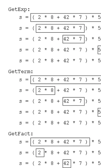
10.5 Representing Expressions with Trees 149
11 Recursive Images . . . .153
11.1 Drawing a Recursive Image from a Fixed Recursive and a Base
Case Image 153
11.2 Randomly Generating a Maze 156
12 Parsing with Context-Free Grammars . . . .159
PART THREE. OPTIMIZATION PROBLEMS
13 Definition of Optimization Problems . . . . 171
14 Graph Search Algorithms . . . . 173
14.1 A Generic Search Algorithm 174
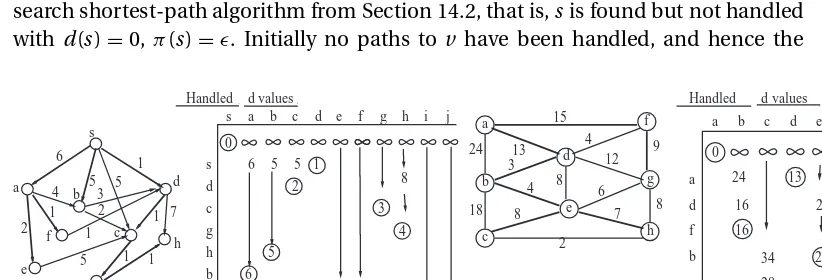
14.2 Breadth-First Search for Shortest Paths 179 14.3 Dijkstra’s Shortest-Weighted-Path Algorithm 183
14.4 Depth-First Search 188
14.5 Recursive Depth-First Search 192
14.6 Linear Ordering of a Partial Order 194
ix
15 Network Flows and Linear Programming . . . . 198
15.1 A Hill-Climbing Algorithm with a Small Local Maximum 200 15.2 The Primal–Dual Hill-Climbing Method 206 15.3 The Steepest-Ascent Hill-Climbing Algorithm 214
15.4 Linear Programming 219
15.5 Exercises 223
16 Greedy Algorithms . . . . 225
16.1 Abstractions, Techniques, and Theory 225
16.2 Examples of Greedy Algorithms 236
16.2.1 Example: The Job/Event Scheduling Problem 236 16.2.2 Example: The Interval Cover Problem 240 16.2.3 Example: The Minimum-Spanning-Tree Problem 244
16.3 Exercises 250
17 Recursive Backtracking . . . .251
17.1 Recursive Backtracking Algorithms 251
17.2 The Steps in Developing a Recursive Backtracking 256
17.3 Pruning Branches 260
17.4 Satisfiability 261
17.5 Exercises 265
18 Dynamic Programming Algorithms . . . . 267
18.1 Start by Developing a Recursive Backtracking 267 18.2 The Steps in Developing a Dynamic Programming Algorithm 271
18.3 Subtle Points 277
18.3.1 The Question for the Little Bird 278
18.3.2 Subinstances and Subsolutions 281
18.3.3 The Set of Subinstances 284
18.3.4 Decreasing Time and Space 288
18.3.5 Counting the Number of Solutions 291
18.3.6 The New Code 292
19 Examples of Dynamic Programs . . . .295
19.1 The Longest-Common-Subsequence Problem 295 19.2 Dynamic Programs as More-of-the-Input Iterative Loop
Invariant Algorithms 300
19.3 A Greedy Dynamic Program: The Weighted Job/Event
Scheduling Problem 303
19.4 The Solution Viewed as a Tree: Chains of Matrix Multiplications 306 19.5 Generalizing the Problem Solved: Best AVL Tree 311 19.6 All Pairs Using Matrix Multiplication 314
19.7 Parsing with Context-Free Grammars 315
x
20 Reductions and NP-Completeness . . . .324
20.1 Satisfiability Is at Least as Hard as Any Optimization Problem 326
20.2 Steps to Prove NP-Completeness 330
20.3 Example: 3-Coloring Is NP-Complete 338
20.4 An Algorithm for Bipartite Matching Using the Network
Flow Algorithm 342
21 Randomized Algorithms . . . . 346
21.1 Using Randomness to Hide the Worst Cases 347 21.2 Solutions of Optimization Problems with a Random Structure 350
PART FOUR. APPENDIX
22 Existential and Universal Quantifiers . . . .357
23 Time Complexity . . . . 366
23.1 The Time (and Space) Complexity of an Algorithm 366 23.2 The Time Complexity of a Computational Problem 371
24 Logarithms and Exponentials . . . . 374
25 Asymptotic Growth . . . .377
25.1 Steps to Classify a Function 379
25.2 More about Asymptotic Notation 384
26 Adding-Made-Easy Approximations . . . .388
26.1 The Technique 389
26.2 Some Proofs for the Adding-Made-Easy Technique 393
27 Recurrence Relations . . . .398
27.1 The Technique 398
27.2 Some Proofs 401
28 A Formal Proof of Correctness . . . .408
PART FIVE. EXERCISE SOLUTIONS . . . .411
Conclusion . . . . 437
To the Educator and the Student
This book is designed to be used in a twelve-week, third-year algorithms course. The goal is to teach students to think abstractly about algorithms and about the key algo-rithmic techniques used to develop them.
Meta-Algorithms: Students must learn so many algorithms that they are sometimes
overwhelmed. In order to facilitate their understanding, most textbooks cover the standard themes of iterative algorithms, recursion, greedy algorithms, and dynamic programming. Generally, however, when it comes to presenting the algorithms them-selves and their proofs of correctness, the concepts are hidden within optimized code and slick proofs. One goal of this book is to present a uniform and clean way of thinking about algorithms. We do this by focusing on the structure and proof of correctness ofiterativeandrecursivemeta-algorithms, and within these thegreedy anddynamic programmingmeta-algorithms. By learning these and their proofs of correctness, most actual algorithms can be easily understood. The challenge is that thinking about meta-algorithms requires a great deal of abstract thinking.
Abstract Thinking: Students are very good at learning
xii
Way of Thinking: People who develop algorithms have various ways of thinking and
intuition that tend not to get taught. The assumption, I suppose, is that these cannot be taught but must be figured out on one’s own. This text attempts to teach students to think like a designer of algorithms.
Not a Reference Book: My intention is not to teach a specific selection of algorithms for specific purposes. Hence, the book is not organized according to the application of the algorithms, but according to the techniques and abstractions used to develop them.
Developing Algorithms: The goal is not to present completed algorithms in a nice
clean package, but to go slowly through every step of the development. Many false starts have been added. The hope is that this will help students learn to develop al-gorithms on their own. The difference is a bit like the difference between studying carpentry by looking at houses and by looking at hammers.
Proof of Correctness: Our philosophy is not to follow an algorithm with a formal
proof that it is correct. Instead, this text is about learning how to think about, de-velop, and describe algorithms in such way that their correctness is transparent.
Big Picture vs. Small Steps: For each topic, I attempt both to give the big picture and to break it down into easily understood steps.
Level of Presentation: This material is difficult. There is no getting around that. I have tried to figure out where confusion may arise and to cover these points in more detail. I try to balance the succinct clarity that comes with mathematical formalism against the personified analogies and metaphors that help to provide both intuition and humor.
Point Form: The text is organized into blocks, each containing a title and a single
thought. Hopefully, this will make the text easier to lecture and study from.
Prerequisites: The text assumes that the students have completed a first-year
programming course and have a general mathematical maturity. The Appendix (Part Four) covers much of the mathematics that will be needed.
Homework Questions: A few homework questions are included. I am hoping to
de-velop many more, along with their solutions. Contributions are welcome.
Read Ahead: The student is expected to read the materialbeforethe lecture. This will facilitate productive discussion during class.
xiii the material over and over again out loud to yourself, to each other, and to your
stuffed bear.
Dreaming: I would like to emphasis the importance of
thinking, even daydreaming, about the material. This can be done while going through your day – while swim-ming, showering, cooking, or lying in bed. Ask ques-tions. Why is it done this way and not that way? In-vent other algorithms for solving a problem. Then look for input instances for which your algorithm gives the wrong answer. Mathematics is not all linear thinking.
If the essence of the material, what the questions are really asking, is allowed to seep down into your subconscious then with time little thoughts will begin to percolate up. Pursue these ideas. Sometimes even flashes of inspiration appear.
Acknowledgments
Introduction
From determining the cheapest way to make a hot dog to monitoring the workings of a factory, there are many complexcomputational problemsto be solved. Before executablecodecan be produced, computer scientists need to be able to design the
algorithmsthat lie behind the code, be able to understand and describe such algo-rithms abstractly, and be confident that they work correctly and efficiently. These are the goals of computer scientists.
A Computational Problem: A specification of a computational problem uses
pre-conditionsandpostconditionsto describe for each legalinput instancethat the com-putation might receive, what the required output or actions are. This may be a func-tion mapping each input instance to the required output. It may be an optimizafunc-tion problem which requires a solution to be outputted that is “optimal” from among a huge set of possible solutions for the given input instance. It may also be an ongoing system or data structure that responds appropriately to a constant stream of input.
Example:Thesortingproblem is defined as follows:
Preconditions: The input is a list ofnvalues, including possible repetitions.
Postconditions:The output is a list consisting of the samenvalues in non-decreasing order.
An Algorithm: Analgorithmis a step-by-step procedure which, starting with an
in-put instance, produces a suitable outin-put. It is described at the level of detail and ab-straction best suited to the human audience that must understand it. In contrast,
codeis an implementation of an algorithm that can be executed by a computer. Pseu-docodelies between these two.
An Abstract Data Type: Computers use zeros and ones, ANDs and ORs, IFs and
2
abstract operationssuch as “sort the list,” “pop the stack,” or “trace a path”; and ab-stract relationshipssuch as greater than, prefix, subset, connected, and child. To be useful, the nature of these objects and the effect of these operations need to be un-derstood. However, in order to hide details that are tedious or irrelevant, the precise implementations of these data structure and algorithms do not need to be specified. For more on this see Chapter 3.
Correctness: An algorithm for the problem iscorrectif for every legal input instance,
the required output is produced. Though a certain amount of logical thinking is re-quireds, the goal of this text is to teach how to think about, develop, and describe algorithms in such way that their correctness is transparent. See Chapter 28 for the formal steps required to prove correctness, and Chapter 22 for a discussion offorall
andexiststatements that are essential for making formal statements.
Running Time: It is not enough for a computation to eventually get the correct
answer. It must also do so using a reasonable amount of time and memory space. The running time of an algorithm is a function from the size n of the input in-stance given to a bound on the number ofoperationsthe computation must do. (See Chapter 23.) The algorithm is said to befeasibleif this function is apolynomiallike
Time(n)=(n2), and is said to beinfeasibleif this function is anexponentiallike
Time(n)=(2n). (See Chapters 24 and 25 for more on the asymptotics of functions.) To be able to compute the running time, one needs to be able to add up the times taken in each iteration of a loop and to solve the recurrence relation defining the time of a recursive program. (See Chapter 26 for an understanding ofn
i=1i=(n2), and Chapter 27 for an understanding ofT(n)=2T(n2)+n=(nlogn).)
Meta-algorithms: Most algorithms are best described as being either iterativeor
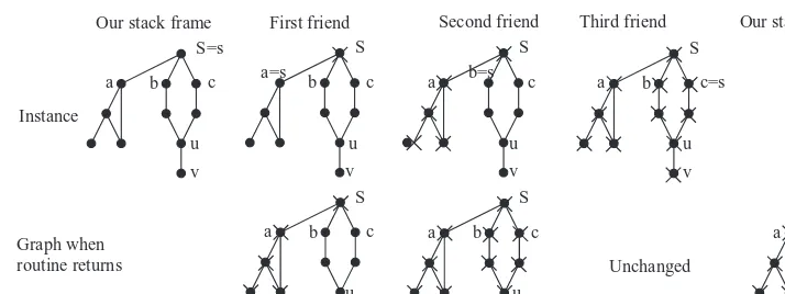
recursive. An iterative algorithm (Part One) takes one step at a time, ensuring that each step makesprogresswhile maintaining theloop invariant. A recursive algorithm (Part Two) breaks its instance into smaller instances, which it gets afriendto solve, and then combines their solutions into one of its own.
5
1
Iterative Algorithms: Measures of
Progress and Loop Invariants
Using an iterative algorithm to solve a computa-tional problem is a bit like following a road, possibly long and difficult, from your start location to your destination. With each iteration, you have a method that takes you a single step closer. To ensure that you move forward, you need to have ameasure of progress
telling you how far you are either from your starting location or from your destination. You cannot expect to know exactly where the algorithm will go, so you need to expect some weaving and winding. On the other hand, you do not want to have to know how to handle every ditch and dead end in the world. A compromise between these two is to have a loop invariant, which defines a road (or region) that you may not leave. As you travel, worry about one step
at a time. You must know how to get onto the road from any start location. From every place along the road, you must know what actions you will take in order to step forward while not leaving the road. Finally, when sufficient progress has been made along the road, you must know how to exit and reach your destination in a reasonable amount of time.
1.1 A Paradigm Shift: A Sequence of Actions vs. a Sequence of Assertions
6 One of the first important paradigm shifts
that programmers struggle to make is from viewing an algorithm as a sequence of actions to viewing it as a sequence of snapshots of the state of the computer. Programmers tend to fixate on the first view, because code is a sequence of instructions for action and a computation is a sequence of actions. Though this is an impor-tant view, there is another. Imagine stopping time at key points during the computation and taking still pictures of the state of the computer. Then a computation can equally be viewed as a sequence of such snapshots. Having two ways of viewing the same thing gives one both more tools to handle it and a deeper understanding of it. An example of viewing a computation as an alteration between assertions about the current state of the computation and blocks of actions that bring the state of the computation to the next state is shown here.
The Challenge of the Sequence-of-Actions View: Suppose one is designing a
new algorithm or explaining an algorithm to a friend. If one is thinking of it as se-quence of actions, then one will likely start at the beginning: Do this. Do that. Do this. Shortly one can get lost and not know where one is. To handle this, one simulta-neously needs to keep track of how the state of the computer changes with each new action. In order to know what action to take next, one needs to have a global plan of where the computation is to go. To make it worse, the computation has manyIFs and LOOPSso one has to consider all the various paths that the computation may take.
The Advantages of the Sequence of Snapshots View: This new paradigm is
useful one from which one can think about, explain, or develop an algorithm.
Pre- and Postconditions: Before one can consider an algorithm, one needs to
care-fully define the computational problem being solved by it. This is done with pre- and postconditions by providing the initial picture, orassertion, about the input instance and a corresponding picture or assertion about required output.
Start in the Middle: Instead of starting with the first line of code, an alternative way
7 Instead, it gives general properties and relationships between the various data
struc-tures that are key to understanding the algorithm. If this assertion is sufficiently gen-eral, it will capture not just this one point during the computation, but many similar points. Then it might become a part of a loop.
Sequence of Snapshots: Once one builds up a sequence of assertions in this way,
one can see the entire path of the computation laid out before one.
Fill in the Actions: These assertions are just static snapshots of the computation
with time stopped. No actions have been considered yet. The final step is to fill in actions (code) between consecutive assertions.
One Step at a Time: Each such block of actions can be executed completely
inde-pendently of the others. It is much easier to consider them one at a time than to worry about the entire computation at once. In fact, one can complete these blocks in any order one wants and modify one block without worrying about the effect on the others.
Fly In from Mars: This is how you should fill in the code between theith and the
i+1st assertions. Suppose you have just flown in from Mars, and absolutely the only thing you know about the current state of your computation is that theith assertion holds. The computation might actually be in a state that is completely impossible to arrive at, given the algorithm that has been designed so far. It is allowing this that provides independence between these blocks of actions.
Take One Step: Being in a state in which theith assertion holds, your task is simply
to write some simple code to do a few simple actions, that change the state of the computation so that thei+1st assertion holds.
Proof of Correctness of Each Step: The proof that your algorithm works can also
be done one block at a time. You need to prove that if time is stopped and the state of the computation is such that theith assertion holds and you start time again just long enough to execute the next block of code, then when you stop time again the state of the computation will be such that thei+1st assertion holds. This proof might be a formal mathematical proof, or it might be informal handwaving. Either way, the formal statement of what needs to be proved is as follows:
ith−assertion&codei ⇒ i+1st−assertion
Proof of Correctness of the Algorithm: All of these individual steps can be put
8
that first assertion holds. At some other point, we proved that if the first assertion holds and the second block of code is executed then the state of the computation will be such that second assertion holds. This was done for each block. All of these independently proved statements can be put together to prove that if initially the input instance meets the precondition and the entire code is executed, then in the end the state of the computation will be such that the postcondition has been met. This is what is required to prove that algorithm works.
1.2 The Steps to Develop an Iterative Algorithm
Iterative Algorithms: A good way to structure many computer programs is to store
the key information you currently know in some data structure and then have each iteration of the main loop take a step towards your destination by making a simple change to this data.
Loop Invariant: A loop invariant expresses important relationships among the
variables that must be true at the start of every iteration and when the loop termi-nates. If it is true, then the computation is still on the road. If it is false, then the algorithm has failed.
The Code Structure: The basic structure of the code is as follows.
begin routine pre-cond
codepre-loop % Establish loop invariant
loop
loop-invariant exit whenexit-cond
codeloop % Make progress while maintaining the loop invariant
end loop
codepost-loop % Clean up loose ends
post-cond end routine
Proof of Correctness: Naturally, you want to be sure your algorithm will work on
all specified inputs and give the correct answer.
Running Time: You also want to be sure that your algorithm completes in a
reason-able amount of time.
The Most Important Steps: If you need to design an algorithm, do not start by
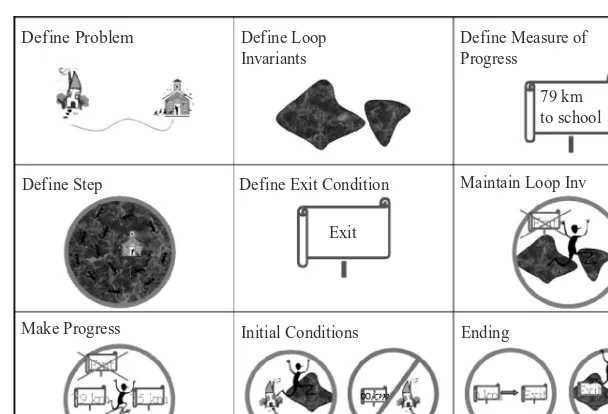
9 Define Problem Define Loop
Invariants
Define Step
Make Progress Initial Conditions Ending Exit
Define Exit Condition Maintain Loop Inv Define Measure of Progress
79 km to school
Figure 1.1: The requirements of an iterative algorithm.
together in very subtle ways. You may have to cycle through them a number of times, adjusting what you have done, until they all fit together as required.
1) Specifications: What problem are you solving? What are its pre- and
postcon-ditions—i.e., where are you starting and where is your destination?
2) Basic Steps: What basic steps will head you more or less in the correct direction?
3) Measure of Progress:You must define a measure of progress: where are the mile
markers along the road?
4) The Loop Invariant: You must define a loop invariant that will give a picture of
the state of your computation when it is at the top of the main loop, in other words, define the road that you will stay on.
5) Main Steps: For every location on the road, you must write the pseudocode
codeloopto take a single step. You do not need to start with the first location. I
rec-ommend first considering a typical step to be taken during the middle of the compu-tation.
6) Make Progress: Each iteration of your main step must make progress according
to your measure of progress.
7) Maintain Loop Invariant: Each iteration of your main step must ensure that the
loop invariant is true again when the computation gets back to the top of the loop. (Induction will then prove that it remains true always.)
8) Establishing the Loop Invariant: Now that you have an idea of where you are
10
codepre-loopto initially establish the loop invariant. How do you get from your house
onto the correct road?
9) Exit Condition: You must write the conditionexit-condthat causes the
compu-tation to break out of the loop.
10) Ending: How does the exit condition together with the invariant ensure that the
problem is solved? When at the end of the road but still on it, how do you produce the required output? You must write the pseudocodecodepost-loopto clean up loose ends
and to return the required output.
11) Termination and Running Time: How much progress do you need to make
be-fore you know you will reach this exit? This is an estimate of the running time of your algorithm.
12) Special Cases: When first attempting to design an algorithm, you should only
consider one general type of input instances. Later, you must cycle through the steps again considering other types of instances and special cases. Similarly, test your al-gorithm by hand on a number of different examples.
13) Coding and Implementation Details: Now you are ready to put all the pieces
to-gether and produce pseudocode for the algorithm. It may be necessary at this point to provide extra implementation details.
14) Formal Proof: If the above pieces fit together as required, then your algorithm
works.
EXAMPLE 1.2.1 The Find-Max Two-Finger Algorithm
to Illustrate These Ideas
1) Specifications: An input instance consists of a listL(1..n) of elements. The output consists of an indexisuch thatL(i) has maximum value. If there are multiple entries with this same value, then any one of them is returned.
2) Basic Steps: You decide on the two-finger method. Your right finger runs down the list.
3) Measure of Progress: The measure of progress is how far along the list your right finger is.
4) The Loop Invariant: The loop invariant states that your left finger points to one of the largest entries encountered so far by your right finger.
11
6) Make Progress: You make progress because your right finger moves one entry.
7) Maintain Loop Invariant: You know that the loop invariant has been maintained as follows. For each step, the new left finger element is Max(old left finger element, new element). By the loop invariant, this is Max(Max(shorter list), new element). Mathe-matically, this is Max(longer list).
8) Establishing the Loop Invariant: You initially establish the loop invariant by point-ing both fpoint-ingers to the first element.
9) Exit Condition: You are done when your right finger has finished traversing the list.
10) Ending:In the end, we know the problem is solved as follows. By the exit condi-tion, your right finger has encountered all of the entries. By the loop invariant, your left finger points at the maximum of these. Return this entry.
11) Termination and Running Time: The time required is some constant times the
length of the list.
12) Special Cases: Check what happens when there are multiple entries with the
same value or whenn=0 orn=1.
13) Coding and Implementation Details: algorithm Find Max(L)
pre-cond: Lis an array ofnvalues.
post-cond: Returns an index with maximum value. begin
i=1; j=1 loop
loop-invariant: L[i] is max inL[1..j]. exit when (j ≥n)
% Make progress while maintaining the loop invariant j = j+1
if(L[i]<L[j] ) theni=j end loop
return(i) end algorithm
14) Formal Proof: The correctness of the algorithm follows from the above steps.
A New Way of Thinking: You may be tempted to believe that measures of progress
12
essential. The description of the preceding algorithms and their proofs of correctness are wrapped up into one.
Keeping Grounded: Loop invariants constitute a life philosophy. They lead to
feel-ing grounded. Most of the code I mark as a teacher makes me feel ungrounded. It cycles, but I don’t know what the variables mean, how they fit together, where the algorithm is going, or how to start thinking about it. Loop invariants mean starting my day at home, where I know what is true and what things mean. From there, I have enough confidence to venture out into the unknown. However, loop invariants also mean returning full circle to my safe home at the end of my day.
EXERCISE 1.2.1 What are the formal mathematical things involving loop invariants that must be proved, to prove that if your program exits then it obtains the postcondi-tion?
1.3 More about the Steps
In this section I give more details about the steps for developing an iterative algo-rithm.
1) Specifications: Before we can design an iterative algorithm, we need to know
precisely what it is supposed to do.
Preconditions: What are the legal input instances? Any assertions that are promised to be true about the input instance are referred to aspreconditions.
Postconditions: What is the required output for each legal instance? Any asser-tions that must be true about the output are referred to aspostconditions.
Correctness: An algorithm for the problem iscorrectif for every legal input in-stance, the required output is produced. If the input instance does not meet the preconditions, then all bets are off. Formally, we express this as
pre-cond&codealg ⇒ post-cond This correctness is only with respect to the specifications.
Example:Thesortingproblem is defined as follows:
Preconditions: The input is a list ofnvalues, including possible repeatations.
Postconditions:The output is a list consisting of the samenvalues in non-decreasing order.
13 Implementer: When you are writing a subroutine, you can assume the input
comes to your program in the correct form, satisfying all the preconditions. You must write the subroutine so that it ensures that the postconditions hold after execution.
User:When you are using the subroutine, you must ensure that the input you provide meets the preconditions of the subroutine. Then you can trust that the output meets its postconditions.
2) Basic Steps: As a preliminary to designing the algorithm it can be helpful to
con-sider what basic steps or operations might be performed in order to make progress towards solving this problem. Take a few of these steps on a simple input instance in order to get some intuition as to where the computation might go. How might the information gained narrow down the computation problem?
3) Measure of Progress: You need to define a function that, when given the
cur-rent state of the computation, returns an integer value measuring either how much progress the computation has already made or how much progress still needs to be made. This is referred to either as ameasure of progressor as apotential function. It must be such that the total progress required to solve the problem is not infinite and that at each iteration, the computation makes progress. Beyond this, you have com-plete freedom to define this measure as you like. For example, your measure might state the amount of the output produced, the amount of the input considered, the extent to which the search space has been narrowed, some more creative function of the work done so far, or how many cases have been tried. Section 1.4 outlines how these different measures lead to different types of iterative algorithms.
4) The Loop Invariant: Often, coming up with the loop invariant is the hardest
part of designing an algorithm. It requires practice, perseverance, creativity, and in-sight. However, from it the rest of the algorithm often follows easily. Here are a few helpful pointers.
Definition: Aloop invariantis an assertion that is placed at the top of a loop and that must hold true every time the computation returns to the top of the loop.
14
to a loop that is executed many times or to an object-oriented data structure that has an ongoing life.
Designing, Understanding, and Proving Correct:Generally, assertions are not tasks for the algorithm to perform, but are only comments that are added to assist the designer, the implementer, and the reader in understanding the algorithm and its correctness.
Debugging:Some languages allow you to insert assertions as lines of code. If during the execution such an assertion is false, then the program automati-cally stops with a useful error message. This is helpful both when debugging and after the code is complete. It is what is occurring when an error box pops up during the execution of a program telling you to contact the vendor if the error persists. Not all interesting assertions, however, can be tested feasibly within the computation itself.
Picture from the Middle: A loop invariant should describe what you would like the data structure to look like when the computation is at the beginning of an iteration. Your description should leave your reader with a visual image. Draw a picture if you like.
Don’t Be Frightened:A loop invariant need not consist of formal mathematical mumbo jumbo if an informal description gets the idea across better. On the other hand, English is sometimes misleading, and hence a more mathematical lan-guage sometimes helps. Say things twice if necessary. I recommend pretending that you are describing the algorithm to a first-year student.
On the Road: A loop invariant must ensure that the computation is still on the road towards the destination and has not fallen into a ditch or landed in a tree.
A Wide Road: Given a fixed algorithm on a fixed input, the computation will fol-low one fixed line. When the algorithm designer knows exactly where this line will go, he can use a very tight loop invariant to define a very narrow road. On the other hand, because your algorithm must work for an infinite number of input instances and because you may pass many obstacles along the way, it can be dif-ficult to predict where the computation might be in the middle of its execution. In such cases, using a very loose loop invariant to define a very wide road is com-pletely acceptable. The line actually followed by the computation might weave and wind, but as long as it stays within the boundaries of the road and continues to make progress, all is well. An advantage of a wide road is that it gives more flexibility in how the main loop is implemented. A disadvantage is that there are then more places where the computation might be, and for each the algorithm must define how to take a step.
15 left finger should point at when there are a number of entries with the same
maximum value.
Meaningful and Achievable: You want a loop invariant that ismeaningful, mean-ing it is strong enough that, with an appropriate exit condition, it will guarantee the postcondition. You also want the loop invariant to beachievable, meaning you can establish and maintain it.
Know What a Loop Invariant Is: Be clear about what a loop invariant is. It is not code, a precondition, a postcondition, or some other inappropriate piece of in-formation. For example, stating something that is always true, such as “1+1= 2” or “The root is the max of any heap,” may be useful information for the answer to the problem, but should not be a part of the loop invariant.
Flow Smoothly:The loop invariant should flow smoothly from the begin-ning to the end of the algorithm.
r At the beginning, it should follow
easily from the preconditions.
r It should progress in small natural
steps.
r Once the exit condition has been
met, the postconditions should easily follow.
Ask for 100%: A good philosophy in life is to ask for 100% of what you want, but not to assume that you will get it.
Dream: Do not be shy. What would you like to be true in the middle of your computation? This may be a reasonable loop invariant, and it may not be.
Pretend:Pretend that a genie has granted your wish. You are now in the mid-dle of your computation, and your dream loop invariant is true.
Maintain the Loop Invariant: From here, are you able to take some compu-tational steps that will make progress while maintaining the loop invariant? If so, great. If not, there are two common reasons.
Too Weak:If your loop invariant is too weak, then the genie has not pro-vided you with everything you need to move on.
Too Strong: If your loop invariant is too strong, then you will not be able to establish it initially or maintain it.
16
state. As a check, pretend that you are a Martian who has jumped into the top of the loop knowingnothingthat is not stated in the loop invariant.
Example:In the find-max two-finger algorithm, the loop in-variant does make some unstated assumptions. It assumes that the numbers above your right finger have been en-countered by your right finger and those below it have not. Perhaps more importantly for,±1 errors, is whether or not the number currently being pointed has been encountered
already. The loop invariant also assumes that the numbers in the list have not changed from their original values.
A Starry Night: How did van Gogh come up with his famous painting,A Starry Night? There’s no easy answer. In the same way, coming up with loop invariants and algorithms is an art form.
Use This Process: Don’t come up with the loop invariant after the fact. Use it to design your algorithm.
5) Main Steps: The pseudocodecodeloopmust be defined so that it can be taken
not just from where you think the computation might be, but from any state of the data structure for which the loop invariant is true and the exit condition has not yet been met.
Worry aboutone step at a time. Don’t get pulled into the strong desire to under-stand the entire computation at once. Generally, this only brings fear and unhap-piness. I repeat the wisdom taught by both the Buddhists and the twelve-step pro-grams: Today you may feel like like you were dropped off in a strange city without knowing how you got there. Do not worry about the past or the future. Be reassured that you are somewhere along the correct road. Your goal is only to take one step so that you make progress and stay on the road. Another analogy is to imagine you are part of a relay race. A teammate hands you the baton. Your job is only to carry it once around the track and hand it to the next teammate.
6) Make Progress: You must prove that progress of at least one unit of your
mea-sure is made every time the algorithm goes around the loop. Sometimes there are odd situations in which the algorithm can iterate without making any measurable progress. This is not acceptable. The danger is that the algorithm will loop forever. You must either define another measure that better shows how you are making progress during such iterations or change the step taken in the main loop so that progress is made. The formal proof of this is similar to that for maintaining the loop invariant.
7) Maintain the Loop Invariant: You must prove that the loop invariant is
17 The Formal Statement: Whether or not you want to prove it formally, the formal
statement that must be true is
loop-invariant′¬exit-cond&codeloop ⇒ loop-invariant′′ Proof Technique:
r Assume that the computation is at the top of the loop.
r Assume that the loop invariant is satisfied; otherwise the program would have
already failed. Refer back to the picture that you drew to see what this tells you about the current state of the data structure.
r You can also assume that the exit condition is not satisfied, because otherwise
the loop would exit.
r Execute the pseudocodecode
loop, in one iteration of the loop. How does this
change the data structure?
r Prove that when you get back to the top of the loop again, the requirements set
by the loop invariant are met once more.
Different Situations: Many subtleties can arise from the huge number of differ-ent input instances and the huge number of differdiffer-ent places the computation might find itself in.
r I recommend first designing the pseudocodecode
loop to work for a general
middle iteration when given a large and general input instance. Is the loop in-variant maintained in this case?
r Then try the first and last couple of iterations.
r Also try special case input instances. Before writing separate code for these,
check whether the code you already have happens to handle these cases. If you are forced to change the code, be sure to check that the previously handled cases still are handled.
r To prove that the loop invariant is true in all situations, pretend that you are
at the top of the loop, but you do not know how you got there. You may have dropped in from Mars. Besides knowing that the loop invariant is true and the exit condition is not, you know nothing about the state of the data structure. Make no other assumptions. Then go around the loop and prove that the loop invariant is maintained.
Differentiating between Iterations: The assignmentx=x+2 is meaningful as a line of code, but not as a mathematical statement. Definex′to be the value of
xat the beginning of the iteration andx′′ that after going around the loop one
more time. The effect of the codex=x+2 is thatx′′ =x′+2.
8) Establishing the Loop Invariant: You must prove that the initial code
estab-lishes the loop invariant.
The Formal Statement: The formal statement that must be true is
18
Proof Technique:
r Assume that you are just beginning the computation.
r You can assume that the input instance satisfies the precondition; otherwise
you are not expected to solve the problem.
r Execute the codecode
pre-loopbefore the loop.
r Prove that when you first get to the top of the loop, the requirements set by the
loop invariant are met.
Easiest Way: Establish the loop invariant in the easiest way possible. For exam-ple, if you need to construct a set such that all the dragons within it are purexam-ple, the easiest way to do it is to construct the empty set. Note that all the dragons in this set are purple, because it contains no dragons that are not purple.
Careful: Sometimes it is difficult to know how to set the variables to make the loop invariant initially true. In such cases, try setting them to ensure that it is true after the first iteration. For example, what is the maximum value within an empty list of values? One might think 0 or∞. However, a better answer is−∞. When adding a new value, one uses the codenewMax=max(oldMax, newValue). Start-ing witholdMax= −∞, gives the correct answer when the first value is added.
9) Exit Condition: Generally you exit the loop when you have completed the task.
Stuck: Sometimes, however, though your intuition is that your algorithm de-signed so far is making progress each iteration, you have no clue whether, head-ing in this direction, the algorithm will ever solve the problem or how you would know it if it happens. Because the algorithm cannot make progress forever, there must be situations in which your algorithm gets stuck. For such situations, you must either think of other ways for your algorithm to make progress or have it exit. A good first step is to exit. In step 10, you will have to prove that when your algorithm exits, you actually are able to solve the problem. If you are unable to do this, then you will have to go back and redesign your algorithm.
Loop While vs Exit When: The following are equivalent: while(AandB)
. . . end while
loop
loop-invariant
exit when (notAor notB) . . .
end loop
19
10) Ending: In this step, you must ensure that once the loop has exited you will be
able to solve the problem.
The Formal Statement: The formal statement that must be true is
loop-invariant&exit-cond&codepost-loop ⇒ post-cond
Proof Technique:
r Assume that you have just broken out of the loop.
r You can assume that the loop invariant is true, because you have maintained
that it is always true.
r You can also assume that the exit condition is true by the fact that the loop has
exited.
r Execute the codecode
post-loopafter the loop to give a few last touches towards
solving the problem and to return the result.
r From these facts alone, you must be able to deduce that the problem has been
solved correctly, namely, that the postcondition has been established.
11) Termination and Running Time: You must prove that the algorithm does not
loop forever. This is done by proving that if the measure of progress meets some stated amount, then the exit condition has definitely been met. (If it exits earlier than this, all the better.) The number of iterations needed is then bounded by this stated amount of progress divided by the amount of progress made each iteration. The run-ning time is estimated by adding up the time required for each of these iterations. For some applications, space bounds (i.e., the amount of memory used) may also be im-portant. We discuss important concepts related to running time in Chapters 23–26: time and space complexity, the useful ideas of logarithms and exponentials, BigOh (O) and Theta () notation and several handy approximations.
12) Special Cases: When designing an algorithm, you do not want to worry about
every possible type of input instance at the same time. Instead, first get the algorithm to work for one general type, then another and another. Though the next type of in-put instances may require separate code, start by tracing out what the algorithm that you have already designed would do given such an input. Often this algorithm will just happen to handle a lot of these cases automatically without requiring separate code. When adding code to handle a special case, be sure to check that the previously handled cases still are handled.
13) Coding and Implementation Details: Even after the basic algorithm is
20
have chosen. This text does not focus on coding details. This does not mean that they are not important.
14) Formal Proof: Steps 1–11 are enough to ensure that your iterative algorithm
works, that is, that it gives the correct answer on all specified inputs. Consider some instance which meets the preconditions. By step 8 we establish the loop invariant the first time the computation is at the top of the loop, and by step 7 we maintain it each iteration. Hence by way of induction, we know that the loop invariant is true every time the computation is at the top of the loop. (See the following discussion.) Hence, by step 5, the step taken in the main loop is always defined and executes without crashing until the loop exits. Moreover, by step 6 each such iteration makes progress of at least one. Hence, by step 11, the exit condition is eventually met. Step 10 then gives that the postcondition is achieved, so that the algorithm works in this instance.
Mathematical Induction: Induction is an extremely important mathematical technique for proving universal statements and is the cornerstone of iterative algorithms. Hence, we will consider it in more detail.
Induction Hypothesis: For eachn≥0, letS(n) be the statement “If the loop has not yet exited, then the loop invariant is true when you are at the top of the loop after going aroundntimes.”
Goal:The goal is to prove that∀n≥0, S(n), namely, “As long as the loop has not yet exited, the loop invariant is always true when you are at the top of the loop.”
Proof Outline: Proof by induction onn.
Base Case:ProvingS(0) involves proving that the loop invariant is true when the algorithm first gets to the top of the loop. This is achieved by proving the statementpre-cond&codepre-loop⇒ loop-invariant.
Induction Step: Proving S(n−1)⇒S(n) involves proving that the loop invariant is maintained. This is achieved by proving the statement loop-invariant′& notexit-cond&codeloop⇒ loop-invariant′′.
Conclusion: By way of induction, we can conclude that∀n≥0, S(n), i.e., that the loop invariant is always true when at the top of the loop.
The Process of Induction:
S(0) is true (by base case)
S(0)⇒S(1) (by induction step,n=1)
hence,S(1) is true
S(1)⇒S(2) (by induction step,n=2)
hence,S(2) is true
21 Other Proof Techniques: Other formal steps for proving correctness are
de-scribed in Chapter 28.
Faith in the Method: Convince yourself that these steps are sufficient to define an
algorithm so that you do not have reconvince yourself every time you need to design an algorithm.
1.4 Different Types of Iterative Algorithms
To help you design a measure of progress and a loop invariant for your algorithm, here are a few classic types, followed by examples of each type.
More of the Output: If the solution is a structure composed of many pieces (e.g.,
an array of integers, a set, or a path), a natural thing to try is to construct the solution one piece at a time.
Measure of Progress: The amount of the output constructed.
Loop Invariant: The output constructed so far is correct.
More of the Input:Suppose the input consists ofnobjects (e.g., an array ofn
inte-gers or a graph withnnodes). It would be reasonable for the algorithm to read them in one at a time.
Measure of Progress: The amount of the input considered.
Loop Invariant: Pretending that this prefix of the input is the entire input, I have a complete solution.
Examples: Afteriiterations of the preceding find-max two-finger algorithm, the left finger points at the highest score within the prefix of the list seen so far. After
iiterations of one version of insertion sort, the firstielements of the input are sorted. See Figure 1.2.
22
Bad Loop Invariant: A common mistake is to give the loop invariant “I have han-dled and have a solution for each of the firstiobjects in the input.” This is wrong because each object in the input does not need a separate solution; the input as a whole does. For example, in the find-max two-finger algorithm, one cannot know whether one element is the maximum by considering it in isolation from the other elements. An element is only the maximum in comparison with the other elements in the sublist.
Narrowing the Search Space: If you are searching for something, try narrowing
the search space, maybe decreasing it by one or, even better, cutting it in half.
Measure of Progress: The size of the space in which you have narrowed the search.
Loop Invariant: If the thing being searched for is anywhere, then then it is in this narrowed sublist.
Example:Binary search.
Work Done: The measure of progress might also be some other more creative
func-tion of the work done so far.
Example:Bubble sort measures its progress by how many pairs of elements are out of order.
Case Analysis: Try the obvious thing. For which input instances does it work, and
for which does it not work? Now you only need to find an algorithm that works for those later cases. An measure of progress might include which cases you have tried.
We will now give a simple examples of each of these. Though you likely know these al-gorithms already, use them to understand these different types of iterative alal-gorithms and to review the required steps.
EXAMPLE 1.4.1 More of the Output—Selection Sort
1) Specifications: The goal is to rearrange a list ofnvalues in nondecreasing order.
2) Basic Steps: We will repeatedly select the smallest unselected element.
3) Measure of Progress: The measure of progress is the number k of elements
se-lected.
23
5) Main Steps: The main step is to find the smallest element from among those in the remaining set of larger elements and to add this newly selected element to the end of the sorted list of elements.
6) Make Progress: Progress is made becausekincreases.
7) Maintain Loop Invariant: We must prove that loop-invariant′ & not exit− cond & codeloop ⇒ loop-invariant′′. By the previous loop invariant, the newly
selected element is at least the size of the previously selected elements. By the step, it is no bigger than the elements on the side. It follows that it must be thek+1st element in the list. Hence, moving this element from the set on the side to the end of the sorted list ensures that the selected elements in the new list are thek+1 smallest and are sorted.
8) Establishing the Loop Invariant: We must prove thatpre-cond&codepre-loop⇒ loop-invariant. Initially,k=0 are sorted and all the elements are set aside.
9) Exit Condition: Stop whenk=n.
10) Ending:We must prove loop-invariant & exit-cond & codepost-loop ⇒ post-cond. By the exit condition, all the elements have been selected, and by the loop invariant these selected elements have been sorted.
11) Termination and Running Time: We have not considered how long it takes to
find the next smallest element or to handle the data structures.
EXAMPLE 1.4.2 More of the Input—Insertion Sort
1) Specifications: Again the goal is to rearrange a list ofn values in nondecreasing order.
2) Basic Steps: This time we will repeatedly insert some element where it belongs.
3) Measure of Progress: The measure of progress is the numberk of elements
in-serted.
4) The Loop Invariant: The loop invariant states that the k inserted elements are
sorted within a list and that, as before, the remaining elements are off to the side some-where.
5) Main Steps: The main step is to take any of the elements that are off to the side and insertit into the sorted list where it belongs.
6) Make Progress: Progress is made becausekincreases.
7) Maintain Loop Invariant: loop-invariant′
& not exit-cond & codeloop ⇒ loop-invariant′′
. You know that the loop invariant has been maintained because the new element is inserted in the correct place in the previously sorted list.
24
9) Exit Condition: Stop whenk=n.
10) Ending:loop-invariant&exit-cond&codepost-loop⇒ post-cond. By the exit
condition, all the elements have been inserted, and by the loop invariant, these in-serted elements have been sorted.
11) Termination and Running Time: We have not considered how long it takes to
in-sert the element or to handle the data structures.
Example 1.4.3 Narrowing the Search Space—Binary Search
1) Specifications: An input instance consists of a sorted listA[1..n] of elements and a key to be searched for. Elements may be repeated. If the key is in the list, then the output consists of an indexisuch thatA[i]=key. If the key is not in the list, then the output reports this.
2) Basic Steps: Continue to cut the search space in which the key might be in half.
4) The Loop Invariant: The algorithm maintains a sublistA[i..j] such that if the key is contained in the original listA[1..n], then it is contained in this narrowed sublist. (If the element is repeated, then it might also be outside this sublist.)
3) Measure of Progress: The measure of progress is the number of elements in our
sublist, namelyj−i+1.
5) Main Steps: Each iteration compares the key with the element at the center of the sublist. This determines which half of the sublist the key is not in and hence which half to keep. More formally, letmid index the element in the middle of our current sublistA[i..j]. Ifkey≤A[mid], then the sublist is narrowed toA[i..mid]. Otherwise, it is narrowed toA[mid+1..j].
6) Make Progress: The size of the sublist decreases by a factor of two.
7) Maintain Loop Invariant: loop-invariant′ & not exit-cond & codeloop ⇒ loop-invariant′′. The previous loop invariant gives that the search has been nar-rowed down to the sublist A[i..j]. If key>A[mid], then because the list is sorted, we know that key is not inA[1..mid] and hence these elements can be thrown away, narrowing the search to A[mid+1..j]. Similarly ifkey<A[mid]. If key=A[mid], then we could report that the key has been found. However, the loop invariant is also maintained by narrowing the search down toA[i..mid].
8) Establishing the Loop Invariant: pre-cond& codepre-loop ⇒ loop−invariant. Initially, you obtain the loop invariant by considering the entire list as the sublist. It trivially follows that if the key is in the entire list, then it is also in this sublist.
9) Exit Condition: We exit when the sublist contains one (or zero) elements.
10) Ending:loop-invariant&exit-cond&codepost-loop⇒ post-cond. By the exit
25 key is contained in the original list, then the key is contained in this sublist, i.e., must
be this one element. Hence, the final code tests to see if this one element is the key. If it is, then its index is returned. If it is not, then the algorithm reports that the key is not in the list.
11) Termination and Running Time: The sizes of the sublists are approximately
n,n 2,
n 4,
n 8,
n
16,. . ., 8, 4, 2, 1. Hence, only(logn) splits are needed. Each split takesO(1) time. Hence, the total time is(logn).
12) Special Cases: A special case to consider is when the key is not contained in the original listA[1..n]. Note that the loop invariant carefully takes this case into account. The algorithm will narrow the sublist down to one (or zero) elements. The counter pos-itive of the loop invariant then gives that if the key is not contained in this narrowed sublist, then the key is not contained in the original listA[1..n].
13) Coding and Implementation Details: In addition to testing whether key≤
A[mid], each iteration could test to see ifA[mid] is thekey. Though finding the key in this way would allow you to stop early, extensive testing shows that this extra comparison slows down the computation.
EXAMPLE 1.4.4 Work Done—Bubble Sort
1) Specifications: The goal is to rearrange a list ofnvalues in nondecreasing order.
2) Basic Steps: Swap elements that are out of order.
3) Measure of Progress: Aninvolutionis a pair of elements that are out of order, i.e., a pairi,jwhere 1≤i<j ≤n,A[i]>A[j]. Our measure of progress will be the number of involutions in our current ordering of the elements. For example, in [1, 2, 5, 4, 3, 6], there are three involutions.
4) The Loop Invariant: The loop invariant is relatively weak, stating only that we have a permutation of the original input elements.
5) Main Steps: The main step is to find two adjacent elements that are out of order and to swap them.
6) Make Progress: Such a step decreases the number of involutions by one.
7) Maintain Loop Invariant: loop-invariant′ & not exit-cond & codeloop ⇒ loop-invariant′′. By the previous loop invariant we had a permutation of the elements. Swapping a pair of elements does not change this.
8) Establishing the Loop Invariant: pre-cond& codepre-loop ⇒ loop−invariant.
Initially, we have a permutation of the elements.
26
10) Ending:loop-invariant&exit-cond&codepost-loop⇒ post-cond. By the loop
invariant, we have a permutation of the original elements, and by the exit condition these are sorted.
11) Termination and Running Time: Initially, the measure of progress cannot be
higher thann(n−1)/2 because this is the number of pairs of elements there are. In each iteration, this measure decreases by one. Hence, after at mostn(n−1)/2 itera-tions, the measure of progress has decreased to zero. At this point the list has been sorted and the exit condition has been met. We have not considered how long it takes to find two adjacent elements that are out of order.
EXERCISE 1.4.1 (See solution in Part Five.) Give the implementation details and the running times for selection sort.
EXERCISE 1.4.2 (See solution in Part Five.) Give the implementation details and the running times for insertion sort. Does using binary search to find the smallest element or to find where to insert help? Does it make a difference whether the elements are stored in an array or in a linked list?
EXERCISE 1.4.3 (See solution in Part Five.) Give the implementation details and the running times for bubble sort:Use another loop invariant to prove that the total
num-ber of comparisons needed is O(n2).
1.5 Typical Errors
In a study, a group of experienced programmers was asked to code binary search. Easy, yes? 80% got it wrong! My guess is that if they had used loop invariants, they all would have got it correct.
Be Clear: The code specifies the current subintervalA[i..j] with two integersiandj.
Clearly document whether the sublist includes the end pointsiandj or not. It does not matter which, but you must be consistent. Confusion in details like this is the cause of many bugs.
Math Details: Small math operations like computing the index of the middle
ele-ment of the subintervalA(i..j) are prone to bugs. Check for yourself that the answer ismid= ⌊i+2j⌋.
6) Make Progress: Be sure that each iteration progress is made in every special
27 together these cause a bug. Given the sublistA[i..j]=A[3, 4], the middle will be the
element indexed with 3, and the right sublist will be still beA[mid..j]=A[3, 4]. If this sublist is kept, no progress will be made, and the algorithm will loop forever.
7) Maintain Loop Invariant: Be sure that the loop invariant is maintained in
ev-ery special case. For example, in binary search, it is reasonable to test whether
key<A[mid] orkey≥A[mid]. It is also reasonable for it to cut the sublistA[i..j] intoA[i..mid] andA[mid+1..j]. However, together these cause a bug. Whenkeyand
A[mid] are equal, the testkey<A[mid] will fail, causing the algorithm to think the key is bigger and to keep the right halfA[mid+1..j]. However, this skips over the key.
Simple Loop: Code like “i=1; while(i≤n)A[i]=0;i=i+1; end while” is
surpris-ingly prone to the error of being off by one. The loop invariant “When at the top of the loop,iindexes the next element to handle” helps a lot.
EXERCISE 1.5.1 (See solution in Part Five.) You are now the professor. Which of the steps to develop an iterative algorithm did the student fail to do correctly in the follow-ing code? How? How would you fix it?
algorithm Eg(I)
pre-cond: Iis an integer. post-cond: OutputsIj=1j . begin
s=0
i=1
while( i≤I)
loop-invariant: Each iteration adds the next
term giving that s=i j=1j .
s=s+i
i=i+1
end loop
return(s)
end algorithm
1.6 Exercises
28
time unit.In this time, the monster will run the distance <4around to where you land and eat you. Your better strategy is to maintain the most obvious loop invariant while increasing the most obvious measure of progress for as long as possible and then swim for it. Describe how this works.
EXERCISE 1.6.2 Given an undirected graph G such that each node has at most d+1
neighbors, color each node with one of d+1colors so that for each edge the two nodes have different colors. Hint:Don’t think too hard. Just color the nodes. What loop