INTERNATIONAL
MONEY AND
FINANCE
INTERNATIONAL
MONEY AND
FINANCE
EIGHTH EDITION
MICHAEL MELVIN AND STEFAN C. NORRBIN
Amsterdam • Boston • Heidelberg • London • New york Oxford • Paris • San Diego • San Francisco
Academic Press is an imprint of Elsevier 225 Wyman Street, Waltham, MA 02451, USA
The Boulevard, Langford Lane, Kidlington, Oxford, OX5 1GB, UK
r2013 Elsevier Inc. All rights reserved.
No part of this publication may be reproduced or transmitted in any form or by any means, electronic or mechanical, including photocopying, recording, or any information storage and retrieval system, without permission in writing from the publisher. Details on how to seek permission, further information about the Publisher’s permissions policies and our arrangements with organizations such as the Copyright Clearance Center and the Copyright Licensing Agency, can be found at our website:
www.elsevier.com/permissions.
This book and the individual contributions contained in it are protected under copyright by the Publisher (other than as may be noted herein).
Notices
Knowledge and best practice in this field are constantly changing. As new research and experience broaden our understanding, changes in research methods, professional practices, or medical treatment may become necessary.
Practitioners and researchers must always rely on their own experience and knowledge in evaluating and using any information, methods, compounds, or experiments described herein. In using such information or methods they should be mindful of their own safety and the safety of others, including parties for whom they have a professional responsibility.
To the fullest extent of the law, neither the Publisher nor the authors, contributors, or editors, assume any liability for any injury and/or damage to persons or property as a matter of products liability, negligence or otherwise, or from any use or operation of any methods, products, instructions, or ideas contained in the material herein.
Melvin, Michael, 1948
International money and finance / by Michael Melvin and Stefan Norrbin. – 8th ed. p. cm.
Includes bibliographical references and index. ISBN 978-0-12-385247-2 (alk. paper)
1. International finance. I. Norrbin, Stefan C. II. Title. HG3881.M443 2013
332’.042 dc23
2012025772
British Library Cataloguing-in-Publication Data
A catalogue record for this book is available from the British Library.
For information on all Academic Press publications visit our website athttp://store.elsevier.com
Preface xi
Acknowledgments xiii
I. The International Monetary Environment 1
1. The Foreign Exchange Market 3
Foreign Exchange Trading Volume 3
Geographic Foreign Exchange Rate Activity 4
Spot Exchange Rates 7
Currency Arbitrage 10
Short-term Foreign Exchange Rate Movements 13
Long-term Foreign Exchange Movements 16
Summary 18
Exercises 19
Further Reading 20
Appendix 1A: Trade-weighted Exchange Rate Indexes 20
Appendix 1B: The Top Foreign Exchange Dealers 23
2. International Monetary Arrangements 25
The Gold Standard: 1880 to 1914 25
The Interwar Period: 1918 to 1939 27
The Bretton Woods Agreement: 1944 to 1973 28
Central Bank Intervention during Bretton Woods 30
The Breakdown of the Bretton Woods 32
The Transition Years: 1971 to 1973 33
International Reserve Currencies 34
Floating Exchange Rates: 1973 to the Present 39
Currency Boards and“Dollarization” 41
The Choice of an Exchange Rate System 44
Optimum Currency Areas 48
The European Monetary System and the Euro 49
Summary 51
Exercises 52
Further Reading 53
Appendix 2A: Current Exchange Practices of Specific Countries 53
3. The Balance of Payments 59
Current Account 62
Financing the Current Account 65
Additional Summary Measures 68
Transactions Classifications 69
Balance of Payments Equilibrium and Adjustment 71
The U.S. Foreign Debt 74
How Bad Is the U.S. Foreign Debt? 75
Summary 79
Exercises 80
Further Reading 81
II. International Parity Conditions 83
4. Forward-looking Market Instruments 85
Forward Rates 86
Swaps 87
Futures 91
Options 94
Recent Practices 97
Summary 98
Exercises 99
Further Reading 100
5. The Eurocurrency Market 101
Reasons for Offshore Banking 101
Libor 103
Interest Rate Spreads and Risk 105
International Banking Facilities 106
Offshore Banking Practices 108
Summary 111
Exercises 112
Further Reading 112
6. Exchange Rates, Interest Rates, and Interest Parity 115
Interest Parity 115
Interest Rates and Inflation 119
Exchange Rates, Interest Rates, and Inflation 119
Expected Exchange Rates and the Term Structure of Interest Rates 121
Summary 124
Exercises 125
Further Reading 125
Appendix 6A: What Are Logarithms, and Why Are They Used in
Financial Research? 126
7. Prices and Exchange Rates: Purchasing Power Parity 129
Absolute Purchasing Power Parity 130
The Big Mac Index 131
Relative Purchasing Power Parity 133
Time, Inflation, and PPP 134
Deviations from PPP 135
Overvalued and Undervalued Currencies 139
Real Exchange Rates 143
Summary 144
Exercises 145
Further Reading 145
Appendix 7A: The Effect on PPP by Relative Price Changes 146
III. Risk and International Capital Flows 149
8. Foreign Exchange Risk and Forecasting 151
Types of Foreign Exchange Risk 151
Foreign Exchange Risk Premium 155
Market Efficiency 159
Foreign Exchange Forecasting 160
Summary 163
Exercises 164
Further Reading 164
9. Financial Management of the Multinational Firm 167
Financial Control 167
Cash Management 169
Letters of Credit 172
An Example of Trade Financing 174
Intrafirm Transfers 176
Summary 181
Exercises 182
Further Reading 183
Appendix 9A: Present Value 183
10. International Portfolio Investment 185
Portfolio Diversification 185
Reasons for Incomplete Portfolio Diversification 189
International Investment Opportunities 191
The Globalization of Equity Markets 194
Summary 197
Exercises 198
Further Reading 199
11. Direct Foreign Investment and International Lending 201
Direct Foreign Investment 201
Capital Flight 203
Capital Inflow Issues 204
International Lending and Crisis 205
International Lending and the Great Recession 209
IMF Conditionality 214
The Role of Corruption 216
Country Risk Analysis 216
Summary 219
Exercises 220
Further Reading 221
IV. Modeling the Exchange Rate and Balance of Payments 223
12. Determinants of the Balance of Trade 225
Elasticities Approach to the Balance of Trade 225
Elasticities and the J-Curve 229
Currency Contract Period 230
Pass-Through Analysis 232
The Marshall-Lerner Condition 236
The Evidence from Devaluations 238
Absorption Approach to the Balance of Trade 239
Summary 241
Exercises 242
Further Reading 242
13. The IS-LM-BP Approach 245 Internal and External Macroeconomic Equilibrium 245
The IS Curve 246
The LM Curve 249
The BP Curve 251
Equilibrium 251
Shifting the BP Curve 252
Monetary Policy under Fixed Exchange Rates 253
Fiscal Policy under Fixed Exchange Rates 255
Monetary Policy under Floating Exchange Rates 256
Fiscal Policy under Floating Exchange Rates 258
Using the IS-LM-BP Approach: The Asian Financial Crisis 259
International Policy Coordination 262
Summary 264
Exercises 265
Further Reading 266
Appendix 13A: The Open-Economy Multiplier 267
14. The Monetary Approach 271
Specie-flow Mechanism 272
The Monetary Approach 272
The Monetary Approach to the Balance of Payments 275
Monetary Approach to the Exchange Rate 278
Monetary Approach for a Managed Floating Exchange Rate 279
Sterilization 279
Sterilized Intervention 281
Summary 282
Exercises 283
Further Reading 284
15. Extensions to the Monetary Approach of Exchange Rate
Determination 285
The Role of News 286
The Portfolio-Balance Approach 286
The Trade Balance Approach 288
The Overshooting Approach 290
The Currency Substitution Approach 293
Summary 297
Exercises 298
Further Reading 299
Glossary 301
Index 307
International finance is one of the growth areas of the finance and eco-nomics curricula. Today’s financial marketplace is truly global. No student of economics or finance can fully understand current developments with-out some background in international finance. If, after studying this text, a student can pick up The Wall Street Journal and understand the international financial news, along with its implications, then we feel that we have succeeded as teachers. To this end, International Money and Finance offers a concise yet comprehensive overview of the subject. The basics of the foreign exchange market and the balance of payments are presented, along with accessible discussions of the most recent research findings related to exchange rate determination. Topics covered range from the nitty-gritty of financing international trade to intuitive discus-sions of overshooting exchange rates and currency substitution.
The first edition ofInternational Money and Finance grew from the lec-ture notes used to teach undergraduate students at Arizona State University. The notes, as well as the book, summarized the current litera-ture in international finance, with only elementary math as a prerequisite. It was extremely gratifying to find that instructors at other institutions found the earlier editions to be useful texts for undergraduate and MBA students. In fact, the adoption list ranged from the leading MBA schools in the country to small rural four-year colleges. The fact that the text has proved successful with students of varying abilities and backgrounds is a feature that we have strived to retain in preparing this eighth edition.
Users of the past editions will find the eighth edition updated and sub-stantially revised to keep pace with the rapidly changing world of interna-tional finance. There are several major changes in this edition. Most obvious is the reordering of topics and chapters to improve the flow between topics, and the addition of some frequently asked questions. The first section of the book discusses the basic concepts and definitions in international finance. The balance of payments definitions have moved to Chapter 3, so that the international monetary arrangements can be explored in Chapters 1 and 2. Chapter 2 has been expanded to include more detail on central bank intervention, SDRs, and the foreign reserve buildup in China. Chapter 3 has also been expanded to include a discus-sion of the U.S. foreign debt situation. The second section of the book
deals with international parity conditions. Chapter 4 has added tables of futures and options prices and the accompanying descriptions. Chapter 5 now covers the Eurocurrency markets so that this concept can be used in the interest parity chapter. Chapter 7 continues the parity discussion, and has added the Big Mac index, and moved the technical discussion of the relative price changes to the appendix. The third section deals with risk and capital flows. The letters of credit discussion has been moved to Chapter 9. Chapter 11 has been updated to include a discussion of the international influences of the Great Recession and a discussion of the Greek debt problem. The final section of the book is the open economy macroeconomics section. The elasticity model, in Chapter 12, now includes a Marshall-Lerner condition discussion. Chapter 13 has been expanded to include the Asian financial crisis as an example of how to use the IS-LM-BP model. Finally, the monetary approach is now by itself in Chapter 14, with Chapter 15 discussing extensions to the monetary approach.
The eighth edition has been written in the same spirit as the first seven—to provide a concise survey of international finance suitable for undergraduate and MBA classes.
We are grateful to all who have offered comments leading to the revision ofInternational Money and Finance. They include countless former students and instructors at other institutions, who provided informal comments on style and content. Earlier editions were reviewed by Mamadou K. Diallo of East Stroudsburg University, B.D. Elzas of Erasmus University, Judy L. Klein of Mary Baldwin College, Vibhas Madan of Drexel University, Kiminori Matsuyama of Northwestern University, Thomas Russell of Santa Clara University, Larry J. Sechrest of Sul Ross State University, Robert Sedgwich of Sheffield Hallam University, Darrel Young of St. Edward’s University, Carl Beidleman of Lehigh University, Glenn W. Boyle of Louisiana State University, David Ding of Memphis State University, Chen Jia-sheng of the University of Denver, Francis A. Lees of St. Johns University, Chu-Ping Vijverberg of the University of Texas at Dallas, Robert Flood of Northwestern University, Samuel Katz of Georgetown University, Donald P. Stegall of California State University at Fresno, Clas Wihlborg of the University of Southern California, Bernard Gauci of Hollins University, Bang Nam Jeon of Drexel University, Chris Neely of the Federal Reserve Bank of St. Louis, Helen Popper of Santa Clara University, and Felix Rioja of Georgia State University, Lance Girton of the University of Utah, Bijou Yang Lester of Drexel University, Peter Pedroni of Williams College, Miguel Ramirez of Trinity College, Julie Ryan of Immaculata College, Niloufer Sohrabji of Simmons College, and Mark Wohar of the University of Nebraska. While we could not incorporate all of their thoughtful suggestions, we appreciate their comments and have no doubt that the text has been much improved by their reviews.
Finally, we welcome comments and criticism from users of the eight editions ofInternational Money and Finance. Our hope is that the book will evolve over time to best suit your needs.
Michael Melvin and Stefan Norrbin
WHY STUDY INTERNATIONAL FINANCE?
Why study the subject of international money and finance? One reason is that career goals are paramount to many people, and in this regard the topic of the text is related to a growth area in the labor market. This book provides a background in international finance for those who expect to obtain jobs created by international investment, international banking, and multinational business activity. Other readers may have a more scholarly concern with “rounding out” their economic education by studying the international relationships between financial markets and institutions. Although a course in principles of economics is the only prerequisite assumed for this text, many students may have already taken intermediate macroeconomics, money and banking, or essentials of finance courses. But for those interested in international economic relationships, such courses often lack a global orientation. The economic models and discussions of the typical money and banking course focus on the closed economy, closed in the sense that the interrelationships with the rest of the world are ignored. Here we study the institutions and analysis of an integrated world financial community, thus giving a better understanding of the world in which we live. We will learn that there are constraints as well as opportu-nities facing the business firm, government, and the individual investor that become apparent only in a worldwide setting.
FINANCE AND THE MULTINATIONAL FIRM
Amultinational firmis a firm with operations that extend beyond its domes-tic national borders. Such firms have become increasingly sophisdomes-ticated in international financial dealings because international business poses risk and return opportunities that are not present in purely domestic business operations. A U.S. multinational firm may have accounts payable and receivable that are denominated in U.S. dollars, Japanese yen, British pounds, Mexican pesos, Canadian dollars, and euros. The financial man-agers of this firm face a different set of problems than the manman-agers of a firm doing business strictly in dollars. It may be true that “a dollar is a dol-lar,” but the dollar value of yen, euros, or pesos can and does change over
time. As the dollar value of the yen changes, the value of yen-denominated contracts will change when evaluated in terms of dollars.
Multinational finance responds to this new set of challenges with a tool kit of techniques and market instruments that are used to maximize the return on the firm’s investment, subject to an acceptable level of risk. Once we extend beyond the domestic economy, a rich variety of business opportunities exists that must be utilized with the appropriate financial arrangements. This book intends to cover many aspects of these interna-tional financial transactions that the financial manager may encounter. The financial side of international business differs from the study of international trade commonly encountered in international economics courses. Courses in international trade study the determinants of the pat-tern and volume of world trade—formally referred to as the theory of comparative advantage. If country A produces and exports shoes in exchange for country B’s food, we say that A has a comparative advantage in shoes and B has a comparative advantage in food. Besides comparative advan-tage, such courses also examine the movement of factors of production, labor, and capital goods between nations. Obviously, these subjects are important and deserve careful study, but our purpose is to study the mon-etary consequences of such trade. Although we will not explicitly con-sider any theories of comparative advantage—such theories are usually developed without referring to the use of money—we will often consider the impact of monetary events on trade in real goods and services. Our discussions range from the effects of the currency used in pricing interna-tional trade (Chapter 12) to financing trade in the offshore banking indus-try (Chapter 5). We will find that monetary events can have real consequences for the volume and pattern of international trade.
THE ACTORS
This course is not simply a study of abstract theories concerning the international consequences of changes in money supply or demand, prices, interest rates, or exchange rates. We also discuss the role and importance of the institutional and individual participants. Most people tend to think immediately of large commercial banks as holding the star-ring role in the international monetary scene. Because the foreign exchange market is a market where huge sums of national currencies are bought and sold through commercial banks, any text on international finance will include many examples and instances in which such banks
play a major part. In fact, Chapter 1 begins with a discussion of the role of banks in the foreign exchange market.
Besides commercial banks, other business firms play a key part in our discussion, since the goods and services they buy and sell internationally effect a need for financing such trade. The corporate treasurer of any multinational firm is well versed in foreign exchange trading and hedging and international investment opportunities. What is hedging? How are international investment opportunities related to domestic opportunities? These are subjects we address in Chapters 4 and 6. Finally, we examine the role of government. Central banks, such as the Federal Reserve in the United States, are often important actors in our story. Besides their roles of buying, selling, lending, and borrowing internationally, they also act to restrict the freedom of the other actors. The policies of central govern-ments and central banks are crucial to understanding the actual operation of the international monetary system, and each chapter will address the impact of government on the topic being described.
PLAN OF ATTACK
This book can be thought of in terms of four main sections. To aid our understanding of the relationships among prices, exchange rates, and interest rates, we will consider existing theories, as well as the current state of research that illuminates their validity. For those students who choose to proceed professionally in the field of international finance, the study of this text should provide both a good reference and a springboard to more advanced work—and ultimately employment. Chapters 1 through 3 identify the key institutions and the historical types interna-tional monetary system as well as discussing the current system. In Chapters 4 through 7 the international monetary system is expanded by allowing payments to be due in a future time period. This results in a need for hedging instruments and expands the interaction between finan-cial variables in different countries.
Chapters 8 through 11 are devoted to applied topics of interest to the international financial manager. Issues range from the “nuts and bolts” of financing imports and exports to the evaluation of risk in international lending to sovereign governments. The topics covered in these chapters are of practical interest to corporate treasurers and international bankers.
resources to trying to forecast the balance of payments and exchange rates. The discussion in these chapters includes the most important recent developments. Although there is some disagreement among economists regarding the relative significance of competing theories, as far as possible in an intermediate-level presentation, the theories are evaluated in light of research evidence. Altogether, these chapters present a detailed sum-mary of the current state of knowledge regarding the determinants of the balance of payments and exchange rates.
At the beginning of this introduction we asked: Why study interna-tional money and finance? We hope that the brief preview provided here will have motivated you to answer this question. International finance is not a dull “ivory tower” subject to be tolerated, or avoided if possible. Instead, it is a subject that involves dynamic real-world events. Since the material covered in this book is emphasized daily in the newspapers and other media, you will soon find that the pages in International Money and Finance seem to come to life. To this end, a daily reading of The Wall Street Journal or the London Financial Times makes an excellent supple-ment for the text material. As you progress through the book, interna-tional financial news will become more and more meaningful and useful. For the many users of this text who do not go on to a career in interna-tional finance, the major lasting benefit of the lessons contained here will be the ability to understand the international financial news intelligently and effectively.
Michael Melvin and Stefan Norrbin
SECTION
1
1
The International
Monetary Environment
1. The Foreign Exchange Market 3
2. International Monetary Arrangements 25
CHAPTER
1
1
The Foreign Exchange Market
Foreign exchange trading refers to trading one country’s money for that of another country. The need for such trade arises because of tourism, the buying and selling of goods internationally, or investment occurring across international boundaries. The kind of money specifically traded takes the form of bank deposits or bank transfers of deposits denominated in foreign currency. The foreign exchange market, as we usually think of it, refers to large commercial banks in financial centers, such as New York or London, that trade foreign-currency-denominated deposits with each other. Actual bank noteslike dollar bills are relatively unimportant insofar as they rarely physically cross international borders. In general, only tourism or illegal activities would lead to the international movement of bank notes.
FOREIGN EXCHANGE TRADING VOLUME
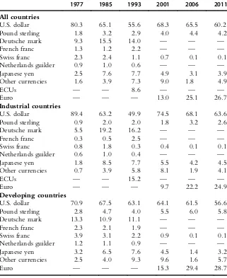
The foreign exchange market is the largest financial market in the world. In April 2010, the Bank for International Settlements (BIS) conducted a survey of trading volume around the world and found that the average amount of currency traded each business day was $3,981 billion. In 2001 the trading volume of foreign exchange was $1,239 billion. Thus, the amount of foreign exchange traded has recently grown tremendously. The U.S. dollar is by far the most important currency, and has remained so in the last decade, even with the introduction of the euro. The dollar is involved in 85 percent of all trades. Since foreign exchange trading involves pairs of currencies, it is useful to know which currency pairs dominate the market.
Table 1.1 reports the share of market activity taken by different cur-rencies. The largest volume occurs in dollar/euro trading, accounting for almost 30 percent of the total. The next closest currency pair, the dollar/ yen, involves roughly half as much spot trading as the dollar/euro. After these two currency pairs, the volume drops off dramatically. Thus, the currency markets are dominated by dollar trading.
3 International Money and Finance, Eighth Edition
DOI:http://dx.doi.org/10.1016/B978-0-12-385247-2.00001-9
GEOGRAPHIC FOREIGN EXCHANGE RATE ACTIVITY
The foreign exchange market is a 24-hour market. Currencies are quoted continuously across the world. Figure 1.1 illustrates the 24-hour dimen-sion of the foreign exchange market. We can determine the local hours of major trading activity in each location by the country bars at the top of the figure. Time is measured as Greenwich Mean Time (GMT) at the bottom of the figure. For instance, in New York 7 A.M. is 1200 GMT and 3 P.M. is 2000 GMT. Since London trading has ended by 4 P.M. London time, or 1600 GMT (11 A.M. in New York), active arbitrage involving comparisons of New York and London exchange rate quotes would end around 1600 GMT. Figure 1.1 shows that there is a small overlap between European trading and Asian trading, and there is no overlap between New York trading and Asian trading.
Dealers in foreign exchange publicize their willingness to deal at certain prices by posting quotes on news services such as Reuters. When a dealer at a bank posts a quote on a news service, that quote then appears on com-puter monitors sitting on the desks of other foreign exchange market parti-cipants worldwide. This posted quote is like an advertisement, telling the rest of the market the prices at which the quoting dealer is ready to deal.
The actual prices at which transactions are carried out will have nar-rower spreads than the bid and offer prices quoted on the news service screens. These transaction prices are proprietary information and are known only by the two participants in a transaction. The quotes on the
Table 1.1 Top Ten Currency Pairs by Share of Foreign Exchange Trading Volume
Currency pair Percent of total
U.S. dollar/euro 28
U.S. dollar/Japanese yen 14
U.S. dollar/U.K. pound 9
U.S. dollar/Australian dollar 6 U.S. dollar/Canadian Dollar 5 U.S. dollar/Swiss franc 4
Euro/Japanese yen 3
Euro/U.K. pound 3
Euro/Swiss franc 2
U.S. dollar/Swedish krona 1
Source:Table created from data found in Bank for International Settlements, Triennial Central Bank Survey; Report on Global Foreign Exchange Market Activity in 2010,Basel, December, 2010.
news service screens are the best publiclyavailable information on the cur-rent prices in the market.
In terms of the geographic pattern of foreign exchange trading, a small number of locations account for the majority of trading.Table 1.2reports the average daily volume of foreign exchange trading in different countries. The United Kingdom and the United States account for half of total world ing. The United Kingdom has long been the leader in foreign exchange trad-ing. In 2010, it accounted for 37 percent of total world trading volume. While it is true that foreign exchange trading is a round-the-clock business, with trading taking place somewhere in the world at any point in time, the peak activity occurs during business hours in London, New York, and Tokyo.
more than 20 quotes per hour being entered on the Reuters screen. Quoting activity rises and falls through the Asian morning until reaching a daily low at lunch time in Tokyo (0230 0330 GMT).
Table 1.2 Top Ten Foreign Exchange Markets by Trading Volume (daily averages)
Country Total volume (billions of dollars)
Percent share
United Kingdom 1,854 37
United States 904 18
Japan 312 6
Singapore 266 5
Switzerland 263 5
Hong Kong 238 5
Australia 192 4
France 152 3
Denmark 120 2
Germany 109 2
Source:Table created from data found in Bank for International Settlements, Triennial Central Bank Survey; Report on Global Foreign Exchange Market Activity in 2010,Basel, December 2010.
Hours are Greenwich Mean Time Monday
0 0 1 2 3 4 5 6 7 8 910 11 12 13 14 15 16 17 18 19 20 21 22 23 0 1 2 3 4 5 6 7 8 910 11 12 13 14 15 16 17 18 19 20 21 22 23 0 1 2 3 4 5 6 7 8 910 11 12 13 14 15 16 17 18 19 20 21 22 23 0 1 2 3 4 5 6 7 8 910 11 12 13 14 15 16 17 18 19 20 21 22 23 0 1 2 3 4 5 6 7 8 910 11 12 13 14 15 16 17 18 19 20 21 22 23
20
Quotes per hour
40 60 80 100 120 140 160
Tuesday Wednesday Thursday Friday
Figure 1.2 Average hourly weekday quotes, Japanese yen per U.S. dollar.
The lull in trading during the Tokyo lunch hour was initially the result of a Japanese regulation prohibiting trading during this time. Since December 22, 1994, trading has been permitted in Tokyo during lunch-time, but there still is a pronounced drop in activity because many traders take a lunch break. Following the Tokyo lunch break, market activity picks up in the Asian afternoon and rises substantially as European trading begins around 0700 GMT. There is another decrease in trading activity associated with lunchtime in Europe, 1200 to 1300 GMT. Trading rises again when North American trading begins, around 1300 GMT, and hits a daily peak when London and New York trading overlap. Trading drops substantially with the close of European trading, and then rises again with the opening of Asian trading the next day.
Note that every weekday has this same pattern, as the pace of the activity in the foreign exchange market follows the opening and closing of business hours around the world. While it is true that the foreign exchange market is a 24-hour market with continuous trading possible, the amount of trading follows predictable patterns. This is not to say that there are not days that differ substantially from this average daily number of quotes. If some surprising event occurs that stimulates trading, some days may have a much different pattern. Later in the text we consider the determinants of exchange rates and study what sorts of news would be especially relevant to the foreign exchange market.
SPOT EXCHANGE RATES
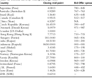
A spot exchange rate is the price of one money in terms of another that is delivered today. Table 1.3 shows spot foreign exchange rate quotations for a particular day. In the table we see that on Tuesday, April 26, 2011, the U.S. dollar sold for 0.8795 Swiss francs. Note that this exchange rate is quoted at a specific time, 4 P.M. Greenwich Mean Time, since rates will change throughout the day as supply and demand for the currencies change. Notice also that these exchange rates are quotes based on large trades ($1 million or more), in what is essentially a wholesale market. For instance, if you were a U.S. importer buying watches from Switzerland at the dollar price of $10 million, a bank would sell $10 million worth of Swiss francs to you for 0.8795 Swiss franc per dollar. You would receive SF 8.795 million to settle the account with the Swiss exporter.
If the amount traded was less than $1 million the cost of foreign exchange would be higher. The smaller the quantity of foreign exchange purchased, the higher the price. Therefore if you travel to a foreign coun-try the exchange rate will be much less favorable for you as a tourist.
In the previous example, the U.S. importer found that $10 million was equivalent in value to SF8.795 million. We calculated this by multi-plying the total dollar value of the purchase by the Swiss franc price of a dollar price. If we need to convert Swiss francs into dollars, then we will divide the Swiss franc amount by the exchange rate, or multiply the Swiss franc amount by the reciprocal of the exchange rate. If a U.S. man-ufacturer is exporting cars to Switzerland and receives SF12 million then Table 1.3 Selected Currency Trading Exchange Rates
Country Closing mid-point Bid-Offer spread
Argentina (Peso) 4.0813 780 845
Australia (Australian $) 0.9289 767 763
Brazil (Real) 1.5640 635 645
Canada (Canadian $) 0.9515 512 517
China (Yuan) 6.5287 NA
Czech Republic (Koruna) 16.4519 390 647
Denmark (Danish Krone) 5.0979 971 987
Ecuador (US Dollar) 1.0000
Hong Kong (Hong Kong $) 7.7713 710 715
Hungary (Forint) 181.0440 065 816
India (Rupee) 44.5150 100 200
Indonesia (Rupiah) 8650.0000 000 000
Israel (Shekel) 3.4185 175 195
Japan (Yen) 81.7050 690 720
Norway (Norwegian Krone) 5.3196 175 217
Russia (Rouble) 27.7950 800 100
Sweden (Krona) 6.0988 969 007
Switzerland (Franc) 0.8795 792 798
U.K. (Pound) 1.6450 448 452
Euro (Euro) 1.4626 624 628
SDR (SDR) 0.6214
The London foreign exchange mid-range rates above apply to trading among banks in amounts of $1 million and more, as quoted at 4 P.M. GMT by Reuters. The quotes are in foreign currency per dollar, except for the U.K. pound and the euro that are quoted as dollar per foreign currency. Source:Table is based on data fromFinancial Times, Currency Markets: Dollar Spot Forward against the Dollar and Dollar against Other Currencies on April 26, 2011.
See:http://markets.ft.com/RESEARCH/markets
we divide by the exchange rate SF12/0.87955$13.644 million. We could also have multiplied the SF12 by the reciprocal 1/0.879551.137 to reach the same amount. It will always be true that when we know the dollar price of the franc ($/SF), we can find the Swiss franc price of the dollar by taking the reciprocal 1/($/SF)5(SF/$).
Note that the exchange rate quotes in the first column in Table 1.3
are mid-range rates. Banks buy (bid) foreign exchange at lower rates than they sell (offer), and the difference between the selling and buying rates is called the spread. The mid-range is the average of the buying and selling rates. Table 1.3 lists the spreads for each currency in the second column. The bid/offer spread is quoted so that one can see the bid(buy) price by dropping the last three digits and replacing them with the first number. Similarly, the offer(sell) price is found by dropping the last three digits of the mid-point quote and replacing them with the second number. For example, the Swiss franc bid offer spread is 0.8792 0.8798. Thus, the bank is willing to buy dollars for Swiss francs at 0.8792, and sell dollars at 0.8798 Swiss francs. This spread of less than 1/100 of 1 percent [(0.879820.8792)/0.87925 .000068] is indicative of how small the normal spread is in the market for major traded currencies. The existing spread in any currency will vary according to the individual currency trader, the currency being traded, and the trading bank’s overall view of conditions in the foreign exchange market. The spread quoted will tend to increase for more thinly traded currencies (i.e., currencies that do not generate a large volume of trading) or when the bank perceives that the risks associated with trading in a currency at a particular time are rising.
The large trading banks like Citibank or Deutsche Bank stand ready to “make a market” in a currency by offering buy (bid) and sell (offer) rates on request. Actually, currency traders do not quote all the numbers indicated in Table 1.3. For instance, the table lists the spread on euro as 624 628. In practice, this spread is quoted as $1.4624 28 or, in words, the U.S. dollar per euro rate is one-forty-six-twenty-four to twenty-eight. The listener then recognizes that the bank is willing to bid $1.4624 to buy one euro and will sell euros at $1.4628.
trading at an official exchange rate, regardless of current market conditions.
This chapter discusses the buying and selling of foreign exchange to be delivered on the spot (actually, deposits traded in the foreign exchange market generally take two working days to clear); this is called thespot mar-ket.In Chapter 4 we will consider the important issues that arise when the trade contract involves payment at a future date. First, however, we should consider in more detail the nature of the foreign exchange market.
CURRENCY ARBITRAGE
The foreign exchange market is a market where price information is readily available by telephone or computer network. Since currencies are
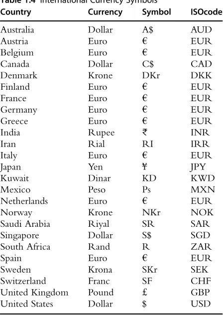
Table 1.4 International Currency Symbols
Country Currency Symbol ISOcode
Australia Dollar A$ AUD
Austria Euro h EUR
Belgium Euro h EUR
Canada Dollar C$ CAD
Denmark Krone DKr DKK
Finland Euro h EUR
France Euro h EUR
Germany Euro h EUR
Greece Euro h EUR
India Rupee R INR
Iran Rial RI IRR
Italy Euro h EUR
Japan Yen f JPY
Kuwait Dinar KD KWD
Mexico Peso Ps MXN
Netherlands Euro h EUR
Norway Krone NKr NOK
Saudi Arabia Riyal SR SAR
Singapore Dollar S$ SGD
South Africa Rand R ZAR
Spain Euro h EUR
Sweden Krona SKr SEK
Switzerland Franc SF CHF
United Kingdom Pound d GBP
United States Dollar $ USD
homogeneous goods (a dollar is a dollar regardless of where it is traded), it is very easy to compare prices in different markets. Exchange rates tend to be equal worldwide. If this were not so, there would be profit oppor-tunities for simultaneously buying a currency in one market while selling it in another. This activity, known as arbitrage, would raise the exchange rate in the market where it is too low, because this is the market in which you would buy, and the increased demand for the currency would result in a higher price. The market where the exchange rate is too high is one in which you sell, and this increased selling activity would result in a lower price. Arbitrage would continue until the exchange rates in differ-ent locales are so close that it is not worth the costs incurred to do any further buying and selling. When this situation occurs, we say that the rates are “transaction costs close.” Any remaining deviation between exchange rates will not cover the costs of additional arbitrage transactions, so the arbitrage activity ends.
For instance, suppose the following quotes were available for the Swiss franc/U.S. dollar rate:
• Citibank is quoting 0.8745 55
• Deutsche Bank in Frankfurt is quoting 0.8725 35
This means that Citibank will buy dollars for 0.8745 francs and will sell dollars for 0.8755 francs. Deutsche Bank will buy dollars for 0.8725 francs and will sell dollars for 0.8735 francs. This presents an arbitrage opportunity. We call this a two-point arbitrageas it involves two currencies. We could buy $10 million at Deutsche Bank’s offer price of 0.8735 and simultaneously sell $10 million to Citibank at their bid price of 0.8745 francs. This would earn a profit of SF0.0010 per dollar traded, or SF10,000 would be the total arbitrage profit.
spreads of SF0.001. In the wholesale banking foreign exchange market, the bid offer spread is the only transaction cost. When the quotes of two different banks differ by no more than the spread being quoted in the market by these banks, there is no arbitrage opportunity.
Arbitrage could involve more than two currencies. Since banks quote foreign exchange rates with respect to the dollar, one can use the dollar value of two currencies to calculate thecross ratebetween the two curren-cies. The cross rate is the implied exchange rate from the two actual quotes. For instance, if we know the dollar price of pounds ($/d) and the dollar price of Swiss francs ($/SF), we can infer what the corresponding pound price of francs (d/SF) would be. From now on we will explicitly write the units of our exchange rates to avoid the confusion that can eas-ily arise. For example, $/d5$1.76 is the exchange rate in terms of dollars per pound.
Suppose that in London $/d5$1.76, while in New York $/SF5 $1.10. The correspondingcross rateis the d/SF rate. Simple algebra shows that if $/d5$1.76 and $/SF51.1, then d/SF5($/SF)/($/d), or 1.10/ 1.7650.625. If we observe a market where one of the three exchange rates—$/d, $/SF, d/SF—is out of line with the other two, there is an arbitrage opportunity, in this case atriangular arbitrage. Triangular arbitrage, orthree-point arbitrage, involves three currencies.
To simplify the analysis of arbitrage involving three currencies, let us temporarily ignore the bid offer spread and assume that we can either buy or sell at one price. Suppose that in Geneva, Switzerland the exchange rate is d/SF50.625, while in New York $/SF51.100, and in London $/d5$1.600.
Table 1.5appears to have no possible arbitrage opportunity, but astute traders in the foreign exchange market would observe a discrepancy when they check the cross rates. Computing the implicit cross rate for New York, the arbitrageur finds the implicit cross rate to be d/SF5 ($/SF)/($/d), or 1.100/1.60050.6875. Thus the cost of SF is high in New York, and the cost ofdis low.
Table 1.5 Triangular Arbitrage
Location $/SF $/d d/SF
New York 1.100 1.600
London 1.600 0.625
Geneva 1.100 0.625
Assume that a trader starts in New York with 1 million dollars. The trader should buy d in New York. Selling $1 million in New York (or London) the trader receives d625,000 ($1 million divided by $/d 5
$1.60). The pounds then are used to buy Swiss francs at d/SF 5 0.625 (in either London or Geneva), so thatd625,000 5SF1 million. The SF1 million would be used in New York to buy dollars at $/SF 5 $1.10, so that SF1 million 5 $1,100,000. Thus the initial $1 million could be turned into $1,100,000, with the triangular arbitrage action earning the trader $100,000 (costs associated with the transaction should be deducted to arrive at the true arbitrage profit).
As in the case of the two-currency arbitrage covered earlier, a valuable product of this arbitrage activity is the return of the exchange rates to internationally consistent levels. If the initial discrepancy was that the dol-lar price of pounds was too low in London, the selling of doldol-lars for pounds in London by the arbitrageurs will make pounds more expensive, raising the price from $/d 5 $1.60. Note that if the pound cost increases to $/d 5 $1.76 then there is no arbitrage possible. However, the pound exchange rate is unlikely to increase that much because the activity in the other markets would tend to raise the pound price of francs and lower the dollar price of francs, so that a dollar price of pounds somewhere between $1.60 and $1.76 would be the new equilibrium among the three currencies.
Since there is active trading between the dollar and other currencies, we can look to any two exchange rates involving dollars to infer the cross rates. So even if there is limited direct trading between, for instance, Mexican pesos and yen, by using pesos/$ and $/f, we can find the implied pesos/f rate. Since transaction costs are higher for lightly traded currencies, the depth of foreign exchange trading that involves dollars often makes it cheaper to go through dollars to get from some currency X to another currencyY when Xand Yare not widely traded. Thus, if a business firm in small countryXwants to buy currency Yto pay for mer-chandise imports from small country Y, it may well be cheaper to sell X for dollars and then use dollars to buy Yrather than try to trade currency Xfor currency Ydirectly.
SHORT-TERM FOREIGN EXCHANGE RATE MOVEMENTS
foreign exchange traders adjust their bid and offer quotes throughout the business day.
A foreign exchange trader may be motivated to alter his or her exchange rate quotes in response to changes in his or her position with respect to orders to buy and sell a currency. For instance, suppose Helmut Smith is a foreign exchange trader at Deutsche Bank, who specializes in the dollar/euro market. The bank management controls risks associated with foreign currency trading by limiting the extent to which traders can take a position that would expose the bank to potential loss from unex-pected changes in exchange rates. If Smith has agreed to buy more euros than he has agreed to sell, he has along positionin the euro and will profit from euro appreciation and lose from euro depreciation. If Smith has agreed to sell more euros than he has agreed to buy, he has ashort position in the euro and will profit from euro depreciation and lose from euro appreciation. His position at any point in time may be called hisinventory. One reason traders adjust their quotes is in response to inventory changes. At the end of the day most traders balance their position and are said to go home “flat.” This means that their orders to buy a currency are just equal to their orders to sell. Thus, the profit the bank receives is from trading activity, not from speculative activity.
FAQ: What Is a Rogue Trader?
Many bank traders are required to balance their positions daily. This is done to eliminate the risk that the overnight position changes in value dramati-cally. Note that in the arbitrage case the buying and selling is almost instan-taneous. Therefore, there is practically no risk. The longer one has to wait for an offsetting position, the more risk there is. Thus, there is a speculative risk when a bank adopts a one-sided bet. An overnight position would be too much risk for most banks to accept, as this is a high-risk speculation.
However, banks have been subject to fraud at times where they seem to be unable to control what traders do. If traders take on their own bets in exception to the bank’s risk controls then they have become“rogue traders.” In September 2011, UBS bank discovered that one of their traders, Kweku Adoboli, had entered into upwards of $10 billion in trades with fictitious off-set trades. Effectively this created risky positions that lost UBS as much as $2.3 billion.
The most famous “rogue trader” is Nick Leeson, who lost $1.3 billion while working for Barings Investment bank in the early 1990s. He bought futures contracts without any offsetting transactions, claiming that they were purchase orders on behalf of a client. The loss to Barings Investment bank
was so high that the well-respected bank that had existed over 200 years had to declare bankruptcy. Nick received a prison sentence in a Singapore jail for six and half years. For more on the life of Nick Leeson, see Leeson (2011) or watch Ewan McGregor starring as Nick Leeson in the movieRogue Trader.
Let us look at an example. Suppose Helmut Smith has been buying and selling euros for dollars throughout the day. By early afternoon his position is as follows:
dollar purchases: $100,000,000 dollar sales: $80,000,000
In order to balance his position, Smith will adjust his quotes to encourage fewer dollar purchases and more dollar sales. For instance, if the euro is currently trading at $1.4650 60, then Helmut could raise the bid and offer quotes to encourage others to sell him euros in exchange for his dollars, while deterring others from buying more euros from him. For instance, if he changes the quote to 1.4655 65, then someone could sell him euros (or buy his dollars) for $1.4655 per euro. Since he has raised the dollar price of a euro, he will receive more interest from people wanting to sell him euros in exchange for his dollars. When Helmut buys euros from other traders, he is selling them dollars, and this helps to bal-ance his inventory and reduce his long position in the dollar. At the same time Helmut has raised the sell rate of euros to $1.4665. This discourages other traders from buying more euros from Helmut (giving him dollars as payments).
This inventory control effect on exchange rates can explain why tra-ders may alter their quotes in the absence of any news about exchange rate fundamentals. Evans and Lyons (2002) studied the German mark/ dollar market before there was a euro and estimated that, on average, foreign exchange traders alter their quotes by .00008 for each $10 mil-lion of undesired inventory. So a trader with an undesired long mark position of $20 million would, on average, raise his quote by .00016.
1.0250 60 and is called by Ingrid Schultz at Citibank asking to buy $5 million of euros at Helmut’s offer price of 1.0260, Helmut then must wonder whether Ingrid knows something he doesn’t. Should Ingrid’s order to trade at Helmut’s price be considered a signal that Helmut’s price is too low? What superior information could Ingrid have? Every bank receives orders from nonbank customers to buy and sell currency. Perhaps Ingrid knows that her bank has just received a large order from Daimler Benz to sell dollars, and she is selling dollars (and buying euros) in advance of the price increase that will be caused by this nonbank order being filled by purchasing euros from other traders.
Helmut does not know why Ingrid is buying euros at his offer price, but he protects himself from further euro sales to someone who may be better informed than he is by raising his offer price. The bid price may be left unchanged because the order was to buy his euros; in such a case the spread increases, with the higher offer price due to the possibility of trading with a better-informed counterparty. Lyons (1995) estimated that the presence of asymmetric information among traders resulted in the average change in the quoted price being .00014 per $10 million traded. At this average level, Helmut would raise his offer price by .00007 in response to Ingrid’s order to buy $5 million.
The inventory control and asymmetric information effects can help explain why exchange rates change throughout the day, even in the absence of news regarding the fundamental determinants of exchange rates. The act of trading generates price changes among risk-averse traders who seek to manage their inventory positions to limit their exposure to surprising exchange rate changes and limit the potential loss from trading with better-informed individuals.
LONG-TERM FOREIGN EXCHANGE MOVEMENTS
Thus far we have examined short-run movements in exchange rates. For the most part we are interested in long-term movements in this book. Since the exchange rate is the price of one money in terms of another, changes in exchange rates affect the prices of goods and services traded internationally. Therefore most of this book is concerned with why exchange rates move and how we can avoid these effects. In this section we will introduce a simple but powerful tool, called the trade flow model. The trade flow model argues that the exchange rate responds to the demand for traded goods by countries.
We can use a familiar diagram from principles of economics courses— the supply and demand diagram. Figure 1.3 illustrates the market for the yen/dollar exchange rate. Think of the demand for dollars as coming from the Japanese demand for U.S. goods (they must buy dollars in order to purchase U.S. goods). The downward-sloping demand curve illustrates that the higher the yen price of the dollar, the more expensive U.S. goods are to Japanese buyers, so the smaller the quantity of dollars demanded. The supply curve is the supply of dollars to the yen/dollar market and comes from U.S. buyers of Japanese goods (in order to obtain Japanese products, U.S. importers have to supply dollars to obtain yen). The upward-sloping supply curve indicates that as U.S. residents receive more yen per dollar, they will buy more from Japan and will supply a larger quantity of dollars to the market.
The initial equilibrium exchange rate is at point A, where the exchange rate is 90 yen per dollar. Now suppose there is an increase in Japanese demand for U.S. products. This increases the demand for dollars so that the demand curve shifts from D1 to D2. The equilibrium exchange rate will now change to 100 yen per dollar at point B as the dollar appreciates in value against the yen. This dollar appreciation makes Japanese goods cheaper to U.S. buyers.
In the above example the demand for U.S. dollars changed. The sup-ply may also change. Such an example is illustrated in Figure 1.4. Assume that the U.S. starts at point B with a 100 yen/$ exchange rate. If U.S. consumers start liking Japanese products more than before, this will result in a supply curve shift. U.S. importers will be more eager to give up their
A B
S
100
90
0
Quantity of dollars D1
D2
Y
en/dollar e
xchange r
ate
dollars in exchange for yen. This shifts the supply curve out to the right, from S1 to S2, and lowers the value of the dollar. The new equilibrium is at point C, where the yen/dollar rate is at 85.
100
85
0
Y
en/dollar e
xchange r
ate
Quantity of dollars D
C B
S1
S2
Figure 1.4 Traders’increased supply of dollars decreases the dollar value.
The examples above illustrate that the trade flow model can be a use-ful model to show the exchange rate changes in response to changes in demand for products in two countries. In the next chapter we will expand the trade flow model by adding central bank intervention. Later in the text we will examine other models that can explain exchange rate movements.
SUMMARY
1. The foreign exchange market is a global market where foreign cur-rency deposits are traded. Trading in actual curcur-rency notes is generally limited to tourism or illegal activities.
2. The dollar/euro currency pair dominates foreign exchange trading volume, and the United Kingdom is the largest trading location. 3. A spot exchange rate is the price of a currency in terms of another
currency for current delivery. Banks buy (bid) foreign exchange at a lower rate than they sell (offer), and the difference between the selling and buying rates is called the spread.
4. Arbitrage realizes riskless profit from market disequilibrium by buying a currency in one market and selling it in another. Arbitrage ensures that exchange rates are transaction costs close in all markets.
5. The factors that explain why exchange rates vary so much in the short run are inventory control and asymmetric information.
6. In the long run, economic factors (e.g., demand/supply of foreign and domestic goods) affect the exchange rate movements. The trade flow model is useful for discussing fundamental changes in the foreign exchange rate.
EXERCISES
1. Suppose f15$0.0077 in London, $15SF2.00 in New York, and SF15 f65 in Paris.
a. If you begin by holding 10,000 yen, how could you make a profit from these exchange rates?
b. Find the arbitrage profit per yen initially traded. (Ignore transac-tion costs.)
2. Suppose Sumitomo Bank quotes thef/$ exchange rate as 110.30 .40 and Nomura Bank quotes 110.40 .50. Is there an arbitrage opportu-nity? If so, explain how you would profit from these quotes. If not, explain why not.
3. What is the cross rate implied by the following quotes? a. C$/$51.5613, $/h51.0008
b. f/$5124.84, $/d51.5720 c. SF/$51.4706, C$/$5 1.5613
4. Suppose that the spot rates of the U.S. dollar, British pound, and Swedish kronor are quoted in three locations as the following:
$/d $/SKr SKr/d New York 2.00 0.25 –
London 2.00 – 10.00
Stockholm – 0.25 10.00
Is there an arbitrage opportunity? If so, explain how you, as a trader who has $1,000,000, would profit from these quotes. If not, explain why not.
FURTHER READING
Bank for International Settlements, Triennial Central Bank Survey; Report on Global
Foreign Exchange Market Activity in 2010, Basel, December, 2010.
Berger, D.W., Chaboud, A.P., Chernenko, S.V., Howorka, E., Wright, J., 2008. Order flow and exchange rate dynamics in electronic brokerage system data. J. Int. Econ. 75 (1), 93 109.
Evans, M., Lyons, R., 2002. Order flow and exchange rate dynamics. J. Polit. Econ. Vol. 110 (No. 1), 170 180.
The Foreign Exchange Market in the United States, Federal Reserve Bank of New York,
,http://www.newyorkfed.org/education/addpub/usfxm/..
Leeson, Nick, 2011.,www.nickleeson.com..
Lyons, R.K., 1995. Tests of microstructural hypotheses in the foreign exchange market. J. Financ. Econ. 39, 321 351.
Norrbin, S., Pipatchaipoom, O., 2007. Is the real dollar rate highly volatile? Econ. Bull. Vol. 6 (No. 2), 1 15.
APPENDIX 1A: TRADE-WEIGHTED EXCHANGE RATE INDEXES
Suppose we want to consider the value of a currency. One measure is the bilateral exchange rate—say, the yen value of the dollar. However, if we are interested in knowing how a currency is performing globally, we need a broader measure of the currency’s value against many other currencies. This is analogous to looking at a consumer price index to measure how prices in an economy are changing. We could look at the price of shoes or the price of a loaf of bread, but such single-good prices will not necessarily reflect the gen-eral inflationary situation—some prices may be rising while others are falling.
In the foreign exchange market it is common to see a currency rising in value against one foreign money while it depreciates relative to another. As a result, exchange rate indexes are constructed to measure the average value of a currency relative to several other currencies. An exchange rate index is a weighted average of a currency’s value relative to other currencies, with the weights typically based on the importance of each currency to international trade. If we want to construct an exchange rate index for the United States, we would include the currencies of the countries that are the major trading partners of the United States.
If half of U.S. trade was with Canada and the other half was with Mexico, then the percentage change in the trade-weighted dollar exchange rate index would be found by multiplying the percentage change in both the Canadian dollar/U.S. dollar exchange rate and the Mexican peso/U.S. dollar exchange rate by one-half and summing the result.
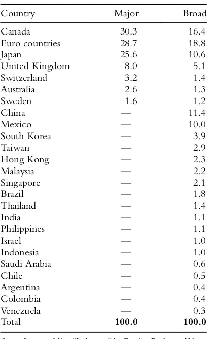
Table 1A.1 lists two popular exchange rate indexes and their weighting
schemes. The indexes listed are the Federal Reserve Board’sMajor Currency Index, (TWEXMMTH) and theBroad Currency Index(TWEXBMTH).
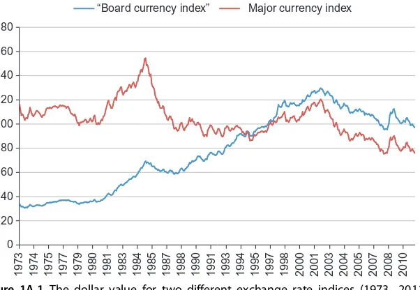
Since the different indexes are constructed using different currencies, should we expect them to tell a different story? It is entirely possible for a currency to be appreciating against some currencies while it depreciates against others. Therefore, the exchange rate indexes will not all move identically. Figure 1A.1 plots the movement of the various indexes over time.
Table 1A.1 Percentage Weights Assigned to Major Currencies in Two U.S. Dollar Exchange Rate Indexes
Exchange rate index
Country Major Broad
Canada 30.3 16.4
Euro countries 28.7 18.8
Japan 25.6 10.6
United Kingdom 8.0 5.1
Switzerland 3.2 1.4
Australia 2.6 1.3
Sweden 1.6 1.2
China — 11.4
Mexico — 10.0
South Korea — 3.9
Taiwan — 2.9
Hong Kong — 2.3
Malaysia — 2.2
Singapore — 2.1
Brazil — 1.8
Thailand — 1.4
India — 1.1
Philippines — 1.1
Israel — 1.0
Indonesia — 1.0
Saudi Arabia — 0.6
Chile — 0.5
Argentina — 0.4
Colombia — 0.4
Venezuela — 0.3
Total 100.0 100.0
Figure 1A.1indicates that the value of the dollar generally rose in the early 1980s—a conclusion we draw regardless of the exchange rate index used. Differences arise in the 1990s where the dollar stayed fairly constant against the major currencies, but appreciated according to the broad cur-rency index. In the 2000s both indexes again tell the same story, with both indexes showing a depreciating dollar. Since different indexes assign a different importance to each foreign currency, this is not surprising. For instance, if we look at the weights inTable 1A.1, then a period in which the dollar appreciated rapidly against the Mexican peso relative to other currencies would result in the Major Currency Index to record a smaller dollar appreciation relative to the Broad Currency Index. This is because the peso accounts for 10 percent of the Broad Currency Index, but zero for the Major Currency Index.
Exchange rate indexes are commonly used analytical tools in interna-tional economics. When changes in the average value of a currency are important, bilateral exchange rates (between only two currencies) are unsatisfactory. Neither economic theory nor practice gives a clear indica-tion of which exchange rate index is best. In fact, for some quesindica-tions there is little to differentiate one index from another. In many cases, how-ever, the best index to use will depend on the question addressed.
180
“Board currency index” Major currency index
160
140
120
100
80
60
40
20
0
1973 1974 1975 1977 1979 1980 1981 1983 1984 1985 1987 1988 1990 1991 1993 1994 1995 1997 1998 2000 2001 2003 2004 2005 2007 2008 2010 Figure 1A.1 The dollar value for two different exchange rate indices (1973 2011).
Source: Federal Reserve Bank of St. Louis, FRED data, Authors’calculation.
APPENDIX 1B: THE TOP FOREIGN EXCHANGE DEALERS
Foreign exchange trading is dominated by large commercial banks with worldwide operations. The market is very competitive, since each bank tries to maintain its share of the corporate business. Euromoney magazine provides some interesting insights into this market by publishing periodic surveys of information supplied by the treasurers of the major multina-tional firms.
When asked to rank the factors that determined who got their foreign exchange business, the treasurers responded that the following factors were the most important: The speed with which a bank makes foreign exchange quotes was ranked third. A second-place ranking was given to competitiveness of quotes. The most important factor was the firm’s rela-tionship with the bank. A bank that handles the other banking needs of a firm is also likely to receive its foreign exchange business.
The significance of competitive quotes is indicated by the fact that treasurers often contact more than one bank to get several quotes before placing a deal. Another implication is that the market will be dominated by the big banks, because only the giants have the global activity to allow competitive quotes on a large number of currencies. Table 1B.1gives the rankings of the Euromoney survey. According to the rankings, Deutsche Bank receives more business than any other bank. Note also that the big
Table 1B.1 The Top 15 Foreign Exchange Dealers with Market Share
1. Deutsche Bank (18.1%) 2. UBS (11.3%)
3. Barclays Capital (11.1%) 4. Citi (7.7%)
5. Royal Bank of Scotland (6.5%) 6. JPMorgan (6.4%)
7. HSBC (4.6%) 8. Credit Suisse (4.4%) 9. Goldman Sachs (4.3%) 10. Morgan Stanley (2.9%) 11. BNP Paribas (2.9%)
12. Bank of America Merrill Lynch (2.3%) 13. Societe Generale (2.1%)
14. Commerzbank (1.5%) 15. Standard Chartered (1.2%)
three—Deutsche Bank, UBS and Barclays Capital—dominate the foreign exchange market
What makes Deutsche Bank the world’s best foreign exchange dealer? Many factors have kept them on top of the heap. An important factor is simply sheer size. Deutsche Bank holds the bank accounts for many corporations, giving it a natural advantage in foreign exchange trading. Foreign exchange trading has emerged as an important center for bank profitability. Since each trade generates revenue for the bank, the volatile foreign exchange markets of recent years have often led to frenetic activity in the market with a commensurate revenue increase for the banks.
CHAPTER
2
2
International Monetary
Arrangements
Like most areas of public policy, international monetary relations are sub-ject to frequent proposals for change. Fixed exchange rates, floating exchange rates, and commodity-backed currency all have their advocates. Before considering the merits of alternative international monetary sys-tems, we should understand the background of the international mone-tary system. Although an international monemone-tary system has existed since monies have been traded, it is common for most modern discussions of international monetary history to start in the late nineteenth century. It was during this period that the gold standard began.
THE GOLD STANDARD: 1880 TO 1914
Although an exact date for the beginning of the gold standard cannot be pinpointed, we know that it started during the period from 1880 to 1890. Under a gold standard, currencies are valued in terms of their gold equivalent (an ounce of gold was worth $20.67 in terms of the U.S. dollar over the gold standard period). The gold standard is an important begin-ning for a discussion of international monetary systems because when each currency is defined in terms of its gold value, all currencies are linked in a system of fixed exchange rates. For instance, if currency A is worth 0.10 ounce of gold, whereas currency B is worth 0.20 ounce of gold, then 1 unit of currency B is worth twice as much as 1 unit of A, and thus the exchange rate of 1 currencyB52 currencyA is established.
Maintaining a gold standard requires a commitment from participating countries to be willing to buy and sell gold to anyone at the fixed price. To maintain a price of $20.67 per ounce, the United States had to buy and sell gold at that price. Gold was used as the monetary standard because it is a homogeneous commodity (could you have a fish standard?) worldwide that is easily storable, portable, and divisible into standardized units like ounces. Since gold is costly to produce, it possesses another
25 International Money and Finance, Eighth Edition
DOI:http://dx.doi.org/10.1016/B978-0-12-385247-2.00002-0
important attribute—governments cannot easily increase its supply. A gold standard is a commodity money standard. Money has a value that is fixed in terms of the commodity gold.
One aspect of a money standard that is based on a commodity with relatively fixed supply is long-run price stability. Since governments must maintain a fixed value of their money relative to gold, the supply of money is restricted by the supply of gold. Prices may still rise and fall with swings in gold output and economic growth, but the tendency is to return to a long-run stable level.Figure 2.1illustrates graphically the rela-tive stability of U.S. and U.K. prices over the gold standard period as compared to later years. However, note also that prices fluctuated up and down in the short run during the gold standard. Thus, frequent small bursts of inflation and deflation occurred in the short run, but in the long run the price level remained unaffected. Since currencies were convert-ible into gold, national money supplies were constrained by the growth of the stock of gold. As long as the gold stock grew at a steady rate, prices would also follow a steady path. New discoveries of gold would generate discontinuous jumps in the price level, but the period of the gold stan-dard was marked by a fairly stable stock of gold.
People today often look back on the gold standard as a “golden era” of economic progress. It is common to hear arguments supporting a
420
End of gold standard End of gold standard
1940 1960 1980 1880
Figure 2.1 U.S. and U.K. wholesale price indexes from 1880 to 1976. Data are missing for World War II years in the United Kingdom. Source: Roy W. Jastram,The Golden Constant, New York: Wiley, 1977.
return to the gold standard. Such arguments usually cite the stable prices, economic growth, and development of world trade during this period as evidence of the benefits provided by such an orderly international mone-tary system. Others have suggested that the economic development and stability of the world economy in those years did not necessarily reflect the existence of the gold standard but, instead, the absence of any signifi-cant real shocks such as war. Although we may disagree on the merits of returning to a gold standard, it seems fair to say that the development of world trade was encouraged by the systematic linking of national curren-cies and the price stability of the system. Since gold is like a world money during a gold standard, we can easily understand how a balance of pay-ments disequilibrium may be remedied. A country running a balance of payments (official settlements) deficit would find itself with net outflows of gold, which would reduce its money supply and, in turn, its prices. A surplus country would find gold flowing in and expanding its money supply, so that prices rose. The fall in price in the deficit country would lead to greater net exports (exports minus imports), and the rise in price in the surplus country would reduce its net exports, so that balance of payments equilibrium would be restored.
In practice, actual flows of gold were not the only, or even necessarily the most important, means of settling international debts during this period. Since London was the financial center of the world, and England the world’s leading trader and source of financial capital, the pound also served as a world money. International trade was commonly priced in pounds, and trade that never passed through England was often paid for with pounds.
THE INTERWAR PERIOD: 1918 TO 1939