Boston Burr Ridge, IL Dubuque, IA Madison, WI New York San Francisco St. Louis Bangkok Bogotá Caracas Lisbon London Madrid
Mexico City Milan New Delhi Seoul Singapore Sydney Taipei Toronto
C
Ch
Modern Analytical Chemistry
heem
miissttrry
y
MODERN ANALYTICAL CHEMISTRY
Copyright © 2000 by The McGraw-Hill Companies, Inc. All rights reserved. Printed in the United States of America. Except as permitted under the United States Copyright Act of 1976, no part of this publication may be reproduced or distributed in any form or by any means, or stored in a data base or retrieval system, without the prior written permission of the publisher.
This book is printed on acid-free paper.
1 2 3 4 5 6 7 8 9 0 KGP/KGP 0 9 8 7 6 5 4 3 2 1 0
ISBN 0–07–237547–7
Vice president and editorial director: Kevin T. Kane
Publisher: James M. Smith
Sponsoring editor: Kent A. Peterson
Editorial assistant: Jennifer L. Bensink
Developmental editor: Shirley R. Oberbroeckling
Senior marketing manager: Martin J. Lange
Senior project manager: Jayne Klein
Production supervisor: Laura Fuller
Coordinator of freelance design: Michelle D. Whitaker
Senior photo research coordinator: Lori Hancock
Senior supplement coordinator: Audrey A. Reiter
Compositor: Shepherd, Inc.
Typeface: 10/12 Minion
Printer: Quebecor Printing Book Group/Kingsport
Freelance cover/interior designer: Elise Lansdon
Cover image: © George Diebold/The Stock Market
Photo research: Roberta Spieckerman Associates
Colorplates: Colorplates 1–6, 8, 10: © David Harvey/Marilyn E. Culler, photographer; Colorplate 7: Richard Megna/Fundamental Photographs; Colorplate 9: © Alfred Pasieka/Science Photo Library/Photo Researchers, Inc.; Colorplate 11: From H. Black,Environ. Sci. Technol., 1996,30, 124A. Photos courtesy D. Pesiri and W. Tumas, Los Alamos National Laboratory; Colorplate 12: Courtesy of Hewlett-Packard Company; Colorplate 13: © David Harvey.
Library of Congress Cataloging-in-Publication Data
Harvey, David, 1956–
Modern analytical chemistry / David Harvey. — 1st ed. p. cm.
Includes bibliographical references and index. ISBN 0–07–237547–7
1. Chemistry, Analytic. I. Title. QD75.2.H374 2000
543—dc21 99–15120 CIP
INTERNATIONAL EDITION ISBN 0–07–116953–9
Copyright © 2000. Exclusive rights by The McGraw-Hill Companies, Inc. for manufacture and export. This book cannot be re-exported from the country to which it is consigned by McGraw-Hill. The International Edition is not available in North America.
www.mhhe.com
iii
Contents
Contents
Preface xii
Chapter
1
Introduction
1
1A What is Analytical Chemistry? 2 1B The Analytical Perspective 5 1C Common Analytical Problems 8 1D Key Terms 9
1E Summary 9
1F Problems 9
1G Suggested Readings 10 1H References 10
Chapter
2
Basic Tools of Analytical Chemistry 11
2A Numbers in Analytical Chemistry 12 2A.1 Fundamental Units of Measure 12 2A.2 Significant Figures 13
2B Units for Expressing Concentration 15 2B.1 Molarity and Formality 15 2B.2 Normality 16
2B.3 Molality 18
2B.4 Weight, Volume, and Weight-to-Volume Ratios 18
2B.5 Converting Between Concentration Units 18 2B.6 p-Functions 19
2C Stoichiometric Calculations 20 2C.1 Conservation of Mass 22 2C.2 Conservation of Charge 22 2C.3 Conservation of Protons 22 2C.4 Conservation of Electron Pairs 23
2C.5 Conservation of Electrons 23 2C.6 Using Conservation Principles in
Stoichiometry Problems 23
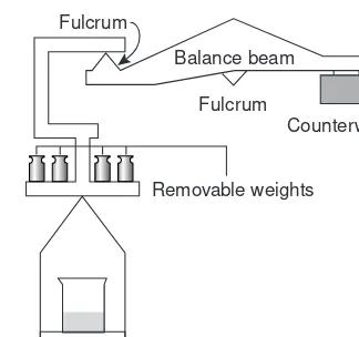
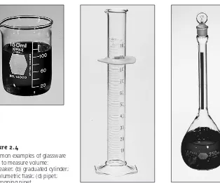
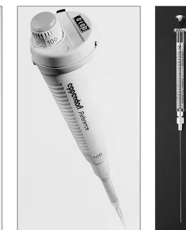
2D Basic Equipment and Instrumentation 25 2D.1 Instrumentation for Measuring Mass 25 2D.2 Equipment for Measuring Volume 26 2D.3 Equipment for Drying Samples 29 2E Preparing Solutions 30
2E.1 Preparing Stock Solutions 30 2E.2 Preparing Solutions by Dilution 31 2F The Laboratory Notebook 32
2G Key Terms 32 2H Summary 33 2I Problems 33
2J Suggested Readings 34 2K References 34
Chapter
3
The Language of Analytical Chemistry 35
3A Analysis, Determination, and Measurement 36 3B Techniques, Methods, Procedures, and
Protocols 36
3C Classifying Analytical Techniques 37 3D Selecting an Analytical Method 38
3D.1 Accuracy 38 3D.2 Precision 39 3D.3 Sensitivity 39 3D.4 Selectivity 40
3D.5 Robustness and Ruggedness 42 3D.6 Scale of Operation 42
4E.4 Errors in Significance Testing 84
4F Statistical Methods for Normal Distributions 85 4F.1 Comparing X–to µ 85
4F.2 Comparing s2to σ2 87
4F.3 Comparing Two Sample Variances 88 4F.4 Comparing Two Sample Means 88 4F.5 Outliers 93
4G Detection Limits 95 4H Key Terms 96 4I Summary 96
4J Suggested Experiments 97 4K Problems 98
4L Suggested Readings 102 4M References 102
Chapter
5
Calibrations, Standardizations,
and Blank Corrections
104
5A Calibrating Signals 105 5B Standardizing Methods 106
5B.1 Reagents Used as Standards 106 5B.2 Single-Point versus Multiple-Point
Standardizations 108 5B.3 External Standards 109 5B.4 Standard Additions 110 5B.5 Internal Standards 115
5C Linear Regression and Calibration Curves 117 5C.1 Linear Regression of Straight-Line Calibration
Curves 118
5C.2 Unweighted Linear Regression with Errors in y 119
5C.3 Weighted Linear Regression with Errors in y 124
5C.4 Weighted Linear Regression with Errors in Both xand y 127
5C.5 Curvilinear and Multivariate Regression 127
5D Blank Corrections 128 5E Key Terms 130 5F Summary 130
5G Suggested Experiments 130 5H Problems 131
5I Suggested Readings 133 5J References 134
3E Developing the Procedure 45
3E.1 Compensating for Interferences 45 3E.2 Calibration and Standardization 47 3E.3 Sampling 47
3E.4 Validation 47 3F Protocols 48
3G The Importance of Analytical Methodology 48 3H Key Terms 50
3I Summary 50 3J Problems 51
3K Suggested Readings 52 3L References 52
Chapter
4
Evaluating Analytical Data 53
4A Characterizing Measurements and Results 54 4A.1 Measures of Central Tendency 54 4A.2 Measures of Spread 55
4B Characterizing Experimental Errors 57 4B.1 Accuracy 57
4B.2 Precision 62
4B.3 Error and Uncertainty 64 4C Propagation of Uncertainty 64
4C.1 A Few Symbols 65
4C.2 Uncertainty When Adding or Subtracting 65 4C.3 Uncertainty When Multiplying or
Dividing 66
4C.4 Uncertainty for Mixed Operations 66 4C.5 Uncertainty for Other Mathematical
Functions 67
4C.6 Is Calculating Uncertainty Actually Useful? 68 4D The Distribution of Measurements and
Results 70
4D.1 Populations and Samples 71
4D.2 Probability Distributions for Populations 71 4D.3 Confidence Intervals for Populations 75 4D.4 Probability Distributions for Samples 77 4D.5 Confidence Intervals for Samples 80 4D.6 A Cautionary Statement 81
4E Statistical Analysis of Data 82 4E.1 Significance Testing 82
4E.2 Constructing a Significance Test 83 4E.3 One-Tailed and Two-Tailed Significance
Chapter
7
Obtaining and Preparing Samples
for Analysis
179
7A The Importance of Sampling 180 7B Designing a Sampling Plan 182
7B.1 Where to Sample the Target Population 182
7B.2 What Type of Sample to Collect 185 7B.3 How Much Sample to Collect 187 7B.4 How Many Samples to Collect 191 7B.5 Minimizing the Overall Variance 192 7C Implementing the Sampling Plan 193
7C.1 Solutions 193 7C.2 Gases 195 7C.3 Solids 196
7D Separating the Analyte from Interferents 201
7E General Theory of Separation Efficiency 202
7F Classifying Separation Techniques 205 7F.1 Separations Based on Size 205
7F.2 Separations Based on Mass or Density 206 7F.3 Separations Based on Complexation
Reactions (Masking) 207 7F.4 Separations Based on a Change
of State 209
7F.5 Separations Based on a Partitioning Between Phases 211
7G Liquid–Liquid Extractions 215
7G.1 Partition Coefficients and Distribution Ratios 216
7G.2 Liquid–Liquid Extraction with No Secondary Reactions 216
7G.3 Liquid–Liquid Extractions Involving Acid–Base Equilibria 219
7G.4 Liquid–Liquid Extractions Involving Metal Chelators 221
7H Separation versus Preconcentration 223 7I Key Terms 224
7J Summary 224
7K Suggested Experiments 225 7L Problems 226
7M Suggested Readings 230 7N References 231
Chapter
6
Equilibrium Chemistry 135
6A Reversible Reactions and Chemical Equilibria 136
6B Thermodynamics and Equilibrium Chemistry 136
6C Manipulating Equilibrium Constants 138 6D Equilibrium Constants for Chemical
Reactions 139
6D.1 Precipitation Reactions 139 6D.2 Acid–Base Reactions 140 6D.3 Complexation Reactions 144 6D.4 Oxidation–Reduction Reactions 145 6E Le Châtelier’s Principle 148
6F Ladder Diagrams 150
6F.1 Ladder Diagrams for Acid–Base Equilibria 150 6F.2 Ladder Diagrams for Complexation
Equilibria 153
6F.3 Ladder Diagrams for Oxidation–Reduction Equilibria 155
6G Solving Equilibrium Problems 156
6G.1 A Simple Problem: Solubility of Pb(IO3)2in Water 156
6G.2 A More Complex Problem: The Common Ion Effect 157
6G.3 Systematic Approach to Solving Equilibrium Problems 159
6G.4 pH of a Monoprotic Weak Acid 160 6G.5 pH of a Polyprotic Acid or Base 163 6G.6 Effect of Complexation on Solubility 165 6H Buffer Solutions 167
6H.1 Systematic Solution to Buffer Problems 168
6H.2 Representing Buffer Solutions with Ladder Diagrams 170
6I Activity Effects 171
6J Two Final Thoughts About Equilibrium Chemistry 175
6K Key Terms 175 6L Summary 175
6M Suggested Experiments 176 6N Problems 176
Chapter
8
Gravimetric Methods of Analysis
232
8A Overview of Gravimetry 233 8A.1 Using Mass as a Signal 233 8A.2 Types of Gravimetric Methods 234 8A.3 Conservation of Mass 234
8A.4 Why Gravimetry Is Important 235 8B Precipitation Gravimetry 235
8B.1 Theory and Practice 235 8B.2 Quantitative Applications 247 8B.3 Qualitative Applications 254
8B.4 Evaluating Precipitation Gravimetry 254 8C Volatilization Gravimetry 255
8C.1 Theory and Practice 255 8C.2 Quantitative Applications 259
8C.3 Evaluating Volatilization Gravimetry 262 8D Particulate Gravimetry 262
8D.1 Theory and Practice 263 8D.2 Quantitative Applications 264
8D.3 Evaluating Precipitation Gravimetry 265 8E Key Terms 265
8F Summary 266
8G Suggested Experiments 266 8H Problems 267
8I Suggested Readings 271 8J References 272
Chapter
9
Titrimetric Methods of Analysis 273
9A Overview of Titrimetry 274
9A.1 Equivalence Points and End Points 274 9A.2 Volume as a Signal 274
9A.3 Titration Curves 275 9A.4 The Buret 277
9B Titrations Based on Acid–Base Reactions 278 9B.1 Acid–Base Titration Curves 279
9B.2 Selecting and Evaluating the End Point 287
9B.3 Titrations in Nonaqueous Solvents 295 9B.4 Representative Method 296
9B.5 Quantitative Applications 298 9B.6 Qualitative Applications 308
9B.7 Characterization Applications 309 9B.8 Evaluation of Acid–Base Titrimetry 311 9C Titrations Based on Complexation Reactions 314
9C.1 Chemistry and Properties of EDTA 315 9C.2 Complexometric EDTA Titration Curves 317 9C.3 Selecting and Evaluating the End Point 322 9C.4 Representative Method 324
9C.5 Quantitative Applications 327
9C.6 Evaluation of Complexation Titrimetry 331 9D Titrations Based on Redox Reactions 331
9D.1 Redox Titration Curves 332
9D.2 Selecting and Evaluating the End Point 337 9D.3 Representative Method 340
9D.4 Quantitative Applications 341 9D.5 Evaluation of Redox Titrimetry 350 9E Precipitation Titrations 350
9E.1 Titration Curves 350
9E.2 Selecting and Evaluating the End Point 354 9E.3 Quantitative Applications 354
9E.4 Evaluation of Precipitation Titrimetry 357 9F Key Terms 357
9G Summary 357
9H Suggested Experiments 358 9I Problems 360
9J Suggested Readings 366 9K References 367
Chapter
10
Spectroscopic Methods
of Analysis
368
10A Overview of Spectroscopy 369
10A.1 What Is Electromagnetic Radiation 369 10A.2 Measuring Photons as a Signal 372 10B Basic Components of Spectroscopic
Instrumentation 374 10B.1 Sources of Energy 375 10B.2 Wavelength Selection 376 10B.3 Detectors 379
10B.4 Signal Processors 380
10C Spectroscopy Based on Absorption 380
10C.1 Absorbance of Electromagnetic Radiation 380 10C.2 Transmittance and Absorbance 384 10C.3 Absorbance and Concentration: Beer’s
11B Potentiometric Methods of Analysis 465 11B.1 Potentiometric Measurements 466 11B.2 Reference Electrodes 471
11B.3 Metallic Indicator Electrodes 473 11B.4 Membrane Electrodes 475 11B.5 Quantitative Applications 485 11B.6 Evaluation 494
11C Coulometric Methods of Analysis 496 11C.1 Controlled-Potential Coulometry 497 11C.2 Controlled-Current Coulometry 499 11C.3 Quantitative Applications 501 11C.4 Characterization Applications 506 11C.5 Evaluation 507
11D Voltammetric Methods of Analysis 508 11D.1 Voltammetric Measurements 509 11D.2 Current in Voltammetry 510 11D.3 Shape of Voltammograms 513 11D.4 Quantitative and Qualitative Aspects
of Voltammetry 514 11D.5 Voltammetric Techniques 515 11D.6 Quantitative Applications 520 11D.7 Characterization Applications 527 11D.8 Evaluation 531
11E Key Terms 532 11F Summary 532
11G Suggested Experiments 533 11H Problems 535
11I Suggested Readings 540 11J References 541
Chapter
12
Chromatographic and Electrophoretic
Methods 543
12A Overview of Analytical Separations 544 12A.1 The Problem with Simple
Separations 544
12A.2 A Better Way to Separate Mixtures 544 12A.3 Classifying Analytical Separations 546 12B General Theory of Column
Chromatography 547
12B.1 Chromatographic Resolution 549 12B.2 Capacity Factor 550
12B.3 Column Selectivity 552 12B.4 Column Efficiency 552 10C.4 Beer’s Law and Multicomponent
Samples 386
10C.5 Limitations to Beer’s Law 386 10D Ultraviolet-Visible and Infrared
Spectrophotometry 388 10D.1 Instrumentation 388
10D.2 Quantitative Applications 394 10D.3 Qualitative Applications 402 10D.4 Characterization Applications 403 10D.5 Evaluation 409
10E Atomic Absorption Spectroscopy 412 10E.1 Instrumentation 412
10E.2 Quantitative Applications 415 10E.3 Evaluation 422
10F Spectroscopy Based on Emission 423 10G Molecular Photoluminescence
Spectroscopy 423
10G.1 Molecular Fluorescence and Phosphorescence Spectra 424 10G.2 Instrumentation 427
10G.3 Quantitative Applications Using Molecular Luminescence 429
10G.4 Evaluation 432
10H Atomic Emission Spectroscopy 434 10H.1 Atomic Emission Spectra 434 10H.2 Equipment 435
10H.3 Quantitative Applications 437 10H.4 Evaluation 440
10I Spectroscopy Based on Scattering 441 10I.1 Origin of Scattering 441
10I.2 Turbidimetry and Nephelometry 441 10J Key Terms 446
10K Summary 446
10L Suggested Experiments 447 10M Problems 450
10N Suggested Readings 458 10O References 459
Chapter
11
Electrochemical Methods of Analysis 461
11A Classification of Electrochemical Methods 462 11A.1 Interfacial Electrochemical Methods 462 11A.2 Controlling and Measuring Current and
12B.5 Peak Capacity 554 12B.6 Nonideal Behavior 555
12C Optimizing Chromatographic Separations 556 12C.1 Using the Capacity Factor to Optimize
Resolution 556
12C.2 Using Column Selectivity to Optimize Resolution 558
12C.3 Using Column Efficiency to Optimize Resolution 559
12D Gas Chromatography 563 12D.1 Mobile Phase 563
12D.2 Chromatographic Columns 564 12D.3 Stationary Phases 565
12D.4 Sample Introduction 567 12D.5 Temperature Control 568
12D.6 Detectors for Gas Chromatography 569 12D.7 Quantitative Applications 571
12D.8 Qualitative Applications 575 12D.9 Representative Method 576 12D.10 Evaluation 577
12E High-Performance Liquid Chromatography 578 12E.1 HPLC Columns 578 12E.2 Stationary Phases 579 12E.3 Mobile Phases 580 12E.4 HPLC Plumbing 583 12E.5 Sample Introduction 584 12E.6 Detectors for HPLC 584 12E.7 Quantitative Applications 586 12E.8 Representative Method 588 12E.9 Evaluation 589
12F Liquid–Solid Adsorption Chromatography 590 12G Ion-Exchange Chromatography 590
12H Size-Exclusion Chromatography 593 12I Supercritical Fluid Chromatography 596 12J Electrophoresis 597
12J.1 Theory of Capillary Electrophoresis 598 12J.2 Instrumentation 601
12J.3 Capillary Electrophoresis Methods 604 12J.4 Representative Method 607
12J.5 Evaluation 609 12K Key Terms 609 12L Summary 610
12M Suggested Experiments 610 12N Problems 615
12O Suggested Readings 620 12P References 620
Chapter
13
Kinetic Methods of Analysis
622
13A Methods Based on Chemical Kinetics 623 13A.1 Theory and Practice 624
13A.2 Instrumentation 634
13A.3 Quantitative Applications 636 13A.4 Characterization Applications 638 13A.5 Evaluation of Chemical Kinetic
Methods 639
13B Radiochemical Methods of Analysis 642 13B.1 Theory and Practice 643
13B.2 Instrumentation 643
13B.3 Quantitative Applications 644 13B.4 Characterization Applications 647 13B.5 Evaluation 648
13C Flow Injection Analysis 649 13C.1 Theory and Practice 649 13C.2 Instrumentation 651
13C.3 Quantitative Applications 655 13C.4 Evaluation 658
13D Key Terms 658 13E Summary 659
13F Suggested Experiments 659 13G Problems 661
13H Suggested Readings 664 13I References 665
Chapter
14
Developing a Standard Method 666
14A Optimizing the Experimental Procedure 667 14A.1 Response Surfaces 667
14A.2 Searching Algorithms for Response Surfaces 668
14A.3 Mathematical Models of Response Surfaces 674
14B Verifying the Method 683
14B.1 Single-Operator Characteristics 683 14B.2 Blind Analysis of Standard Samples 683 14B.3 Ruggedness Testing 684
15D Key Terms 721 15E Summary 722
15F Suggested Experiments 722 15G Problems 722
15H Suggested Readings 724 15I References 724
Appendixes
Appendix 1A Single-Sided Normal Distribution 725
Appendix 1B t-Table 726
Appendix 1C F-Table 727
Appendix 1D Critical Values for Q-Test 728
Appendix 1E Random Number Table 728
Appendix 2 Recommended Reagents for Preparing Primary Standards 729
Appendix 3A Solubility Products 731
Appendix 3B Acid Dissociation Constants 732
Appendix 3C Metal–Ligand Formation Constants 739
Appendix 3D Standard Reduction Potentials 743
Appendix 3E Selected Polarographic Half-Wave Potentials 747
Appendix 4 Balancing Redox Reactions 748
Appendix 5 Review of Chemical Kinetics 750
Appendix 6 Countercurrent Separations 755
Appendix 7 Answers to Selected Problems 762
Glossary 769 Index 781 14C Validating the Method as a Standard
Method 687
14C.1 Two-Sample Collaborative Testing 688 14C.2 Collaborative Testing and Analysis of
Variance 693
14C.3 What Is a Reasonable Result for a Collaborative Study? 698 14D Key Terms 699
14E Summary 699
14F Suggested Experiments 699 14G Problems 700
14H Suggested Readings 704 14I References 704
Chapter
15
Quality Assurance
705
15A Quality Control 706 15B Quality Assessment 708
15B.1 Internal Methods of Quality Assessment 708
15B.2 External Methods of Quality Assessment 711
15C Evaluating Quality Assurance Data 712 15C.1 Prescriptive Approach 712
A Guide to Using This Text
. . . in Chapter
Representative Methods
Annotated methods of typical analytical procedures link theory with practice. The format encourages students to think about the design of the procedure and why it works.246 Modern Analytical Chemistry
Representative Methods
An additional problem is encountered when the isolated solid is non-stoichiometric. For example, precipitating Mn2+as Mn(OH)
2, followed by heating
to produce the oxide, frequently produces a solid with a stoichiometry of MnOx, where xvaries between 1 and 2. In this case the nonstoichiometric product results from the formation of a mixture of several oxides that differ in the oxidation state of manganese. Other nonstoichiometric compounds form as a result of lattice de-fects in the crystal structure.6
Representative Method The best way to appreciate the importance of the theoreti-cal and practitheoreti-cal details discussed in the previous section is to carefully examine the procedure for a typical precipitation gravimetric method. Although each method has its own unique considerations, the determination of Mg2+in water and
waste-water by precipitating MgNH4PO4⋅6H2O and isolating Mg2P2O7provides an
in-structive example of a typical procedure.
Method 8.1 Determination of Mg2+in Water and Wastewater7
Description of Method. Magnesium is precipitated as MgNH4PO4⋅6H2O using (NH4)2HPO4as the precipitant. The precipitate’s solubility in neutral solutions (0.0065 g/100 mL in pure water at 10 °C) is relatively high, but it is much less soluble in the presence of dilute ammonia (0.0003 g/100 mL in 0.6 M NH3). The precipitant is not very selective, so a preliminary separation of Mg2+from potential interferents is necessary. Calcium, which is the most significant interferent, is usually removed by its prior precipitation as the oxalate. The presence of excess ammonium salts from the precipitant or the addition of too much ammonia can lead to the formation of Mg(NH4)4(PO4)2, which is subsequently isolated as Mg(PO3)2after drying. The precipitate is isolated by filtration using a rinse solution of dilute ammonia. After filtering, the precipitate is converted to Mg2P2O7 and weighed.
Procedure. Transfer a sample containing no more than 60 mg of Mg2+into a 600-mL beaker. Add 2–3 drops of methyl red indicator, and, if necessary, adjust the volume to 150 mL. Acidify the solution with 6 M HCl, and add 10 mL of 30% w/v (NH4)2HPO4. After cooling, add concentrated NH3dropwise, and while constantly stirring, until the methyl red indicator turns yellow (pH > 6.3). After stirring for 5 min, add 5 mL of concentrated NH3, and continue stirring for an additional 10 min. Allow the resulting solution and precipitate to stand overnight. Isolate the precipitate by filtration, rinsing with 5% v/v NH3. Dissolve the precipitate in 50 mL of 10% v/v HCl, and precipitate a second time following the same procedure. After filtering, carefully remove the filter paper by charring. Heat the precipitate at 500 °C until the residue is white, and then bring the precipitate to constant weight at 1100 °C.
Questions
1. Why does the procedure call for a sample containing no more than 60 mg of
q y
There is a serious limitation, however, to an external standardization. The relationship between Sstandand CSin equation 5.3 is determined when the
ana-lyte is present in the external standard’s matrix. In using an external standardiza-tion, we assume that any difference between the matrix of the standards and the sample’s matrix has no effect on the value of k.A proportional determinate error is introduced when differences between the two matrices cannot be ignored. This is shown in Figure 5.4, where the relationship between the signal and the amount of analyte is shown for both the sample’s matrix and the standard’s matrix. In this example, using a normal calibration curve results in a negative determinate error. When matrix problems are expected, an effort is made to match the matrix of the standards to that of the sample. This is known as matrix matching.When the sample’s matrix is unknown, the matrix effect must be shown to be negligi-ble, or an alternative method of standardization must be used. Both approaches are discussed in the following sections.
5B.4Standard Additions
The complication of matching the matrix of the standards to that of the sample can be avoided by conducting the standardization in the sample. This is known as the method of standard additions.The simplest version of a standard addi-tion is shown in Figure 5.5. A volume, Vo, of sample is diluted to a final volume, Vf, and the signal, Ssampis measured. A second identical aliquotof sample is
matrix matching
Adjusting the matrix of an external standard so that it is the same as the matrix of the samples to be analyzed.
method of standard additions
A standardization in which aliquots of a standard solution are added to the sample.
Examples of Typical Problems
Each example problem includes a detailed solution that helps students in applying the chapter’s material to practical problems.Margin Notes
Margin notes direct students to colorplates located toward the middle of the bookBold-faced Key Terms with Margin Definitions
Key words appear in boldface when they are introduced within the text. The term and its definition appear in the margin for quick review by the student. All key words are also defined in the glossary.110 Modern Analytical Chemistry
either case, the calibration curve provides a means for relating Ssampto the
ana-lyte’s concentration. EXAMPLE 5.3
A second spectrophotometric method for the quantitative determination of Pb2+levels in blood gives a linear normal calibration curve for which
Sstand= (0.296 ppb–1)×CS+ 0.003
What is the Pb2+level (in ppb) in a sample of blood if S sampis 0.397? SOLUTION
To determine the concentration of Pb2+in the sample of blood, we replace Sstandin the calibration equation with Ssampand solve for CA
It is worth noting that the calibration equation in this problem includes an extra term that is not in equation 5.3. Ideally, we expect the calibration curve to give a signal of zero when CSis zero. This is the purpose of using a reagent
blank to correct the measured signal. The extra term of +0.003 in our calibration equation results from uncertainty in measuring the signal for the reagent blank and the standards.
An external standardization allows a related series of samples to be analyzed using a single calibration curve. This is an important advantage in laboratories where many samples are to be analyzed or when the need for a rapid throughput of l i iti l t i i l f th t l t d Color plate 1 shows an example of a set of
external standards and their corresponding normal calibration curve.
List of Key Terms
The key terms introduced within the chapter are listed at the end of each chapter. Page references direct the student to the definitions in the text.
Summary
The summary provides the student with a brief review of the important concepts within the chapter.
Suggested Experiments
An annotated list of representative experiments is provided from the Journal of Chemical Education.
y y
5E KEY TERMS aliquot (p. 111) external standard (p. 109) internal standard (p. 116) linear regression (p. 118) matrix matching (p. 110) method of standard additions (p. 110)
multiple-point standardization (p. 109) normal calibration curve (p. 109) primary reagent (p. 106) reagent grade (p. 107) residual error (p. 118)
secondary reagent (p. 107) single-point standardization (p. 108) standard deviation about the
regression (p. 121) total Youden blank (p. 129)
In a quantitative analysis, we measure a signal and calculate the amount of analyte using one of the following equations.
Smeas=knA+Sreag Smeas=kCA+Sreag
To obtain accurate results we must eliminate determinate errors affecting the measured signal, Smeas, the method’s sensitivity, k, and any signal due to the reagents, Sreag.
To ensure that Smeasis determined accurately, we calibrate the equipment or instrument used to obtain the signal. Balances are calibrated using standard weights. When necessary, we can also correct for the buoyancy of air. Volumetric glassware can be calibrated by measuring the mass of water contained or de-livered and using the density of water to calculate the true vol-ume. Most instruments have calibration standards suggested by the manufacturer.
An analytical method is standardized by determining its sensi-tivity. There are several approaches to standardization, including the use of external standards, the method of standard addition,
and the use of an internal standard. The most desirable standard-ization strategy is an external standardstandard-ization. The method of standard additions, in which known amounts of analyte are added to the sample, is used when the sample’s matrix complicates the analysis. An internal standard, which is a species (not analyte) added to all samples and standards, is used when the procedure does not allow for the reproducible handling of samples and standards.
Standardizations using a single standard are common, but also are subject to greater uncertainty. Whenever possible, a multiple-point standardization is preferred. The results of a multiple-multiple-point standardization are graphed as a calibration curve. A linear regres-sion analysis can provide an equation for the standardization.
A reagent blank corrects the measured signal for signals due to reagents other than the sample that are used in an analysis. The most common reagent blank is prepared by omitting the sample. When a simple reagent blank does not compensate for all constant sources of determinate error, other types of blanks, such as the total Youden blank, can be used.
5F SUMMARY
Calibration—Volumetric glassware (burets, pipets, and volumetric flasks) can be calibrated in the manner described in Example 5.1. Most instruments have a calibration sample that can be prepared to verify the instrument’s accuracy and precision. For example, as described in this chapter, a solution of 60.06 ppm K2Cr2O7in 0.0050 M H2SO4should give an absorbance of 0.640± 0.010 at a wavelength of 350.0 nm when using 0.0050 M H2SO4as a reagent blank. These exercises also provide practice with using volumetric glassware, weighing samples, and preparing solutions.
Standardization—External standards, standard additions, and internal standards are a common feature of many quantitative analyses. Suggested experiments using these standardization methods are found in later chapters. A good project experiment for introducing external standardization, standard additions, and the importance of the sample’s matrix is to explore the effect of pH on the quantitative analysis of an acid–base indicator. Using bromothymol blue as an example, external standards can be prepared in a pH 9 buffer and used to analyze samples buffered to different pHs in the range of 6–10. Results can be compared with those obtained using a standard addition.
5G SuggestedEXPERIMENTS
The following exercises and experiments help connect the material in this chapter to the analytical laboratory.
Experiments
1.When working with a solid sample, it often is necessary to bring the analyte into solution by dissolving the sample in a suitable solvent. Any solid impurities that remain are removed by filtration before continuing with the analysis. In a typical total analysis method, the procedure might read
After dissolving the sample in a beaker, remove any solid impurities by passing the solution containing the analyte through filter paper, collecting the solution in a clean Erlenmeyer flask. Rinse the beaker with several small portions of solvent, passing these rinsings through the filter paper, and collecting them in the same Erlenmeyer flask. Finally, rinse the filter paper with several portions of solvent, collecting the rinsings in the same Erlenmeyer flask.
For a typical concentration method, however, the procedure might state
4.A sample was analyzed to determine the concentration of an analyte. Under the conditions of the analysis, the sensitivity is 17.2 ppm–1. What is the analyte’s concentration if Smeasis 35.2 and Sreagis 0.6?
5.A method for the analysis of Ca2+in water suffers from an interference in the presence of Zn2+. When the concentration of Ca2+is 50 times greater than that of Zn2+, an analysis for Ca2+gives a relative error of –2.0%. What is the value of the selectivity coefficient for this method?
6.The quantitative analysis for reduced glutathione in blood is complicated by the presence of many potential interferents. In one study, when analyzing a solution of 10-ppb glutathione and 1.5-ppb ascorbic acid, the signal was 5.43 times greater than that obtained for the analysis of 10-ppb glutathione.12What is the selectivity coefficient for this analysis? The same study found that when analyzing a solution of 350-ppb methionine and 10-ppb glutathione the signal was 0 906 times less than that obtained for the analysis 3J PROBLEMS
y y
The role of analytical chemistry within the broader discipline of chemistry has been discussed by many prominent analytical chemists. Several notable examples follow. Baiulescu, G. E.; Patroescu, C.; Chalmers, R. A. Education and
Teaching in Analytical Chemistry.Ellis Horwood: Chichester, 1982.
Hieftje, G. M. “The Two Sides of Analytical Chemistry,” Anal. Chem.1985,57,256A–267A.
Kissinger, P. T. “Analytical Chemistry—What is It? Who Needs It? Why Teach It?” Trends Anal. Chem.1992,11,54–57.
Laitinen, H. A. “Analytical Chemistry in a Changing World,” Anal. Chem.1980,52,605A–609A.
Laitinen, H. A. “History of Analytical Chemistry in the U.S.A.,” Talanta1989,36,1–9.
Laitinen, H. A.; Ewing, G. (eds). A History of Analytical Chemistry.The Division of Analytical Chemistry of the American Chemical Society: Washington, D.C., 1972.
McLafferty, F. W. “Analytical Chemistry: Historic and Modern,” Acc. Chem. Res.1990,23,63–64.
1G SUGGESTED READINGS
1. Ravey, M. Spectroscopy1990,5(7),11. 2. de Haseth, J. Spectroscopy1990,5(7),11.
3. Fresenius, C. R. A System of Instruction in Quantitative Chemical Analysis.John Wiley and Sons: New York, 1881. 4. Hillebrand, W. F.; Lundell, G. E. F. Applied Inorganic Analysis,John
Wiley and Sons: New York, 1953.
5. Van Loon, J. C. Analytical Atomic Absorption Spectroscopy.Academic Press: New York, 1980.
6. Murray, R. W. Anal. Chem.1991,63,271A.
7. For several different viewpoints see (a) Beilby, A. L. J. Chem. Educ. 1970,47,237–238; (b) Lucchesi, C. A. Am. Lab.1980,October,
113–119; (c) Atkinson, G. F. J. Chem. Educ.1982,59,201–202; (d) Pardue, H. L.; Woo, J. J. Chem. Educ.1984,61,409–412; (e) Guarnieri, M. J. Chem. Educ.1988,65,201–203; (f) de Haseth, J. Spectroscopy1990,5,20–21; (g) Strobel, H. A. Am. Lab.1990, October,17–24.
8. Hieftje, G. M. Am. Lab.1993,October,53–61. 9. See, for example, the following laboratory texts: (a) Sorum, C. H.;
Lagowski, J. J. Introduction to Semimicro Qualitative Analysis,5th ed. Prentice-Hall: Englewood Cliffs, NJ, 1977.; (b) Shriner, R. L.; Fuson, R. C.; Curtin, D. Y. The Systematic Identification of Organic Compounds,5th ed. John Wiley and Sons: New York, 1964. 1H REFERENCES
Problems
A variety of problems, many based on data from the analytical literature, provide the student with practical examples of current research.
Suggested Readings
Suggested readings give the student access to more comprehensive discussion of the topics introduced within the chapter.References
The references cited in the chapter are provided so the student can access them for further information.
A
s currently taught, the introductory course in analytical chemistry emphasizes quantitative (and sometimes qualitative) methods of analysis coupled with a heavy dose of equilibrium chemistry. Analytical chemistry, however, is more than equilib-rium chemistry and a collection of analytical methods; it is an approach to solving chemical problems. Although discussing different methods is important, that dis-cussion should not come at the expense of other equally important topics. The intro-ductory analytical course is the ideal place in the chemistry curriculum to explore topics such as experimental design, sampling, calibration strategies, standardization, optimization, statistics, and the validation of experimental results. These topics are important in developing good experimental protocols, and in interpreting experi-mental results. If chemistry is truly an experiexperi-mental science, then it is essential that all chemistry students understand how these topics relate to the experiments they conduct in other chemistry courses.Currently available textbooks do a good job of covering the diverse range of wet and instrumental analysis techniques available to chemists. Although there is some disagreement about the proper balance between wet analytical techniques, such as gravimetry and titrimetry, and instrumental analysis techniques, such as spec-trophotometry, all currently available textbooks cover a reasonable variety of tech-niques. These textbooks, however, neglect, or give only brief consideration to, obtaining representative samples, handling interferents, optimizing methods, ana-lyzing data, validating data, and ensuring that data are collected under a state of sta-tistical control.
In preparing this textbook, I have tried to find a more appropriate balance between theory and practice, between “classical” and “modern” methods of analysis, between analyzing samples and collecting and preparing samples for analysis, and between analytical methods and data analysis. Clearly, the amount of material in this textbook exceeds what can be covered in a single semester; it’s my hope, however, that the diversity of topics will meet the needs of different instructors, while, per-haps, suggesting some new topics to cover.
The anticipated audience for this textbook includes students majoring in chem-istry, and students majoring in other science disciplines (biology, biochemchem-istry, environmental science, engineering, and geology, to name a few), interested in obtaining a stronger background in chemical analysis. It is particularly appropriate for chemistry majors who are not planning to attend graduate school, and who often do not enroll in those advanced courses in analytical chemistry that require physical chemistry as a pre-requisite. Prior coursework of a year of general chemistry is assumed. Competence in algebra is essential; calculus is used on occasion, however, its presence is not essential to the material’s treatment.
xii
Key Features of This Textbook
Key features set this textbook apart from others currently available.
• A stronger emphasis on the evaluation of data.Methods for characterizing chemical measurements, results, and errors (including the propagation of errors) are included. Both the binomial distribution and normal distribution are presented, and the idea of a confidence interval is developed. Statistical methods for evaluating data include the t-test (both for paired and unpaired data), the F-test, and the treatment of outliers. Detection limits also are discussed from a statistical perspective. Other statistical methods, such as ANOVA and ruggedness testing, are presented in later chapters.
• Standardizations and calibrations are treated in a single chapter.Selecting the most appropriate calibration method is important and, for this reason, the methods of external standards, standard additions, and internal standards are gathered together in a single chapter. A discussion of curve-fitting, including the statistical basis for linear regression (with and without weighting) also is included in this chapter.
• More attention to selecting and obtaining a representative sample.The design of a statistically based sampling plan and its implementation are discussed earlier, and in more detail than in other textbooks. Topics that are covered include how to obtain a representative sample, how much sample to collect, how many samples to collect, how to minimize the overall variance for an analytical method, tools for collecting samples, and sample preservation.
• The importance of minimizing interferents is emphasized.Commonly used methods for separating interferents from analytes, such as distillation, masking, and solvent extraction, are gathered together in a single chapter.
• Balanced coverage of analytical techniques.The six areas of analytical techniques—gravimetry, titrimetry, spectroscopy, electrochemistry,
chromatography, and kinetics—receive roughly equivalent coverage, meeting the needs of instructors wishing to emphasize wet methods and those
emphasizing instrumental methods. Related methods are gathered together in a single chapter encouraging students to see the similarities between methods, rather than focusing on their differences.
• An emphasis on practical applications.Throughout the text applications from organic chemistry, inorganic chemistry, environmental chemistry, clinical chemistry, and biochemistry are used in worked examples, representative methods, and end-of-chapter problems.
• Representative methods link theory with practice.An important feature of this text is the presentation of representative methods. These boxed features present typical analytical procedures in a format that encourages students to think about why the procedure is designed as it is.
• Problems adapted from the literature.Many of the in-chapter examples and end-of-chapter problems are based on data from the analytical literature, providing students with practical examples of current research in analytical chemistry. • An emphasis on critical thinking.Critical thinking is encouraged through
problems in which students are asked to explain why certain steps in an analytical procedure are included, or to determine the effect of an experimental error on the results of an analysis.
• Suggested experiments from the Journal of Chemical Education.Rather than including a short collection of experiments emphasizing the analysis of standard unknowns, an annotated list of representative experiments from the
Journal of Chemical Educationis included at the conclusion of most chapters. These experiments may serve as stand alone experiments, or as starting points for individual or group projects.
The Role of Equilibrium Chemistry in Analytical Chemistry
Equilibrium chemistry often receives a significant emphasis in the introductory ana-lytical chemistry course. While an important topic, its overemphasis can cause stu-dents to confuse analytical chemistry with equilibrium chemistry. Although atten-tion to solving equilibrium problems is important, it is equally important for stu-dents to recognize when such calculations are impractical, or when a simpler, more qualitative approach is all that is needed. For example, in discussing the gravimetric analysis of Ag+as AgCl, there is little point in calculating the equilibrium solubility
of AgCl since the concentration of Cl–at equilibrium is rarely known. It is
impor-tant, however, to qualitatively understand that a large excess of Cl–increases the
sol-ubility of AgCl due to the formation of soluble silver-chloro complexes. Balancing the presentation of a rigorous approach to solving equilibrium problems, this text also introduces the use of ladder diagrams as a means for providing a qualitative pic-ture of a system at equilibrium. Students are encouraged to use the approach best suited to the problem at hand.
Computer Software
Many of the topics covered in analytical chemistry benefit from the availability of appropriate computer software. In preparing this text, however, I made a conscious decision to avoid a presentation tied to a single computer platform or software pack-age. Students and faculty are increasingly experienced in the use of computers, spreadsheets, and data analysis software; their use is, I think, best left to the person-al choice of each student and instructor.
Organization
The textbook’s organization can be divided into four parts. Chapters 1–3 serve as an introduction, providing an overview of analytical chemistry (Chapter 1); a review of the basic tools of analytical chemistry, including significant figures, units, and stoi-chiometry (Chapter 2); and an introduction to the terminology used by analytical chemists (Chapter 3). Familiarity with the material in these chapters is assumed throughout the remainder of the text.
of these chapters, as needed, to support individual course goals. The statistical analy-sis of data is covered in Chapter 4 at a level that is more complete than that found in other introductory analytical textbooks. Methods for calibrating equipment, stan-dardizing methods, and linear regression are gathered together in Chapter 5. Chapter 6 provides an introduction to equilibrium chemistry, stressing both the rigorous solution to equilibrium problems, and the use of semi-quantitative approaches, such as ladder diagrams. The importance of collecting the right sample, and methods for separating analytes and interferents are covered in Chapter 7.
Chapters 8–13 cover the major areas of analysis, including gravimetry (Chapter 8), titrimetry (Chapter 9), spectroscopy (Chapter 10), electrochemistry (Chapter 11), chromatography and electrophoresis (Chapter 12), and kinetic meth-ods (Chapter 13). Related techniques, such as acid–base titrimetry and redox titrimetry, or potentiometry and voltammetry, are gathered together in single chap-ters. Combining related techniques together encourages students to see the similar-ities between methods, rather than focusing on their differences. The first technique presented in each chapter is generally that which is most commonly covered in the introductory course.
Finally, the textbook concludes with two chapters discussing the design and maintenance of analytical methods, two topics of importance to analytical chemists. Chapter 14 considers the development of an analytical method, including its opti-mization, verification, and validation. Quality control and quality assessment are discussed in Chapter 15.
Acknowledgments
Before beginning an academic career I was, of course, a student. My interest in chemistry and teaching was nurtured by many fine teachers at Westtown Friends School, Knox College, and the University of North Carolina at Chapel Hill; their col-lective influence continues to bear fruit. In particular, I wish to recognize David MacInnes, Alan Hiebert, Robert Kooser, and Richard Linton.
I have been fortunate to work with many fine colleagues during my nearly 17 years of teaching undergraduate chemistry at Stockton State College and DePauw University. I am particularly grateful for the friendship and guidance provided by Jon Griffiths and Ed Paul during my four years at Stockton State College. At DePauw University, Jim George and Bryan Hanson have willingly shared their ideas about teaching, while patiently listening to mine.
Approximately 300 students have joined me in thinking and learning about ana-lytical chemistry; their questions and comments helped guide the development of this textbook. I realize that working without a formal textbook has been frustrating and awkward; all the more reason why I appreciate their effort and hard work.
The following individuals reviewed portions of this textbook at various stages during its development.
David Ballantine
Northern Illinois University
John E. Bauer
Illinois State University
Ali Bazzi
University of Michigan–Dearborn
Steven D. Brown
University of Delaware
Wendy Clevenger
University of Tennessee–Chattanooga
Cathy Cobb
Augusta State University
Paul Flowers
University of North Carolina–Pembroke
Nancy Gordon
Virginia M. Indivero
Swarthmore College
Michael Janusa
Nicholls State University
J. David Jenkins
Georgia Southern University
Richard S. Mitchell
Arkansas State University
George A. Pearse, Jr.
Le Moyne College
Gary Rayson
New Mexico State University
David Redfield
NW Nazarene University
I am particularly grateful for their detailed written comments and suggestions for improving the manuscript. Much of what is good in the final manuscript is the result of their interest and ideas. George Foy (York College of Pennsylvania), John McBride (Hofstra University), and David Karpovich (Saginaw Valley State University) checked the accuracy of problems in the textbook. Gary Kinsel (University of Texas at Arlington) reviewed the page proofs and provided additional suggestions.
This project began in the summer of 1992 with the support of a course develop-ment grant from DePauw University’s Faculty Developdevelop-ment Fund. Additional finan-cial support from DePauw University’s Presidential Discretionary Fund also is acknowledged. Portions of the first draft were written during a sabbatical leave in the Fall semester of the 1993/94 academic year. A Fisher Fellowship provided release time during the Fall 1995 semester to complete the manuscript’s second draft.
Alltech and Associates (Deerfield, IL) graciously provided permission to use the chromatograms in Chapter 12; the assistance of Jim Anderson, Vice-President, and Julia Poncher, Publications Director, is greatly appreciated. Fred Soster and Marilyn Culler, both of DePauw University, provided assistance with some of the photographs.
The editorial staff at McGraw-Hill has helped guide a novice through the process of developing this text. I am particularly thankful for the encouragement and confidence shown by Jim Smith, Publisher for Chemistry, and Kent Peterson, Sponsoring Editor for Chemistry. Shirley Oberbroeckling, Developmental Editor for Chemistry, and Jayne Klein, Senior Project Manager, patiently answered my ques-tions and successfully guided me through the publishing process.
Finally, I would be remiss if I did not recognize the importance of my family’s support and encouragement, particularly that of my parents. A very special thanks to my daughter, Devon, for gifts too numerous to detail.
How to Contact the Author
Writing this textbook has been an interesting (and exhausting) challenge. Despite my efforts, I am sure there are a few glitches, better examples, more interesting end-of-chapter problems, and better ways to think about some of the topics. I welcome your comments, suggestions, and data for interesting problems, which may be addressed to me at DePauw University, 602 S. College St., Greencastle, IN 46135, or electronically at [email protected].
Vincent Remcho
West Virginia University
Jeanette K. Rice
Georgia Southern University
Martin W. Rowe
Texas A&M University
Alexander Scheeline
University of Illinois
James D. Stuart
University of Connecticut
Thomas J. Wenzel
Bates College
David Zax
C
Ch
ha
ap
ptteerr
1
1
Introduction
C
hemistry is the study of matter, including its composition,
structure, physical properties, and reactivity. There are many
approaches to studying chemistry, but, for convenience, we
traditionally divide it into five fields: organic, inorganic, physical,
biochemical, and analytical. Although this division is historical and
arbitrary, as witnessed by the current interest in interdisciplinary areas
such as bioanalytical and organometallic chemistry, these five fields
remain the simplest division spanning the discipline of chemistry.
*Attributed to C. N. Reilley (1925–1981) on receipt of the 1965 Fisher Award in Analytical Chemistry. Reilley, who was a professor of chemistry at the University of North Carolina at Chapel Hill, was one of the most influential analytical chemists of the last half of the twentieth century.
1A
What Is Analytical Chemistry?
“Analytical chemistry is what analytical chemists do.”*
We begin this section with a deceptively simple question. What is analytical chem-istry? Like all fields of chemistry, analytical chemistry is too broad and active a disci-pline for us to easily or completely define in an introductory textbook. Instead, we will try to say a little about what analytical chemistry is, as well as a little about what analytical chemistry is not.
Analytical chemistry is often described as the area of chemistry responsible for characterizing the composition of matter, both qualitatively (what is present) and quantitatively (how much is present). This description is misleading. After all, al-most all chemists routinely make qualitative or quantitative measurements. The ar-gument has been made that analytical chemistry is not a separate branch of chem-istry, but simply the application of chemical knowledge.1In fact, you probably have performed quantitative and qualitative analyses in other chemistry courses. For ex-ample, many introductory courses in chemistry include qualitative schemes for identifying inorganic ions and quantitative analyses involving titrations.
Unfortunately, this description ignores the unique perspective that analytical chemists bring to the study of chemistry. The craft of analytical chemistry is not in performing a routine analysis on a routine sample (which is more appropriately called chemical analysis), but in improving established methods, extending existing methods to new types of samples, and developing new methods for measuring chemical phenomena.2
Here’s one example of this distinction between analytical chemistry and chemi-cal analysis. Mining engineers evaluate the economic feasibility of extracting an ore by comparing the cost of removing the ore with the value of its contents. To esti-mate its value they analyze a sample of the ore. The challenge of developing and val-idating the method providing this information is the analytical chemist’s responsi-bility. Once developed, the routine, daily application of the method becomes the job of the chemical analyst.
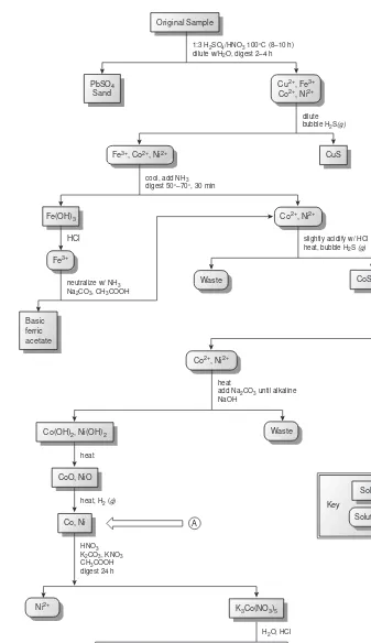
Another distinction between analytical chemistry and chemical analysis is that analytical chemists work to improve established methods. For example, sev-eral factors complicate the quantitative analysis of Ni2+in ores, including the presence of a complex heterogeneous mixture of silicates and oxides, the low con-centration of Ni2+in ores, and the presence of other metals that may interfere in the analysis. Figure 1.1 is a schematic outline of one standard method in use dur-ing the late nineteenth century.3After dissolving a sample of the ore in a mixture of H2SO4and HNO3, trace metals that interfere with the analysis, such as Pb2+, Cu2+and Fe3+, are removed by precipitation. Any cobalt and nickel in the sample are reduced to Co and Ni, isolated by filtration and weighed (point A). After dissolving the mixed solid, Co is isolated and weighed (point B). The amount of nickel in the ore sample is determined from the difference in the masses at points A and B.
%Ni = mass point A – mass point B
Original Sample
PbSO4 Sand
Basic ferric acetate
CuS 1:3 H2SO4/HNO3 100°C (8–10 h)
dilute w/H2O, digest 2–4 h
Cu2+, Fe3+ Co2+, Ni2+
Fe3+,Co2+, Ni2+
Fe(OH)3
CoS, NiS
CuS, PbS
Co(OH)2, Ni(OH)2
CoO, NiO
cool, add NH3 digest 50°–70°, 30 min
Co2+, Ni2+
Fe3+
Waste
Waste Co2+, Ni2+
aqua regia heat, add HCl until strongly acidic bubble H2S (g)
Waste Co2+
Solid Key
Solution
H2O, HCl heat
add Na2CO3 until alkaline NaOH
K3Co(NO3)5 Ni2+
neutralize w/ NH3 Na2CO3, CH3COOH
slightly acidify w/ HCl heat, bubble H2S (g) HCl
heat
Co as above Co, Ni
heat, H2 (g)
HNO3 K2CO3, KNO3 CH3COOH digest 24 h
dilute bubble H2S(g)
A
B
Figure 1.1
The combination of determining the mass of Ni2+by difference, coupled with the need for many reactions and filtrations makes this procedure both time-consuming and difficult to perform accurately.
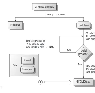
The development, in 1905, of dimethylgloxime (DMG), a reagent that selec-tively precipitates Ni2+and Pd2+, led to an improved analytical method for deter-mining Ni2+in ores.4As shown in Figure 1.2, the mass of Ni2+is measured directly, requiring fewer manipulations and less time. By the 1970s, the standard method for the analysis of Ni2+in ores progressed from precipitating Ni(DMG)
2to flame atomic absorption spectrophotometry,5 resulting in an even more rapid analysis. Current interest is directed toward using inductively coupled plasmas for determin-ing trace metals in ores.
In summary, a more appropriate description of analytical chemistry is “. . . the science of inventing and applying the concepts, principles, and . . . strategies for measuring the characteristics of chemical systems and species.”6Analytical chemists typically operate at the extreme edges of analysis, extending and improving the abil-ity of all chemists to make meaningful measurements on smaller samples, on more complex samples, on shorter time scales, and on species present at lower concentra-tions. Throughout its history, analytical chemistry has provided many of the tools and methods necessary for research in the other four traditional areas of chemistry, as well as fostering multidisciplinary research in, to name a few, medicinal chem-istry, clinical chemchem-istry, toxicology, forensic chemchem-istry, material science, geochem-istry, and environmental chemistry.
Original sample
Residue
Ni(DMG)2(s) HNO3, HCl, heat
Solution
Solid Key
Solution
20% NH4Cl 10% tartaric acid take alkaline with 1:1 NH3
Yes
No
A
take acid with HCl 1% alcoholic DMG take alkaline with 1:1 NH3 take acid with HCl
10% tartaric acid
take alkaline with 1:1 NH3 Is
solid present?
%Ni = mass A × 0.2031g sample × 100
Figure 1.2
Analytical scheme outlined by Hillebrand and
Lundell4for the gravimetric analysis of Ni in
ores (DMG = dimethylgloxime). The factor of 0.2031 in the equation for %Ni accounts for the difference in the formula weights of
Ni(DMG)2and Ni; see Chapter 8 for more
You will come across numerous examples of qualitative and quantitative meth-ods in this text, most of which are routine examples of chemical analysis. It is im-portant to remember, however, that nonroutine problems prompted analytical chemists to develop these methods. Whenever possible, we will try to place these methods in their appropriate historical context. In addition, examples of current re-search problems in analytical chemistry are scattered throughout the text.
The next time you are in the library, look through a recent issue of an analyti-cally oriented journal, such as Analytical Chemistry.Focus on the titles and abstracts of the research articles. Although you will not recognize all the terms and methods, you will begin to answer for yourself the question “What is analytical chemistry”?
1B
The Analytical Perspective
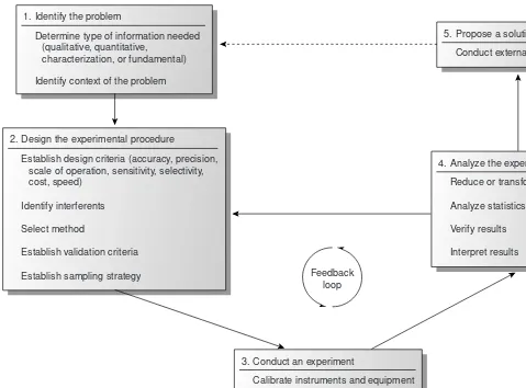
Having noted that each field of chemistry brings a unique perspective to the study of chemistry, we now ask a second deceptively simple question. What is the “analyt-ical perspective”? Many analyt“analyt-ical chemists describe this perspective as an analyt“analyt-ical approach to solving problems.7Although there are probably as many descriptions of the analytical approach as there are analytical chemists, it is convenient for our purposes to treat it as a five-step process:
1. Identify and define the problem. 2. Design the experimental procedure. 3. Conduct an experiment, and gather data. 4. Analyze the experimental data.
5. Propose a solution to the problem.
Figure 1.3 shows an outline of the analytical approach along with some im-portant considerations at each step. Three general features of this approach de-serve attention. First, steps 1 and 5 provide opportunities for analytical chemists to collaborate with individuals outside the realm of analytical chemistry. In fact, many problems on which analytical chemists work originate in other fields. Sec-ond, the analytical approach is not linear, but incorporates a “feedback loop” consisting of steps 2, 3, and 4, in which the outcome of one step may cause a reevaluation of the other two steps. Finally, the solution to one problem often suggests a new problem.
Analytical chemistry begins with a problem, examples of which include evalu-ating the amount of dust and soil ingested by children as an indicator of environ-mental exposure to particulate based pollutants, resolving contradictory evidence regarding the toxicity of perfluoro polymers during combustion, or developing rapid and sensitive detectors for chemical warfare agents.* At this point the analyti-cal approach involves a collaboration between the analytianalyti-cal chemist and the indi-viduals responsible for the problem. Together they decide what information is needed. It is also necessary for the analytical chemist to understand how the lem relates to broader research goals. The type of information needed and the prob-lem’s context are essential to designing an appropriate experimental procedure.
Designing an experimental procedure involves selecting an appropriate method of analysis based on established criteria, such as accuracy, precision, sensitivity, and detection limit; the urgency with which results are needed; the cost of a single analy-sis; the number of samples to be analyzed; and the amount of sample available for
Figure 1.3
Flow diagram for the analytical approach to
solving problems; modified after Atkinson.7c
analysis. Finding an appropriate balance between these parameters is frequently complicated by their interdependence. For example, improving the precision of an analysis may require a larger sample. Consideration is also given to collecting, stor-ing, and preparing samples, and to whether chemical or physical interferences will affect the analysis. Finally, a good experimental procedure may still yield useless in-formation if there is no method for validating the results.
The most visible part of the analytical approach occurs in the laboratory. As part of the validation process, appropriate chemical or physical standards are used to calibrate any equipment being used and any solutions whose concentrations must be known. The selected samples are then analyzed and the raw data recorded.
The raw data collected during the experiment are then analyzed. Frequently the data must be reduced or transformed to a more readily analyzable form. A statistical treatment of the data is used to evaluate the accuracy and precision of the analysis and to validate the procedure. These results are compared with the criteria estab-lished during the design of the experiment, and then the design is reconsidered, ad-ditional experimental trials are run, or a solution to the problem is proposed. When a solution is proposed, the results are subject to an external evaluation that may re-sult in a new problem and the beginning of a new analytical cycle.
1. Identify the problem
Determine type of information needed (qualitative, quantitative,
characterization, or fundamental)
Identify context of the problem
2. Design the experimental procedure
Establish design criteria (accuracy, precision, scale of operation, sensitivity, selectivity, cost, speed)
Identify interferents
Select method
Establish validation criteria
Establish sampling strategy Feedback
loop
3. Conduct an experiment
Calibrate instruments and equipment
Standardize reagents
Gather data
4. Analyze the experimental data Reduce or transform data
Analyze statistics
Verify results
Interpret results 5. Propose a solution
As an exercise, let’s adapt this model of the analytical approach to a real prob-lem. For our example, we will use the determination of the sources of airborne pol-lutant particles. A description of the problem can be found in the following article:
“Tracing Aerosol Pollutants with Rare Earth Isotopes” by Ondov, J. M.; Kelly, W. R. Anal. Chem.1991,63,691A–697A.
Before continuing, take some time to read the article, locating the discussions per-taining to each of the five steps outlined in Figure 1.3. In addition, consider the fol-lowing questions:
1. What is the analytical problem?
2. What type of information is needed to solve the problem? 3. How will the solution to this problem be used?
4. What criteria were considered in designing the experimental procedure? 5. Were there any potential interferences that had to be eliminated? If so, how
were they treated?
6. Is there a plan for validating the experimental method? 7. How were the samples collected?
8. Is there evidence that steps 2, 3, and 4 of the analytical approach are repeated more than once?
9. Was there a successful conclusion to the problem?
According to our model, the analytical approach begins with a problem. The motivation for this research was to develop a method for monitoring the transport of solid aerosol particulates following their release from a high-temperature com-bustion source. Because these particulates contain significant concentrations of toxic heavy metals and carcinogenic organic compounds, they represent a signifi-cant environmental hazard.
An aerosol is a suspension of either a solid or a liquid in a gas. Fog, for exam-ple, is a suspension of small liquid water droplets in air, and smoke is a suspension of small solid particulates in combustion gases. In both cases the liquid or solid par-ticulates must be small enough to remain suspended in the gas for an extended time. Solid aerosol particulates, which are the focus of this problem, usually have micrometer or submicrometer diameters. Over time, solid particulates settle out from the gas, falling to the Earth’s surface as dry deposition.
Existing methods for monitoring the transport of gases were inadequate for studying aerosols. To solve the problem, qualitative and quantitative information were needed to determine the sources of pollutants and their net contribution to the total dry deposition at a given location. Eventually the methods developed in this study could be used to evaluate models that estimate the contributions of point sources of pollution to the level of pollution at designated locations.
![Figure 2.1Graph of [H+] versus volume of NaOH andpH versus volume of NaOH for the reactionof 0.10 M HCl with 0.10 M NaOH.](https://thumb-ap.123doks.com/thumbv2/123dok/3556011.1779921/36.648.192.428.59.269/figure-graph-versus-volume-naoh-versus-volume-reactionof.webp)