a valuable introduction; experienced developers will find it an invaluable reference. Everything is here, from the detailed numeric issues of IEEE floating point notation, to the correct way to use quaternions and spherical linear interpolation to represent orientation, to the mathematics of collision detection and rigid-body dynamics.
—David Luebke, University of Virginia, co-author ofLevel of Detail for 3D Graphics When it comes to software development for games or virtual reality, you cannot escape the math-ematics. The best performance comes not from superfast processors and terabytes of memory, but from well-chosen algorithms. With this in mind, the techniques most useful for developing production-quality computer graphics for Hollywood blockbusters are not the best choice for interactive applications. When rendering times are measured in milliseconds rather than hours, you need an entirely different perspective.
Essential Mathematics for Games and Interactive Applications provides this perspective. While the mathematics are rigorous and perhaps challenging at times, Van Verth and Bishop provide the context for understanding the algorithms and data structures needed to bring games and VR applications to life. This may not be the only book you will ever need for games and VR software development, but it will certainly provide an excellent framework for developing robust and fast applications.
—Ian Ashdown, President, ByHeart Consultants Limited
WithEssential Mathematics for Games and Interactive Applications,Van Verth and Bishop have provided invaluable assistance for professional game developers looking to shore up weaknesses in their mathematical training. Even if you never intend to write a renderer or tune a physics engine, this book provides the mathematical and conceptual grounding needed to understand many of the key concepts in rendering, simulation, and animation.
—Dave Weinstein, Microsoft, Red Storm Entertainment
Geometry, trigonometry, linear algebra, and calculus are all essential tools for 3D graphics. Math-ematics courses in these subjects cover too much ground, while at the same time glossing over the bread-and-butter essentials for 3D graphics programmers. InEssential Mathematics for Games and Interactive Applications,Van Verth and Bishop bring just the right level of mathematics out of the trenches of professional game development. This book provides an accessible and solid mathematical foundation for interactive graphics programmers. If you are working in the area of 3D games, this book is a “must have.”
—Jonathan Cohen, Department of Computer Science, Johns Hopkins University, co-author ofLevel of Detail for 3D Graphics It’s the book with all the math you need for games.
—Neil Kirby, Bell Labs
As games become ever more sophisticated, mathematics and technical programming skills become increasingly important to have in your toolbox.Essential Mathprovides a solid foun-dation in many critical areas. You will find many topics covered in detail: from linear algebra to calculus, from physics to rasterization. Some of this will be review material, but you will undoubtedly learn something new and, most importantly, something useful.
for Games and
Interactive Applications
A Programmer’s Guide
for Games and
Interactive Applications
A Programmer’s Guide
Second Edition
James M. Van Verth
Lars M. Bishop
AMSTERDAM•BOSTON•HEIDELBERG•LONDON NEW YORK•OXFORD•PARIS•SAN DIEGO SAN FRANCISCO•SINGAPORE•SYDNEY•TOKYO
Senior Production Manager Paul Gottehrer
Cover Designer Joanne Blank
Composition diacriTech
Interior printer RR Donnelley
Cover printer Phoenix Color
Morgan Kaufmann Publishers is an imprint of Elsevier. 30 Corporate Drive, Suite 400, Burlington, MA 01803, USA This book is printed on acid-free paper.
∞Copyright © 2008 by Elsevier Inc. All rights reserved.
Designations used by companies to distinguish their products are often claimed as trademarks or registered trademarks. In all instances in which Morgan Kaufmann Publishers is aware of a claim, the product names appear in initial capital or all capital letters. Readers, however, should contact the appropriate companies for more complete information regarding trademarks and registration.
No part of this publication may be reproduced, stored in a retrieval system, or transmitted in any form or by any means—electronic, mechanical, photocopying, scanning, or otherwise—without prior written permission of the publisher. Permissions may be sought directly from Elsevier’s Science & Technology Rights Department in Oxford, UK: phone: (+44) 1865 843830, fax: (+44) 1865 853333, E-mail: [email protected]. You may also complete your request online via the Elsevier homepage (http://elsevier.com), by selecting “Support & Contact” then “Copyright and Permission” and then “Obtaining Permissions.”
Library of Congress Cataloging-in-Publication Data
APPLICATIONS SUBMITTED ISBN: 978-0-12-374297-1
ISBN: 978-0-12-374298-8 (CD-ROM)
For information on all Morgan Kaufmann publications, visit our Web site atwww.mkp.comorwww.books.elsevier.com
To Mur and Fiona, for allowing me to slay the monster one more time. —Jim
James M. Van Verthis an OpenGL Software Engineer at NVIDIA, where he works on device drivers for NVIDIA GPUs. Prior to that, he was a found-ing member of Red Storm Entertainment, where he was a lead engineer for eight years. For the past nine years he also has been a regular speaker at the Game Developers Conference, teaching the all-day tutorials “Math for Game Programmers” and “Physics for Game Programmers,” on which this book is based. His background includes a B.A. in Math/Computer Science from Dartmouth College, an M.S. in Computer Science from the State University of New York at Buffalo, and an M.S. in Computer Science from the University of North Carolina at Chapel Hill.
Preface
xixIntroduction
xxiiiChapter
1
Real-World Computer Number Representation
11.1
Introduction 11.2
Representing Real Numbers 21.2.1 Approximations 2
1.2.2 Precision and Error 3
1.3
Floating-Point Numbers 41.3.1 Review: Scientific Notation 4
1.3.2 A Restricted Scientific Notation 5
1.4
Binary “Scientific Notation” 61.5
IEEE 754 Floating-Point Standard 91.5.1 Basic Representation 9
1.5.2 Range and Precision 11
1.5.3 Arithmetic Operations 13
1.5.4 Special Values 16
1.5.5 Very Small Values 19
1.5.6 Catastrophic Cancelation 22
1.5.7 Double Precision 24
1.6
Real-World Floating-Point 251.6.1 Internal FPU Precision 25
1.6.2 Performance 26
1.6.3 IEEE Specification Compliance 29
1.6.4 Graphics Processing Units and Half-Precision Floating-Point Formats 31
1.7
Code 321.8
Chapter Summary 33Chapter
2
Vectors and Points
352.1
Introduction 352.2
Vectors 362.2.1 Geometric Vectors 36
2.2.2 Linear Combinations 39
2.2.3 Vector Representation 40
2.2.4 Basic Vector Class Implementation 42
2.2.5 Vector Length 44
2.2.6 Dot Product 47
2.2.7 Gram-Schmidt Orthogonalization 51
2.2.8 Cross Product 53
2.2.9 Triple Products 56
2.2.10 Real Vector Spaces 59
2.2.11 Basis Vectors 62
2.3
Points 632.3.1 Points as Geometry 64
2.3.2 Affine Spaces 66
2.3.3 Affine Combinations 68
2.3.4 Point Implementation 70
2.3.5 Polar and Spherical Coordinates 72
2.4
Lines 752.4.1 Definition 75
2.4.2 Parameterized Lines 76
2.4.3 Generalized Line Equation 77
2.4.4 Collinear Points 79
2.5
Planes 802.5.1 Parameterized Planes 80
2.5.2 Generalized Plane Equation 80
2.5.3 Coplanar Points 82
2.6
Polygons and Triangles 822.7
Chapter Summary 86Chapter
3
Matrices and Linear Transformations
873.1
Introduction 873.2
Matrices 883.2.1 Introduction to Matrices 88
3.2.2 Simple Operations 90
3.2.3 Vector Representation 92
3.2.4 Block Matrices 92
3.2.5 Matrix Product 94
3.2.7 Performing Vector Operations with Matrices 97
3.2.8 Implementation 98
3.3
Linear Transformations 1013.3.1 Definitions 101
3.3.2 Null Space and Range 103
3.3.3 Linear Transformations and Basis Vectors 104
3.3.4 Matrices and Linear Transformations 106
3.3.5 Combining Linear Transformations 108
3.4
Systems of Linear Equations 1103.4.1 Definition 110
3.4.2 Solving Linear Systems 112
3.4.3 Gaussian Elimination 113
3.5
Matrix Inverse 1173.5.1 Definition 117
3.5.2 Simple Inverses 120
3.6
Determinant 1213.6.1 Definition 121
3.6.2 Computing the Determinant 123
3.6.3 Determinants and Elementary Row Operations 126
3.6.4 Adjoint Matrix and Inverse 128
3.7
Eigenvalues and Eigenvectors 1293.8
Chapter Summary 130Chapter
4
Affine Transformations
1334.1
Introduction 1334.2
Affine Transformations 1344.2.1 Matrix Definition 134
4.2.2 Formal Definition 136
4.2.3 Formal Representation 138
4.3
Standard Affine Transformations 1394.3.1 Translation 139
4.3.2 Rotation 141
4.3.3 Scaling 150
4.3.4 Reflection 151
4.3.5 Shear 154
4.3.6 Applying an Affine Transformation Around an
Arbitrary Point 156
4.3.7 Transforming Plane Normals 158
4.4
Using Affine Transformations 1594.4.1 Manipulation of Game Objects 159
4.4.2 Matrix Decomposition 164
4.5
Object Hierarchies 1694.6
Chapter Summary 171Chapter
5
Orientation Representation
1735.1
Introduction 1735.2
Rotation Matrices 1745.3
Fixed and Euler Angles 1745.3.1 Definition 174
5.3.2 Format Conversion 177
5.3.3 Concatenation 178
5.3.4 Vector Rotation 178
5.3.5 Other Issues 179
5.4
Axis–Angle Representation 1815.4.1 Definition 181
5.4.2 Format Conversion 182
5.4.3 Concatenation 184
5.4.4 Vector Rotation 184
5.4.5 Axis–Angle Summary 185
5.5
Quaternions 1855.5.1 Definition 185
5.5.2 Quaternions as Rotations 186
5.5.3 Addition and Scalar Multiplication 187
5.5.4 Negation 188
5.5.5 Magnitude and Normalization 188
5.5.6 Dot Product 189
5.5.7 Format Conversion 189
5.5.8 Concatenation 193
5.5.9 Identity and Inverse 195
5.5.10 Vector Rotation 197
5.5.11 Shortest Path of Rotation 199
5.5.12 Quaternions and Transformations 200
5.6
Chapter Summary 201Chapter
6
Viewing and Projection
2036.1
Introduction 2036.2
View Frame and View Transformation 2056.2.1 Defining a Virtual Camera 205
6.2.2 Constructing the View-to-World Transformation 206
6.2.3 Controlling the Camera 208
6.3
Projective Transformation 2126.3.1 Definition 212
6.3.2 Normalized Device Coordinates 216
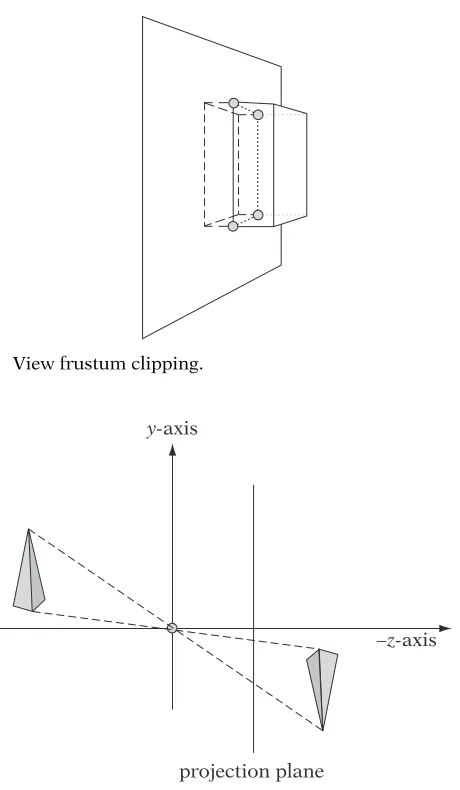
6.3.3 View Frustum 216
6.3.4 Homogeneous Coordinates 220
6.3.5 Perspective Projection 221
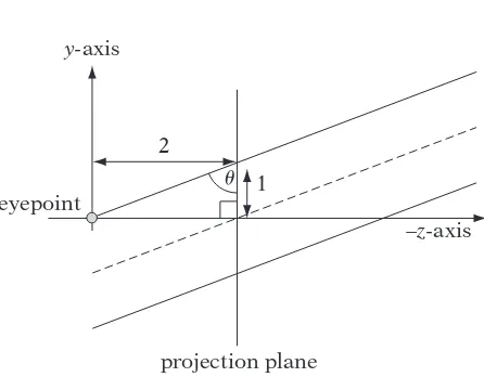
6.3.6 Oblique Perspective 228
6.3.7 Orthographic Parallel Projection 231
6.3.8 Oblique Parallel Projection 232
6.4
Culling and Clipping 2356.4.1 Why Cull or Clip? 235
6.4.2 Culling 238
6.4.3 General Plane Clipping 239
6.4.4 Homogeneous Clipping 244
6.5
Screen Transformation 2466.5.1 Pixel Aspect Ratio 248
6.6
Picking 2496.7
Management of Viewing Transformations 2526.8
Chapter Summary 254Chapter
7
Geometry and Programmable Shading
2557.1
Introduction 2557.2
Color Representation 2577.2.1 RGB Color Model 257
7.2.2 Colors as “Vectors” 257
7.2.3 Color Range Limitation 258
7.2.4 Operations on Colors 259
7.2.5 Alpha Values 260
7.2.6 Color Storage Formats 264
7.3
Points and Vertices 2667.3.1 Per-Vertex Attributes 266
7.3.2 An Object’s Vertices 267
7.4
Surface Representation 2707.4.1 Vertices and Surface Ambiguity 270
7.4.2 Triangles 271
7.4.3 Connecting Vertices into Triangles 271
7.4.4 Drawing Geometry 274
7.5
Rendering Pipeline 2757.5.1 Fixed-Function versus Programmable Pipelines 277
7.6
Shaders 2787.6.2 Shader Input and Output Values 279
7.6.3 Shader Operations and Language Constructs 280
7.7
Vertex Shaders 2807.7.1 Vertex Shader Inputs 280
7.7.2 Vertex Shader Outputs 281
7.7.3 Basic Vertex Shaders 282
7.7.4 Linking Vertex and Fragment Shaders 282
7.8
Fragment Shaders 2837.8.1 Fragment Shader Inputs 283
7.8.2 Fragment Shader Outputs 284
7.8.3 Compiling, Linking, and Using Shaders 284
7.8.4 Setting Uniform Values 286
7.9
Basic Coloring Methods 2877.9.1 Per-Object Colors 288
7.9.2 Per-Vertex Colors 288
7.9.3 Per-Triangle Colors 290
7.9.4 Sharp Edges and Vertex Colors 290
7.9.5 More about Basic Shading 291
7.9.6 Limitations of Basic Shading Methods 292
7.10
Texture Mapping 2927.10.1 Introduction 292
7.10.2 Shading via Image Lookup 293
7.10.3 Texture Images 294
7.10.4 Texture Samplers 297
7.11
Texture Coordinates 2977.11.1 Mapping Texture Coordinates onto Objects 298
7.11.2 Generating Texture Coordinates 300
7.11.3 Texture Coordinate Discontinuities 301
7.11.4 Mapping Outside the Unit Square 302
7.11.5 Texture Samplers in Shader Code 309
7.12
The Steps of Texturing 3097.12.1 Other Forms of Texture Coordinates 310
7.12.2 From Texture Coordinates to a Texture Sample Color 311
7.13
Limitations of Static Shading 3127.14
Chapter Summary 313Chapter
8
Lighting
3158.1
Introduction 3158.2
Basics of Light Approximation 3168.2.1 Measuring Light 317
8.2.2 Light as a Ray 318
8.4
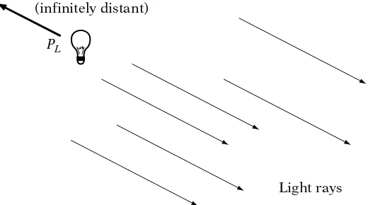
Types of Light Sources 3198.4.1 Directional Lights 320
8.4.2 Point Lights 321
8.4.3 Spotlights 327
8.4.4 Other Types of Light Sources 330
8.5
Surface Materials and Light Interaction 3318.6
Categories of Light 3328.6.1 Emission 332
8.6.2 Ambient 332
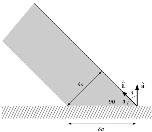
8.6.3 Diffuse 334
8.6.4 Specular 338
8.7
Combined Lighting Equation 3438.8
Lighting and Shading 3488.8.1 Flat-Shaded Lighting 349
8.8.2 Per-Vertex Lighting 350
8.8.3 Per-Fragment Lighting 354
8.9
Textures and Lighting 3588.9.1 Basic Modulation 359
8.9.2 Specular Lighting and Textures 360
8.9.3 Textures as Materials 362
8.10
Advanced Lighting 3638.10.1 Normal Mapping 363
8.11
Reflective Objects 3668.12
Shadows 3678.13
Chapter Summary 368Chapter
9
Rasterization
3699.1
Introduction 3699.2
Displays and Framebuffers 3709.3
Conceptual Rasterization Pipeline 3719.3.1 Rasterization Stages 372
9.4
Determining the Fragments: Pixels Covered by a Triangle 3739.4.1 Fragments 373
9.4.2 Depth Complexity 373
9.4.3 Converting Triangles to Fragments 375
9.4.4 Handling Partial Fragments 376
9.5
Determining Visible Geometry 3789.5.1 Depth Buffering 378
9.5.2 Depth Buffering in Practice 387
9.6
Computing Fragment Shader Inputs 3889.6.1 Uniform Values 389
9.6.3 Interpolating Texture Coordinates 392
9.6.4 Other Sources of Texture Coordinates 394
9.7
Evaluating the Fragment Shader 3959.8
Rasterizing Textures 3959.8.1 Texture Coordinate Review 396
9.8.2 Mapping a Coordinate to a Texel 396
9.8.3 Mipmapping 404
9.9
From Fragments to Pixels 4159.9.1 Pixel Blending 416
9.9.2 Antialiasing 420
9.9.3 Antialiasing in Practice 427
9.10
Chapter Summary 428Chapter
10
Interpolation
43110.1
Introduction 43110.2
Interpolation of Position 43310.2.1 General Definitions 433
10.2.2 Linear Interpolation 435
10.2.3 Hermite Curves 438
10.2.4 Catmull-Rom Splines 448
10.2.5 Kochanek-Bartels Splines 450
10.2.6 Bézier Curves 452
10.2.7 Other Curve Types 456
10.3
Interpolation of Orientation 45810.3.1 General Discussion 458
10.3.2 Linear Interpolation 461
10.3.3 Spherical Linear Interpolation 465
10.3.4 Performance Improvements 469
10.4
Sampling Curves 47010.4.1 Forward Differencing 471
10.4.2 Midpoint Subdivision 473
10.4.3 Computing Arc Length 476
10.5
Controlling Speed along a Curve 48010.5.1 Moving at Constant Speed 480
10.5.2 Moving at Variable Speed 485
10.6
Camera Control 48810.7
Chapter Summary 491Chapter
11
Random Numbers
49311.2
Probability 49311.2.1 Basic Probability 494
11.2.2 Random Variables 497
11.2.3 Mean and Standard Deviation 501
11.2.4 Special Probability Distributions 502
11.3
Determining Randomness 50511.3.1 Chi-Square Test 506
11.3.2 Spectral Test 512
11.4
Random Number Generators 51311.4.1 Linear Congruential Methods 516
11.4.2 Lagged Fibonacci Methods 520
11.4.3 Carry Methods 521
11.4.4 Mersenne Twister 523
11.4.5 Conclusions 526
11.5
Special Applications 52711.5.1 Integers and Ranges of Integers 527
11.5.2 Floating-Point Numbers 528
11.5.3 Nonuniform Distributions 528
11.5.4 Spherical Sampling 530
11.5.5 Disc Sampling 532
11.5.6 Noise and Turbulence 534
11.6
Chapter Summary 538Chapter
12
Intersection Testing
54112.1
Introduction 54112.2
Closest Point and Distance Tests 54212.2.1 Closest Point on Line to Point 542
12.2.2 Line–Point Distance 544
12.2.3 Closest Point on Line Segment to Point 545
12.2.4 Line Segment–Point Distance 546
12.2.5 Closest Points Between Two Lines 548
12.2.6 Line–Line Distance 550
12.2.7 Closest Points Between Two Line Segments 551
12.2.8 Line Segment–Line Segment Distance 553
12.2.9 General Linear Components 554
12.3
Object Intersection 55412.3.1 Spheres 556
12.3.2 Axis-Aligned Bounding Boxes 563
12.3.3 Swept Spheres 571
12.3.4 Object-Oriented Boxes 576
12.4
A Simple Collision System 58812.4.1 Choosing a Base Primitive 589
12.4.2 Bounding Hierarchies 590
12.4.3 Dynamic Objects 591
12.4.4 Performance Improvements 593
12.4.5 Related Systems 596
12.4.6 Section Summary 599
12.5
Chapter Summary 599Chapter
13
Rigid Body Dynamics
60113.1
Introduction 60113.2
Linear Dynamics 60213.2.1 Moving with Constant Acceleration 602
13.2.2 Forces 605
13.2.3 Linear Momentum 606
13.2.4 Moving with Variable Acceleration 607
13.3
Numerical Integration 60913.3.1 Definition 609
13.3.2 Euler’s Method 611
13.3.3 Runge-Kutta Methods 614
13.3.4 Verlet Integration 616
13.3.5 Implicit Methods 619
13.3.6 Semi-Implicit Methods 621
13.4
Rotational Dynamics 62213.4.1 Definition 622
13.4.2 Orientation and Angular Velocity 622
13.4.3 Torque 625
13.4.4 Angular Momentum and Inertia Tensor 626
13.4.5 Integrating Rotational Quantities 628
13.5
Collision Response 63013.5.1 Contact Generation 630
13.5.2 Linear Collision Response 634
13.5.3 Rotational Collision Response 638
13.5.4 Extending the System 640
13.6
Efficiency 64313.7
Chapter Summary 645Bibliography
647Index
655Trademarks
671Writing a book is an adventure. To begin with, it is a toy and an amusement; then it becomes a mistress, and then it becomes a master, and then a tyrant. The last phase is that just as you are about to be reconciled to your servitude, you kill the monster, and fling him out to the public. — Sir Winston Churchill
The Adventure Begins
As humorous as Churchill’s statement is, there is a certain amount of truth to it; writing this book was indeed an adventure. There is something about the process of writing, particularly a nonfiction work like this, that forces you to test and expand the limits of your knowledge. We hope that you, the reader, benefit from our hard work.
How does a book like this come about? Many of Churchill’s books began with his experience — particularly his experience as a world leader in wartime. This book had a more mundane beginning: Two engineers at Red Storm Entertainment, separately, asked Jim to teach them about vectors. These engineers were 2D game programmers, and 3D was not new, but was starting to replace 2D at that point. Jim’s project was in a crunch period, so he didn’t have time to do much about it until proposals were requested for the annual Game Developers Conference. Remembering the engineers’ request, he thought back to the classic “Math for SIGGRAPH” course from SIGGRAPH 1989, which he had attended and enjoyed. Jim figured that a similar course, at that time titled “Math for Game Programmers,” could help 2D programmers become 3D programmers.
The course was accepted, and together with a co-speaker, Marcus Nordenstam, Jim presented it at GDC 2000. The following years (2001–2002) Jim taught the course alone, as Marcus had moved from the game industry to the film industry. The sub-ject matter changed slightly as well, adding more advanced material such as curves, collision detection, and basic physical simulation.
It was in 2002 that the seeds of what you hold in your hand were truly planted. At GDC 2002, another GDC speaker, whose name, alas, is lost to time, recommended that Jim turn his course into a book. This was an interesting idea, but how to get it published? As it happened, Jim ran into Dave Eberly at SIGGRAPH 2002, and he was looking for someone to write just that book for Morgan Kaufmann. At the same time, Lars, who was working at Numeric Design Limited at the time, was presenting some
of the basics of rendering on handheld devices as part of a SIGGRAPH course. Jim and Lars discussed the fact that handheld 3D rendering had brought back some of the “lost arts” of 3D programming, and that this might be included in a book on mathematics for game programming.
Thus, a co-authorship was formed. Lars joined Jim in teaching the GDC 2003 version of what was now called “Essential Math for Game Programmers,” and simul-taneously joined Jim to help with the book, helping to expand the topics covered to include numerical representations. As we began to flesh out the latter chapters of the outline, Lars was finding that the advent of programmable shaders on consumer 3D hardware was bringing more and more low-level lighting, shading, and texturing ques-tions into his office at NDL. Accordingly, the planned single chapter on “texturing and antialiasing” became three, covering a wider selection of these rendering topics.
By early 2003, we were furiously typing the first full draft of the first edition of this book, and by GDC 2004 the book was out. Having defeated the dragon, we retired to our homes to live out the rest of our quiet little lives.
Or so we thought.
The Adventure Continues
Response to the first edition was quite positive, and the book continued to sell well beyond the initial release. Naturally, thoughts turned to what we could do to improve the book beyond what we already created.
In reviewing the topic list, it was obvious what the most necessary change was. Within a year or so of the publication of the first edition, programmable shading had revolutionized the creation of 3D applications on game consoles and on PC. While the first edition had provided readers with many of the fundamentals behind the mathe-matics used in shaders, it stopped short of actually discussing them in detail. It was clear that the second edition needed to embrace shaders completely, applying the mathematics of the earlier chapters to an entirely new set of rendering content. So the single biggest change in the second edition is a move to a purely shader-based rendering pipeline.
We also sent the book to reviewers to ask them what they would like to see added. The two most common requests were information about random numbers and the addition of problems and exercises. So we are providing both. A brand new chapter on probability and random numbers has been added, and problems and exercises for each chapter have been added to the CD in the back of the book. In addition, the entire book has been revised to add corrections and make the content flow better. We hope you’ll find our efforts worthwhile.
Both times, the experience was fascinating, sometimes frustrating, but ultimately deeply rewarding. Hopefully, this fascination and respect for the material will be con-veyed to you, the reader. The topics in this book can each take a lifetime to study to a truly great depth; we hope you will be convinced to try just that, nonetheless!
system goes wrong (and italwaysdoes), the best programmers are never satisfied with “I fixed it, but I’m not sure how;” without understanding, there can be no confidence in the solution, and nothing new is learned. Such programmers are driven by the desire to understand what went wrong, how to fix it, and learning from the experience. No other tool in 3D programming is quite as important to this process than the mathematical bases1behind it.
Those Who Helped Us Along the Road
In a traditional adventure the protagonists are assisted by various characters that pass in and out of the pages. Similarly, while this book bears the names of two people on the cover, the material between its covers bears the mark of many, many more. We would like to thank a few of them here.
The folks at our publisher, Elsevier, were extremely patient with both of us as we made up for being more experienced this time around by being more busy and less responsive! Chris Simpson, Laura Lewin, Georgia Kennedy, and Paul Gottehrer were all patient, professional, and flexible when we most needed it.
In addition, credit is still due to the folks at Morgan Kaufmann who helped us publish the first edition. Tim Cox, our editor, and Stacie Pierce and Richard Camp, his assistants, as well as Troy Lilly (in production) were patient and helpful in the daunting task of leading two first-time authors through the process. Special thanks are due to Dave Eberly, the series editor of our first edition, who read most of the book several times and provided great encouragement (and the occasional scolding) through the entire process, one he’s been through firsthand several times.
Our reviewers were top-notch. Together, Erin Catto and Chad Robertson reviewed the entire second edition of the book. Robert Brown, Matthew McCallus, Greg Stel-mack, and Melinda Theilbar were invaluable for their comments on the random numbers chapter. Ian Ashdown, Steven Woodcock, John O’Brien, J.R. Parker, Neil Kirby, John Funge, Michael van Lent, Peter Norvig, Tomas Akenine-Möller, Wes Hunt, Peter Lipson, Jon McAllister, Travis Young, Clark Gibson, Joe Sauder, and Chris Stoy each reviewed parts of the first edition or the proposals for them. Despite having tight deadlines, they all provided page after page of useful feedback, keeping us honest and helping us generate a better arc to the material. Several of them wentwellabove and beyond the call of duty, providing detailed comments and even re-reading sections of the book that required significant changes. Finally, thanks also to Victor Brueggemann and Garner Halloran, who asked Jim the questions that started this whole thing off five years ago.
Jim and Lars would like to acknowledge the folks at their jobs at NVIDIA Corpo-ration, who wereveryunderstanding with respect to the time-consuming process of creating a book. Also, thanks to the talented engineers at this and previous companies who provided the probing discussions and great questions that led to and continually fed this book.
In addition, Jim would like to thank Mur and Fiona, his wife and daughter, who were willing to put up with this a second time after his long absences the first time through; his sister, Liz, who provided illustrations for an early draft of this text; and his parents, Jim and Pat, who gave him the resources to make it in the world and introduced him to the world of computers so long ago.
Lars would like to thank Jen, his wife, who somehow had the courage to survive a second edition of the book even after being promised that the first edition “was it;” and his parents, Steve and Helene, who supported, nutured, and taught him so much about the value of constant learning and steadfast love.
The (Continued) Rise of 3D Games
Over the past decade or so (driven by increasingly powerful computer and video game console hardware), three-dimensional (3D) games have expanded from custom-hardware arcade machines to the realm of hardcore PC games, to consumer set-top video game consoles, and even to handheld devices such as personal digital assistants (PDAs) and cellular telephones. This explosion in popularity has lead to a corre-sponding need for programmers with the ability to program these games. As a result, programmers are entering the field of 3D games and graphics by teaching themselves the basics, rather than a classic college-level graphics and mathematics education. At the same time, many college students are looking to move directly from school into the industry. These different groups of programmers each have their own set of skills and needs in order to make the transition. While every programmer’s situation is different, we describe here some of the more common situations.
Many existing, self-taught 3D game programmers have strong game experi-ence and an excellent practical approach to programming, stressing visual results and strong optimization skills that can be lacking in college-level computer science programs. However, these programmers are sometimes less comfortable with the conceptual mathematics that form the underlying basis of 3D graphics and games. This can make developing, debugging, and optimizing these systems more of a trial-and-error exercise than would be desired.
Programmers who are already established in other specializations in the game industry, such as networking or user interfaces, are now finding that they want to expand their abilities into core 3D programming. While having experience with a wide range of game concepts, these programmers often need to learn or refresh the basic mathematics behind 3D games before continuing on to learn the applications of the principles of rendering and animation.
On the other hand, college students entering (or hoping to enter) the 3D games industry often ask what material they need to know in order to be prepared to work on these games. Younger students often ask what courses they should attend in order to gain the most useful background for a programmer in the industry. Recent graduates, on the other hand, often ask how their computer graphics knowledge best relates to the way games are developed for today’s computers and game consoles.
We have designed this book to provide something for each of these groups of readers. We attempt to provide readers with a conceptual understanding of the
mathematics needed to create 3D games, as well as an understanding of how these mathematical bases actuallyapplyto games and graphics. The book provides not only theoretical mathematical background, but also many examples of how these concepts are used to affect how a game looks (how it isrendered) and plays (how objects move and react to users). Each type of reader is likely to find sections of the book that, for them, provide mainly refresher courses, a new understanding of the applications of basic mathematical concepts, or even completely new information. The specific sec-tions that fall into each category for a particular reader will, of course, depend on the reader.
How to Read This Book
Perhaps the best way to discuss any reader’s approach to reading this book is to think in terms of how a 3D game or other interactive application works at the highest level. Most readers of this book likely intend to apply what they learn from it to create, extend, or fix a 3D game or other 3D application. Each chapter in this book deals with a different topic that has applicability to some or all of the major parts of a 3D game.
Game Engines
An interactive 3D application such as a game requires quite a large amount of code to do all of the many things asked of it. This includes representing the virtual world, animating parts of it, drawing that virtual world, and dealing with user interaction in a game-relevant manner. The bulk of the code required to implement these features is generally known as agame engine. Game engines have evolved from small, simple, low-level rendering systems in the early 1990s to massive and complex software systems in modern games, capable of rendering detailed and expansive worlds, animating realistic characters, and simulating complex physics. At their core, these game engines are really implementations of the concepts discussed throughout this book.
Initially, game engines were custom affairs, written for a single use as a part of the game itself, and thrown away after being used for that single game project. Today, game developers have several options when considering an engine. They may pur-chase a commercial engine from another company and use it unmodified for their project. They may purchase an engine and modify it very heavily to customize their application. Finally, they may write their own, although most programmers choose to use such an internally developed engine for multiple games to offset the large cost of creating the engine.
In any of these cases, the developer must still understand the basic concepts of the game engine. Whether as a user, a modifier, or an author of a game engine, the developer must understand at least a majority of the concepts presented in this book. To better understand how the various chapters in this book surface in game engines, we first present a commonmain loopas it might appear in a game engine:
1. Draw the current configuration of the game’s scene to the screen.
3. Detect collisions between the characters and objects (e.g., the soccer ball entering the goal or two players sliding into one another).
4. React to these collisions and basic forces such as gravity in the scene in a physically correct manner (e.g., the soccer ball in flight).
All of these steps will need to be done for each frame to present the player with a convincing game experience. Thus, the code to implement the steps above must be correct and optimal.
Chapters 1–5: The Basics
Perhaps the most core parts of any game engine are the low-level mathematical and geometric representations and algorithms. The pieces of code will be used by each and every step listed above. Chapter 1 provides the lowest-level basis for this. It discusses the practicalities of representing real numbers on a computer, with a focus on the issues most likely to affect the development of a 3D game engine for a PC, console, or handheld device.
Chapter 2 provides a focused review of vectors and points, objects that are used in all game engines to represent locations, directions, velocities, and other geometric quantities in all aspects of a 3D application. Chapters 3 and 4 review the basics of linear and affine algebra as they relate to orienting, moving, and distorting the objects and spaces that make up a virtual world. Finally, Chapter 5 introduces the quaternion, a very powerful nonmatrix representation of object orientation that will be pivotal to the later chapters on animation and simulation.
Three-dimensional engine code that implements all of these fundamental objects must be built carefully and with a good understanding of both the underlying mathe-matics and programming issues. Otherwise, the game engine built on top of these basic objects or functions will be based upon a poor foundation. Many game programmers’ multiday debugging sessions have ended with the realization that the complex bug was rooted in an error in the engine’s basic mathematics code.
Some readers will have a passing familiarity with the topics in these chapters. However, most readers will want to start with these chapters, as many of the topics are covered in more conceptual detail than is often discussed in basic graphics texts. Readers new to the material will want to read in detail, while those who already know some linear algebra can use the chapters to fill in any missing background. All of these chapters form a basis for the rest of the book, and an understanding of these topics, whether existing or new, will be key to successful 3D programming.
Chapters 6–9: Rendering
of color and the concept ofshaders, which are short programs that allow modern graphics hardware to draw the scene objects to the display device. Chapter 8 explains how to use these programmable shaders to implement simple approximations of real-world lighting. The rendering section concludes with Chapter 9, which details the methods used by low-level rendering systems to draw to the screen. An understanding of these details can allow programmers to create much more efficient and artifact-free rendering code for their engines.
Chapters 10–13: Animation and Physics
The game engine loop’s step 2, animating characters and other objects based on data created by computer animators or motion-captured data, is introduced in Chapter 10. This chapter discusses methods for smoothly animating the position, orientation, and appearance of objects in the virtual game world. The importance of good, complex character and object animation in modern engines continues to grow as new games attempt to create smoother, more convincing representations of athletes, rock stars, soldiers, and other human characters.
Chapter 11 covers another element for adding realism to games: random num-bers. Everything up to this point has been carefully determined and planned by the programmer or artist. Adding randomness adds the unexpected behavior that we see in real life. Gunshots are not always exact, clouds are not perfectly spherical, and walls are not pristine. This chapter discusses how to handle randomness in a game, and how we can get effects such as those discussed above.
Step 3, detecting collisions, is discussed in Chapter 12. This chapter describes the mathematics and programming behind detecting when two game objects touch, inter-sect, or penetrate. Many genres of game have exacting requirements when it comes to collision, be it a racing game, a sports title, or a military simulation.
Finally, step 4, reacting in a realistic manner to physical forces and collisions, is covered in Chapter 13. This chapter describes how to make game objects behave and react in physically convincing ways.
Put together, the chapters that form this book are designed to give a good basis for the foundations of a game engine, details on the ways that engines represent and draw their virtual worlds, and an introduction to making those worlds seem real and active.
Interactive Demo Applications
Source Code
Demo
Name
to illustrate the concepts in a way that is analogous to the static figures in the book itself. Throughout the book, you will find references to interactive demos that may be found on the CD-ROM. Whenever a topic is illustrated with an interactive demo, a special icon like the one seen next to this paragraph will appear in the margin.
Support Libraries
Source Code
Library
Name
In addition to the source code for each of the demos, the CD-ROM includes the sup-porting libraries used to create the demos, with full source code. Often, code from these supporting libraries is excerpted in the book itself in order to explain how the particular concept is implemented. In such situations, an icon will appear in the mar-gin to note where the library code may be found on the CD-ROM. This source code is designed to allow readers to modify and experiment themselves, as a way of better understanding the way the code works.
The source code is written entirely in C++, a language that is likely to be familiar to most game developers. C++ was chosen because it is one of the most commonly used languages in 3D game development and because vectors, matrices, quaternions, and graphics algorithms decompose very well into C++ classes. In addition, C++’s support of operator overloading means that the math library can be implemented in a way that makes the code look very similar to the mathematical derivations in the text. However, in some sections of the text, the class declarations as printed in the book are not complete with respect to the code on the CD-ROM. Often, class members that are not relevant to the particular discussion (especially mem-ber variable accessor and “housekeeping” functions) have been omitted for clarity. These other functions may be found in the full class declarations/definitions on the CD-ROM.
Note that we have modified our mathematical notation slightly to allow our equa-tions to be as compatible as possible with the code. Mathematicians normally start indexing with 1, for example, P1, P2, . . . , Pn. This does not match how indexing is done in C++:P[0]is the first element in the arrayP. To avoid this disconnect, in our equations we will be using the convention that the starting element in a list is indexed as 0; thus,P0, P1, . . . , Pn−1. This should allow for a direct translation from equation to code.
Math Libraries
The animation demos use a shared library calledIvCurves, which includes classes that implement spline curves, the basic objects used to animate position,IvCurvesis built uponIvMath, extending this basic functionality to include animation. As with
IvMath, theIvCurveslibrary is likely to be useful beyond the scope of the book, as these classes are flexible enough to be used (along withIvMath) in other applications. Finally, the simulation demos use a shared library calledIvCollision, which implements basic object intersection (collision) data structures and algorithms. Build-ing on theIvMathlibrary, this set of classes and functions forms not only the basis for the later demos in the book, but also is an excellent starting point for experimentation with other forms of object collision and physics modeling.
Engine and Rendering Libraries
In addition to the math libraries, the CD-ROM includes a set of classes that implement a simple game like application framework, basic rendering, input handling, and timer functionality. All of these functions are grouped under the heading of game engine functionality, and are located in theIvEnginelibrary. The engine’s rendering code takes the form of a set of renderer-abstraction classes that simplify the interfaces between the C++ classes inIvMathand the C-based, low-level rendering application programmer interfaces (APIs). This code is included as a part of the rendering library
IvGraphics. It includes renderer setup, basic render-state management, and rendering of simple geometric primitives, such as spheres, cubes, and boxes.
Furthermore, a set of basic classes that implement a simple hierarchial data struc-ture called a scene graph are included in the libraryIvScene. The classes inIvScene
use and depend on the functionality of theIvCollisionlibrary. As a result, to avoid unnecessary code dependencies, the scene graph classes were placed in their own library, rather than inIvEngine.
Since this book focuses on the mathematics and concepts behind 3D games, we chose not to center the discussion around a large-scale, general 3D rendering engine. Doing so would introduce an extra layer of indirection that would not serve the concep-tual requirements of the book. Valuable real estate in the rendering chapters would be spent on background in the use of a particular engine — the one written for the book. For an example and discussion of a full, hierarchical rendering engine, the reader is encouraged to read David Eberly’s3D Game Engine Design[25].
We have opted to implement our rendering system and examples using two stan-dard SDKs: the multiplatform OpenGL [83] and the popular Direct3D DX9 [47]. We also use the utility toolkits provided with these SDKs (OpenGL’s GLUT and Direct3D’s D3DX) to implement cross-platform renderer setup and input handling, neither of which are core topics of this book.
Exercises and Supplementary Material
has an associated set of exercises, ranging from easy to hard questions, that should help those readers interested in testing their understanding of the material within. Certain chapters also have supplemental material that unfortunately didn’t make its way into the book proper due to space considerations. Those chapters have notes at their end indicating that such material is available on the CD-ROM.
References and Further Reading
Hopefully, this book will leave readers with a desire to learn even more details and the breadth of the mathematics involved in creating high-performance, high-quality 3D games. Wherever possible, we have included references to other books, articles, papers, and websites that detail particular subtopics that fall outside the scope of this book. The full set of references may be found at the back of the book.
We have attempted to include references that the vast majority of readers should be able to locate. When possible, we have referenced recent and/or standard indus-try texts and well-known conference proceedings. However, in some cases we have included references to older magazine articles and technical reports when we found those references to be particularly complete, seminal, or well written. In some cases, older references can be easier for the less-experienced reader to understand, as they often tend to assume less common knowledge when it comes to computer graphics and game topics.
In the past, older magazine articles and technical reports were notoriously difficult for the average reader to locate. However, the Internet and digital publishing have made great strides toward reversing this trend. For example, the following sources have made several classes of resources far more accessible:
■ The magazine most commonly referenced in this book,Game Developer, offers CD-ROMs that contain every issue of the magazine ever published. Copies of these CD-ROMs are available from www.gdmag.com. Several other technical magazines also offer such CD-ROMs.
■ Technical societies are now placing major historical publications into their “dig-ital libraries,” which are often made accessible to members. The Association for Computing Machinery (ACM) has done this via their ACM Digital Library, which is available to ACM members. As an example, the full text of the entire collection of papers from all SIGGRAPH conferences (the conference proceed-ings most frequently referenced in this book) is available electronically to ACM SIGGRAPH members.
1
Real-World
Computer Number
Representation
1.1
Introduction
In this chapter we’ll discuss what is perhaps the most fundamental basis upon which three-dimensional (3D) graphics pipelines are built: computer representation of numbers, particularly real numbers. While 3D programmers often use the computer representations (approximations) of real numbers suc-cessfully without any understanding of how they are implemented, this can lead to subtle bugs and performance problems at inopportune stages in the development of an application. Most basic undergraduate computer architec-ture books [106] present the basics of integral data types (e.g.,intandunsigned int,short, etc. in C/C++), but give only brief introductions to floating-point and other nonintegral number representations. Since the mathematics of 3D graphics are generally real-valued (as we shall see from the ubiquity of R, R2, andR3 in the coming chapters), it is important for anyone in the field to understand the features, limitations, and idiosyncracies of the computer representation of these nonintegral types.
In this chapter we will discuss the major computer representation of the real numbers, floating-point, along with the associated bitwise formats, basic operations, features, and limitations. By design, we will transition from general mathematical discussions of number representation toward implementation-related topics of specific relevance to 3D graphics program-mers. Most of the chapter will be spent on the ubiquitous Institute of Electrical and Electronic Engineers (IEEE) floating-point numbers, espe-cially discussions of floating-point limitations that often cause issues in
3D pipelines. A brief case study of floating-point-related performance issues in a real application is also presented.
We will assume that the reader is familiar with the basic concepts of integer and whole-number representations on modern computers, including signed representation via two’s complement, range, overflow, common stor-age lengths (8,16, and 32 bits), standard C and C++basic types (int,unsigned int,short, etc.), and type conversion. For an introduction to these concepts of binary number representation, we refer the reader to a basic computer architecture text, such as Stallings [106], and to the C++specification [30].
1.2
Representing Real Numbers
Real numbers are, to most developers, the heart and soul of a 3D graphics system. Most of the rest of the text is based upon real numbers and spaces such asR2andR3. They are the most flexible and powerful of the number rep-resentations on most computers and, not surprisingly, the most complicated and problematic. We will present the methods that are used to represent real numbers on computers today and will include numerous sections describing common issues that arise from the use of these representations in real-world applications.
The well-known issues relating to storage of integers (such as overflow) remain pertinent issues with respect to real-number representation. However, real-number representations add additional complexities that will result in implementation trade-offs, subtle errors, and difficult-to-trace performance issues that can easily confuse the programmer.
1.2.1
Approximations
While computer representations of whole numbers (unsigned int) and inte-gers (int) are limited to a finite subset of their pure counterparts, in each case the finite set is contiguous; that is, ifiandi+2are both representable, then
i+1is also representable. Inside the range defined by the minimum and max-imum representable integer values, all integers can be represented exactly. This is possible because any finitely bounded range of integers contains a finite number of elements.
When dealing with real numbers, however, this is no longer true. A subset of real numbers can have infinitely many elements even when bounded by finite minimal and maximal values. As a result, no matter how tightly we bound the range of real numbers (other than the trivial case ofRmin=Rmax)
In order to adequately understand the representations of real numbers, we need to understand the concept of precision and error.
1.2.2
Precision and Error
For any numerical representation system, we imagine a generic function
Rep(A), which returns the value in that system that is closest to the value
A. In a perfect representation system,Rep(A) =Afor all values ofA. When representing real numbers on a computer, however, even limiting range to finite extremes will not allow us to represent all numbers in the bounded range exactly. Rep(A) will be a many-to-one mapping, with infinitely many real numbersAmapping to each distinct value returned byRep(A). For each such distinctRep(A), almost all valuesAthat map to it will not be represented exactly. In other words, for almost all real valuesA,Rep(A)=A. The obvious result in such cases is that(Rep(A)−A)=0. The representation in such a case is an approximation of the actual value.
Making use of(Rep(A)−A), we can define several derived values that form metrics of the error induced by representingAin the representation system. Two such error metrics are calledabsolute errorandrelative error.
The simplest way to represent error is absolute error, which is defined as
AbsError= |Rep(A)−A|
This is simply the “number line” distance between the actual value and its representation. While this value does correctly signify the difference between the actual and representative values, it does not quantify another important factor in representation error — the scale at which the error affects computation.
To better understand this scale factor, imagine a system of measurement that is accurate to within a kilometer. Such a system might be considered suitably accurate for measuring the 149,597,871 km between Earth and the sun. However, it likely would be woefully inaccurate at measuring the size of an apple (0.00011 km), which would be rounded to 0 km! Intuitively, this is obvious, but in both cases the absolute error of representation is less than 1 km. Clearly, absolute error is not sufficient in all cases.
Relative error takes the scale of the value being approximated into account. It does so by dividing the absolute error by the actual value being represented. Relative error is defined as
RelError=
division, relative error cannot be computed for a value that approximates zero. It is a measure of the ratio of the error to the magnitude of the value being approximated. Revisiting our previous example, the relative errors in each case would be (approximately)
RelErrorSun=
1km
149,597,871km
≈7×10⁻⁹
RelErrorApple=
0.00011km
0.00011km
=1.0
Clearly, relative error is a much more useful error metric in this case. The Earth–sun distance error is tiny (compared to the distance being measured), while the size of the apple was estimated so poorly that the error had the same magnitude as the actual value. In the former case a relatively “exact” representation was found, while in the latter case the representation is all but useless.
1.3
Floating-Point Numbers
1.3.1
Review: Scientific Notation
In order to better introduce floating-point numbers, it is instructive to review the well-known standard representation for real numbers in science and engineering: scientific notation. Computer floating-point is very much analo-gous to scientific notation.
Scientific notation (in its strictest, so-called normalized form) consists of two parts:
1. A decimal number, called themantissa, such that
1.0≤ |mantissa|<10.0
2. An integer, called theexponent.
Together, the exponent and mantissa are combined to create the number
Any decimal number can be represented in this notation (other than 0, which is simply represented as 0.0), and the representation is unique for each number. In other words, for two numbers written in this form of scientific notation, the numbers are equal if and only if their mantissas and exponents are equal. This uniqueness is a result of the requirements that the exponent be an integer and that the mantissa be “normalized” (i.e., have magnitude in the range [1.0, 10.0]). Examples of numbers written in scientific notation include
102=1.02×10²
243,000=2.43×10⁵
−0.0034= −3.4×10⁻³
Examples of numbers that constitute incorrect scientific notation include
Incorrect=Correct
11.02×103=1.102×10⁴ 0.92×10−2=9.2×10⁻³
1.3.2
A Restricted Scientific Notation
For the purpose of introducing the concept of finiteness of representation, we will briefly discuss a contrived, restricted scientific notation. We extend the rules for scientific notation:
1. The mantissa must be written with a single, nonzero integral digit.
2. The mantissa must be written with a fixed number of fractional digits (we define this asMdigits).
3. The exponent must be written with a fixed number of digits (we define this asEdigits).
4. The mantissa and the exponent each have individual signs.
For example, the following number is in a format withM=3,E=2:
±1.1 2 3 ×10±1 2
there are a limited number of values that could ever be represented exactly by this system, namely:
(exponents)×(mantissas)×(exponent signs)×(mantissa signs)
=(102)×(9×103)×(2)×(2)
=3,600,000
Note that the leading digit of the mantissa must be nonzero (since the mantissa is normalized), so that there are only nine choices for its value [1, 9], leading to9×10×10×10=9,000possible mantissas.
This adds finiteness to both the range and precision of the notation. The minimum and maximum exponents are
±(10E−1)= ±(102−1)= ±99
The largest mantissa value is
10.0−(10−M)=10.0−(10−3)=10.0−0.001=9.999
Note that the smallest allowed nonzero mantissa value is still 1.000 due to the requirement for normalization. This format has the following numerical limitations:
Maximum representable value: 9.999×1099
Minimum representable value: −9.999×1099
Smallest positive value: 1.000×10−99
While one would likely never use such a restricted form of scientific notation in practice, it demonstrates the basic building blocks of binary floating-point, the most commonly used computer representation of real numbers in modern computers.
1.4
Binary “Scientific Notation”
There is no reason that scientific notation must be written in base-10. In fact, in its most basic form, the real-number representation known as floating-point is similar to a base-2 version of the restricted scientific notation given previously. In base-2, our restricted scientific notation would become
SignM×mantissa×2SignE×exponent
Mantissais a bit more complicated. It is anM+1-bit number whose most significant bit is 1. Mantissais actually a “fixed-point” number. Fixed-point numbers are based on a very simple observation with respect to computer representation of integers. In the standard binary representation, each bit represents twice the value of the bit to its right, with the least significant bit representing 1. The following diagram shows these powers of two for a standard 8-bit unsigned value:
27 26 25 24 23 22 21 20
128 64 32 16 8 4 2 1
Just as a decimal number can have a decimal point, which represents the break between integral and fractional values, a binary value can have a binary point, or more generally a radix point (a decimal number is referred to as radix 10, a binary number as radix 2). In the common integer number layout, we can imagine the radix point being to the right of the last digit. However, it does not have to be placed there. For example, let us place the radix point in the middle of the number (between the fourth and fifth bits). The diagram would then look like this:
23 22 21 20.2−1 2−2 2−3 2−4
8 4 2 1 . 12 14 18 161
Now, the least significant bit represents 1/16. The basic idea behind fixed-point is one of scaling. A fixed-fixed-point value is related to an integer with the same bit pattern by an implicit scaling factor. This scaling factor is fixed for a given fixed-point format and is the value of the least significant bit in the representation. In the case of the preceding format, the scaling factor is 1/16. The standard nomenclature for a fixed-point format is “A-dot-B,” where
defined to be 1, so the resulting fixed-pointmantissais in the range
1.0≤mantissa≤
2.0− 1
2M
Put together, the format involvesM+E+3bits (M+1for the mantissa,E
for the exponent, and two for the signs). Creating an example that is analogous to the preceding decimal case, we analyze the case ofM=3, E=2:
±1. 0 1 0×2±0 1
Any value that can be represented by this system can be represented uniquely by 8 bits. The number of values that ever could be represented exactly by this system is
(exponents)×(mantissas)×(exponent signs)×(mantissa signs)
=(22)×(1×23)×(2)×(2)
=27=128
This seems odd, as an 8-bit number should have 256 different values. However, note that the leading bit of the mantissa must be 1, since the man-tissa is normalized (and the only choices for a bit’s value are 0 and 1). This effectively fixes one of the bits and cuts the number of possible values in half. We shall see that the most common binary floating-point format takes advantage of the fact that the integral bit of the mantissa is fixed at 1.
In this case, the minimum and maximum exponents are
±(2E−1)= ±(22−1)= ±3
The largest mantissa value is
2.0−2−M =2.0−2−3=1.875
This format has the following numerical limitations: Maximum representable value: 1.875×23=15
Minimum representable value: −1.875×23= −15
Smallest positive value: 1.000×2−3=0.125
1.5
IEEE 754 Floating-Point Standard
By the early to mid-1970s, scientists and engineers were using floating-point very frequently to represent real numbers; at the time, higher-powered computers even included special hardware to accelerate floating-point calculations. However, these same scientists and engineers were finding the lack of a floating-point standard to be problematic. Their complex (and often very important) numerical simulations were producing different results, depending only on the make and model of computer upon which the simula-tion was run. Numerical code that had to run on multiple platforms became riddled with platform-specific code to deal with the differences between different floating-point processors and libraries.
In order for cross-platform numerical computing to become a reality, a standard was needed. Over the course of the next decade, a draft standard for floating-point formats and behaviors became the de facto standard on most floating-point hardware. Once adopted, it became known as the IEEE 754 floating-point standard [2], and it forms the basis of almost every hardware and software floating-point system on the market.
While the history of the standard is fascinating [62], this section will focus on explaining part of the standard itself, as well as using the standard and one of its specified formats to explain the concepts of modern floating-point arithmetic.
1.5.1
Basic Representation
The IEEE standard specifies a 32-bit “single-precision” format for floating-point numbers, as well as a 64-bit “double-precision” format. It is this single-precision format that is of greatest interest for most games and interactive applications and is thus the format that will form the basis of most of the floating-point discussion in this text. The two formats are fundamentally similar, so all of the concepts regarding single precision are applicable to double-precision values as well.
The following diagram shows the basic memory layout of the IEEE single-precision format, including the location and size of the three components of any floating-point system: sign, exponent, and mantissa:
Sign Exponent Mantissa
1 bit 8 bits 23 bits
negative exponents is handled in the exponent itself (and is discussed next). The only difference betweenXand−Xin IEEE floating-point is the high-order bit. A sign bit of 0 indicates a positive number, and a sign bit of 1 indicates a negative number.
This sign bit format allows for some efficiencies in creating a floating-point math system either in hardware or software. To negate a floating-floating-point number, simply “flip” the sign bit, leaving the rest of the bits unchanged. To compute the absolute value of a floating-point number, simply set the sign bit to 0 and leave the other bits unchanged. In addition, the sign bits of the result of a multiplication or division are simply the exclusive-OR of the sign bits of the operands.
As will be seen, this explicit sign bit does lead to the existence of two zero values, one positive and one negative. However, it also simplifies the representation of the mantissa, which is represented as unsigned.
The exponent in this case is stored as a biased number. Biased numbers represent both positive and negative integers (inside of a fixed range) as whole numbers by adding a fixed, positive bias. To represent an integerI, we add a positive biasB (that is constant for the biased format), storing the result as the whole number (nonnegative integer) W. To decode the represented valueI from its biased representationW, the formula is simply
I =W−B
To encode an integer value, the formula is
W =I+B
Clearly, the minimum integer value that can be represented is
I=0−B= −B
The maximal value that can be represented is related to the maximum whole number that can be represented, Wmax. For example, with an 8-bit biased
number, that value is
I=Wmax−B=(28−1)−B
Most frequently, the bias chosen is as close as possible toWmax/2, giving a
range that is equally distributed to about zero. Over the course of this chapter, when we are referring to a biased number, the termvaluewill refer toI, while the termbitswill refer toW.
maximum exponents of−127(=0−127) and 128 (=255−127), respectively. However, for reasons that will be explained, the minimum and maximum values (−127 and 128) are reserved for special cases, leading to an exponent range of [−126, 127]. As a reference, these base-2 exponents correspond to base-10 exponents of approximately [−37, 38].
The mantissa is normalized (in almost all cases), as in our discussion of decimal scientific notation (where the units digit was required to have magni-tude in the range [1, 9]). However, the meaning of “normalized” in the context of a binary system means that the leading bit of the mantissa is always 1. Unlike a decimal digit, a binary digit has only one nonzero value. To optimize storage in the floating-point format, this leading bit is omitted, or hidden, freeing all 23 explicit mantissa bits to represent fractional values (and thus these explicit bits are often called the “fractional” mantissa bits). To decode the entire mantissa into a rational number (ignoring for the moment the expo-nent), assuming the fractional bits (as a 23-bit unsigned integer) are inF, the conversion is
1.0+ F 2.023
So, for example, the fractional mantissa bits
111000000000000000000002=734003210
become the rational number
1.0+7340032.0
2.023 =1.875
1.5.2
Range and Precision
The range of single-precision floating-point is by definition symmetric, as the system uses an explicit sign bit. With an explicit sign bit, every positive value has a corresponding negative value. This leaves the questions of maximal exponent and mantissa, which when combined will represent the explicit values of greatest magnitude. In the previous section, we found that the max-imum base-2 exponent in single precision floating-point is 127. The largest mantissa would be equal to setting all 23 explicit fractional mantissa bits, resulting (along with the implicit 1.0 from the hidden bit) in a mantissa of
1.0+ 23
i=1
1
2i =1.0+1.0−
1
223 =2.0−
The minimum and maximum single-precision floating-point values are then
The precision of single-precision floating-point can be loosely approxi-mated as follows: For a given normalized mantissa, the difference between it and its nearest neighbor is 2−23. To determine the actual spacing between a floating-point number and its neighbor, the exponent must be known. Given an exponentE, the difference between two neighboring single-precision values is
δfp=2E×2−23=2E−23
However, we note that in order to represent a value A in single precision, we must find the exponentEAsuch that the mantissa is normalized (i.e., the
mantissaMAis in the range1.0≤MA<2.0), or
As a result of this bound, we can roughly approximate the entire exponent term 2EA with |A| and substitute to find an approximation of the distance
between neighboring floating-point values around|A|(δfp) as
δfp=2EA−23 =
2EA 223 ≈
|A| 223
From our initial discussion of absolute error, we use general bound on the absolute error equal to half the distance between neighboring representation values:
This approximation shows that the absolute error of representation in a floating-point number is directly proportional to the magnitude of the value being represented. Having approximated the absolute error, we can approximate the relative error as