A European option is a financial contract which gives its holder a right (but not an obligation) to buy or sell an underlying asset from writer at the time of expiry for a pre-determined price. The continuous European options pricing model is given by the Black-Scholes. The discrete model can be priced using the lattice models ih here we use trinomial model. We define the error simply as the difference between the trinomial approximation and the value computed by the Black-Scholes formula. An interesting characteristic about error is how to realize convergence of trinomial model option pricing to Black-Scholes option pricing. In this case we observe the convergence of Boyle trinomial model and trinomial model that built with Cox Ross Rubenstein theory.
© 2013 IRJBS, All rights reserved.
Keywords: convergence, option valuation, trinomial model
Corresponding author: [email protected]
Entit Puspita, Fitriani Agustina, Ririn Sispiyati
FMIPA, Universitas Pendidikan Indonesia
A R T I C L E I N F O A B S T R A C T
Convergence Numerically of Trinomial Model
in European Option Pricing
INTRODUCTION
Option is a contract between writer and holder which gives the right, not obligation for holder to buy or sell an underlying asset at or before the specified time for the specified price. The specified time called as expiration date (maturity time) and the specified price called as exercise price (strike price). Option call (put) allow holder to buy (sell) underlying asset with strike price K. Holder can exercise European-style option just only at maturity time T, whereas American-style option holder can exercise the option anytime during before maturity time.
Option pricing models first introduced by Black and Scholes and Merton at 1973 (Black & Scholes,
1973). They observe behavior lognormal from stock price and then they reduce a differential partial equation which describe option pricing. For European options, they have derived a closed form of the PDP solution known as Black-Scholes formula.
Besides the research to determine the option pricing analytic solution, also developed numerical approach for option pricing. Hull and White states that the two numerical approaches are often conducted to determine the value of a derivative is by using finite difference methods and lattice methods [Hull & White, 1990]. The lattice method consists of binomial method (binomial model), trinomial method (trinomial model), and
multinomial method (multinomial model). In this paper we study the principles of trinomial models and, since we can treat them as an approximation of the continuous time model, their convergence.
METHODS
Binomial model in option pricing theory has a weakness, that binomial model is not too flexible because its model only looked at two possibility of stock price movement that is the stock price rises with probability p and the stock price down with probability q = (1 - p). In fact, there are many possible of stock price movements, such as trinomial model involving three possibilities stock price movement and multinomial model involving n possibilities stock prices movement, so these model are more flexible in bridging the real conditions in the financial markets. The structure of the stock price movement involving three possibilities can be described in the form of a tree known as the trinomial tree. In this paper, the scenario of stock price movement can seen as a part of the roots structure of the trinomial tree movement which moving towards the ends of the branches of the tree to the right of the trinomial.
As binomial models, trinomial model of n period is built based on trinomial model of one period. The trinomial model of one period is stock market (trading) model with one period (one time step), in other words, in this model there are only two trading time, which is t = 0 and t = 1. As discussed earlier, at the end of period or when t = 1, the stock price movement has three possible . First is increase with factor of increase (u) and probability
(pu), second is steady with factor of steady (m)
and probability pm, third is descend with factor of
descend (d) and probability (pd). Suppose S0 stated the stock price at the time t = 0, then at the end of the period S0 could turn out to be S1 (w1), S2 (w2),
or S3 (w3). Later in the market with one period
trinomial model is composed of two assets are risky assets, namely stocks and the risk-free asset
in the form of savings deposits in banks. Bt stated
the amount of savings in the form of deposits in
the bank at the time of t and stated stock price at the time t.
In this model the movement of deposits be held deterministically, and can be expressed as follows:
B1 = (1+r)t (1)
where r is the risk-less (risk-free) interest rate. Moreover need to know that on the money market applicable interest rates on bank deposits each period rate r and is assumed to be applicable the following relationship:
d < 1 + r < u (2)
equation (2) also can be expressed with:
d < er < u (3)
Besides the foregoing assumptions, on the trinomial models there are other assumptions that is:
d < m < u (3)
At the end of period 1, the portfolio will become V1 which consists of θ0S0 in shares of stock and something in the form of deposit or loan will be
increase become er (V
0 - θ0S0) = er B0 Portfolio at
the end of period 1 can be expressed as follows:
V1
0Su erB0 Cu
0Sm erB0 Cm (4)
0Sd erB0 Cd
Based on equation (4) is known that replication portfolio in first period trinomial model is a system of linear equations consists of 3 equations and 2 variables. Therefore, a necessary and sufficient condition is that :
m d Cu u d Cm u m Cd 0 (5)
Takahashi have an idea to solve the problems incomplete market model in trinomial models is by assuming the embedded complete market model in the incomplete market model (Takahashi, 2000). At one period trinomial model will be obtained three embedded ‘‘complete markets’’ from the original incomplete market, that is Q(u,m) = {p(u,m), q(u,m) = 1 - p(u,m)}, Q(m,d) = {p(m,d), q(m,d) = 1 - p(m,d)}, and Q(d,u) = {p(d,u), q(d,u) =
1 - p(d,u)} (Takahashi, 2000). So, European option
pricing trinomial model expressed in terms of the following equation:
Vj, i = e – r n ⧍t
[
pu . Cj+1, i+1 + pm . Cj+1, i + pd . Cj+1, i–1
]
(6)with n stated boundary interval and i stated stock price level.
One way to construct a trinomial models is to view this as a representation of the two-period binomial models. The construction concept can be applied to all other standard binomial models with constant volatility. Binomial models were used to represent the trinomial models are Cox Ross and Rubbenstein binomial model (Cox, Ros, & Rubenstein, 1979). Trinomial model that built by Cox Ross and Rubenstein theory, in this study we call as CRR trinomial model. Other binomial models that can be used to construct the trinomial model is binomial model developed by Jarrow and Rudd (Jarrow & Rudd, 1979), and binomial model developed Tian (1999). Parameters u and d
on CRR trinomial models are u = es√n ⧍t and
Other than that, there are other ways to construct trinomial models by applying that is basic assumptions and restrictions that are used in the binomial models [11]
The first trinomial models was presented by Phelim Boyle at 1986 (Boyle, 1986). Later in 19t88 Boyle extended this approach for two state variables (Boyle, 1988). Using equations (10) – (12), and setting, Boyle solved explicit expressions for transition probabilities (Boyle, 1988):
a dispersion parameter denoted by λ, where λ> 1 for determination parameters u and d, so obtained (Boyle, 1988):
u = e λs ⧍t ; d = e – λs ⧍t (16)
RESULTS AND DISCUSSION
In this section we will study and illustrate the con-vergence of trinomial model in European option pricing. The following will be presented simulating European option pricing of CRR trinomial models and Boyle trinomial models with S0 = 100, K = 110, T = 1, r = 0.05, s = 0.3 for n different.
According to the table 1, table 2, table 3. can be seen that European option pricing is obtained by using CRR binomial models, CRR trinomial models, Boyle trinomial models for four different values of n above, all can be said is approximations of European Black-Scholes option pricing. European option pricing using CRR binomial models approach the European Black-Scholes option pricing at the time of n = 400, European option pricing using CRR trinomial models approach
the European Black-Scholes option pricing at the time of n = 200 and for Boyle trinomial models approach the European Black-Scholes option pricing at the time of n = 242. Based on the table it can be seen that the European option pricing using trinomial models more quickly converge to European Black-Scholes option pricing compared to European option pricing using binomial models.
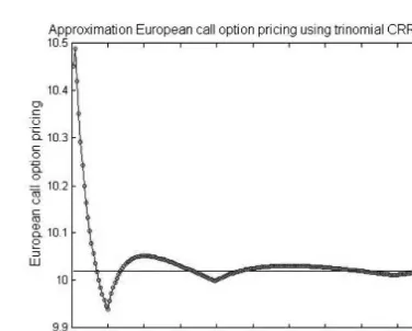
Figure 1. European call option pricing using CRR trinomial model with S0 = 100, K = 110, T = 1,
r = 0.05, s = 0.3, for n = 1, . . ., 200
Type of Option European Option Pricing Black-Scholes
n = 50 n = 100 n = 175 n = 200
European Call 10.0451 10.0257 10.0125 10.0205 10.0201
European Put 14.6804 14.6609 14.6478 14.6557 14.6553
Table 2. Call and put European Option Pricing use CRR Trinomial models
Type of Option European Option Pricing Black-Scholes
n = 50 n = 100 n = 175 n = 242
European Call 10.0274 10.0195 10.0263 10.0202 10.0201
European Put 14.6626 14.6547 14.6615 14.6554 14.6553
Table 3. Call and put European Option Pricing use Boyle Trinomial models
Type of Option European Option Pricing Black-Scholes
n = 100 n = 200 n = 350 n = 400
European Call 10.0451 10.0257 10.0125 10.0205 10.0201
European Put 14.6804 14.6609 14.6478 14.6557 14.6553
Figure 2. European call option pricing using Boyle trinomial model with S0 = 100, K = 110, T = 1,
r = 0.05, s = 0.3, for n = 1, . . ., 200
Figure 3. European put option pricing using CRR trinomial model with S0 = 100, K = 110, T = 1,
r = 0.05, s = 0.3, for n = 1, . . ., 200
Figure 4. European put option pricing using Boyle trinomial model with S0 = 100, K = 110, T = 1,
r = 0.05, s = 0.3, for n = 1, . . ., 200
Based on figure 1 – figure 4 can be known that although European option pricing CRR trinomial models and Boyle trinomial models is an approximation of European option pricing Black-Scholes when n increasingly larger, but it turns out that convergence of European option pricing trinomial models is not monotonous, but still better than binomial models, it can be seen clearly from European option pricing trinomial models charts that moves up and down but not too volatile.
The unarragement movement of European option pricing trinomial models, resulting the option price convergence is not monotonous, but the order convergence of European option pricing trinomial models can be determined. Basically European option pricing which obtained by using trinomial models will not be the same as European Black-Scholes option pricing. Therefore, there is a difference between European option pricing trinomial models with European Black-Scholes option pricing. The difference between option pricing is referred as error. Error value of both the option price is defined as follows:
en=
[
c (t0, S0) – cn(t0, S0)]
(17)
By applying the central limit theorem in equation (18) is obtained that
lim en 0 (18)
n
This means that option pricing is determined using trinomial models will converge towards option pricing is determined using Black-Scholes formula.
Basically, it is possible to determine in what order the option pricing convergence is obtained. This may be done to determine the exact upper boundary for the equation (20). Therefore, to explain order of convergence as required under this definition (Leisen & Reimer, 1996).
Definisi 5 (Leisen & Reimer, 1996)
option. A sequence of lattices converges with order r > 0 if there exists a constant k > 0 such that
en≤ k
nr'
∀n N
(19)
Furthermore, by applying the logarithm to the equation (19), be obtained
log (en) ≤log k – r log n
where it is shown that the logarithm error as a
function of log n will be located below a straight
line with a slope (slope) – r.
A lattice approach converges with order r > 0 if for all S0, K, r, s, T the specified sequence of lattices
converges with order r > 0 and denote this with
en = O( n1r )
. Please note that convergence of option valuation is implied by any order greater than 0. Higher order means more quickly convergence. Thus the theoretical concept of order of convergence is not unique: a lattice
approach with order r has also order . Order
of convergence is very easy to observe in actual simulations: in figures we plot the error against the refinement n on a log-log-scale (Leisen & Reimer, 1996). The following will be presented simulation error of European option pricing trinomial models with S0 = 100, K = 110, T = 1, r = 0.05, s = 0.3, for n = 1, . . ., 200.
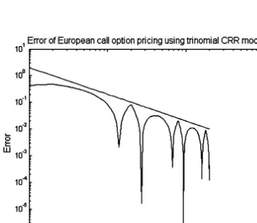
Figure 5. Error of the European call option pricing CRR trinomial models
with S0 = 100, K = 110, T = 1, r = 0.05, s = 0.3, for n = 1, . . ., 242 using log-log scale
with kappa = 3.5, lambda = 1.5
Figure 6. Error of the European put option pricing CRR trinomial models with S0 = 100, K = 110, T = 1, r = 0.05, s = 0.3, for n = 1, . . ., 242 using log-log
scale with kappa = 3.5, lambda = 1.5
Based on the simulation in the direction of European option pricing CRR trinomial models
above obtained kappa value is 2 and r = 1.5.
Therefore order of convergence for European option pricing trinomial CRR models in this simulation is 1.5. The following will be presented simulation error of European option pricing Boyle
trinomial models with S0 = 100, K = 110, T = 1, r
= 0.05, s = 0.3, for n = 1, . . ., 242.
Figure 7. Error of the European call option pricing Boyle trinomial models with S0 = 100, K = 110, T =
1, r = 0.05, s = 0.3, for n = 1, . . ., 242 using log-log
Figure 8. Error of the European put option pricing Boyle trinomial models with S0 = 100, K = 110, T =
1, r = 0.05, s = 0.3, for n = 1, . . ., 242 using log-log
scale with kappa = 3.5, lambda = 1.78
Based on the simulation in the direction of European option pricing Boyle trinomial models above obtained kappa value is 3.5 with lamda =
1.78 and r = 1.85. Therefore order of convergence
for European option pricing Boyle trinomial models in this simuation is 1.85.
CONCLUSION
Based on the overall analysis and simulations that have been done previously it can be concluded as follows:
1. European option pricing trinomial models for increasingly larger n will converge to Black-Scholes option pricing. Convergence of European option pricing trinomial models still not monotonous but rather steady than binomial models. European option pricing trinomial models more quickly converge to Black-Scholes option pricing than European option pricing binomial models.
2. According numerically analysis by simulation known that order of convergence for trinomial models constructed from CRR binomial models is one point five, whereas order of convergence for trinomial models proposed by Boyle to construct of the basic assumptions and restrictions general binomial models is one point eight five. Generally, order of convergence trinomial models has value more than one.
R E F E R E N C E S
Boyle, P. (1986). Option Valuation Using a Three-Jump Process. International Options Journal, Vol. 3, 7-12.
Boyle, P. (1988). A Lattice Framework for Option Pricing with Two State Variables. Journal of Financial and Quantitative Analysis, Vol 3, pp. 1-12.
Cox, J., Ross, S.A., Rubinstein M. (1979), Option Pricing: A Simplified Approach, Journal of Financial Economics 7, 229-263 Jarrow, R. & Rudd, A. (1982) Approximate option valuation for arbitrary stochastic processes. Journal of Financial Economics,
Vol. 10, pp. 347-369.
John Hull and Alan White, «Pricing interest-rate derivative securities», The Review of Financial Studies, Vol 3, No. 4 (1990) pp. 573–592
Leisen, Dietmar., Matthias Reimer. (1996), Binomial models for option valuation-examining and improving convergence, Applied Mathematical Finance, 3, 319-346.
Takahashi, H. (2000), A Note on Pricing Derivatives in an Incomplete Markets, Hitotsubashi University.
Tian, Y. (1999). A flexible binomial option pricing model. The Journal of Futures Markets, Vol. 19, No. 7, pp. 817-843.