A M I T S A H A
D O I N G M A T H
W I T H P Y T H O N
D O I N G M A T H
W I T H P Y T H O N
U S E P R O G R A M M I N G T O E X P L O R E
A L G E B R A
,S T A T I S T I C S
,C A L C U L U S
, A N D M O R E !•
•
•
•
D O I N G M A T H
W I T H P Y T H O N
U s e P r o g r a m m i n g t o
E x p l o r e A l g e b r a , S t a t i s t i c s ,
C a l c u l u s , a n d M o r e !
by Amit Saha
DOING MATH WITH PYTHON. Copyright © 2015 by Amit Saha.
All rights reserved. No part of this work may be reproduced or transmitted in any form or by any means, electronic or mechanical, including photocopying, recording, or by any information storage or retrieval system, without the prior written permission of the copyright owner and the publisher.
Printed in USA
Developmental Editors: Seph Kramer and Tyler Ortman Technical Reviewer: Jeremy Kun
Copyeditor: Julianne Jigour Compositor: Riley Hoffman Proofreader: Paula L. Fleming
For information on distribution, translations, or bulk sales, please contact No Starch Press, Inc. directly:
No Starch Press, Inc.
245 8th Street, San Francisco, CA 94103 phone: 415.863.9900; [email protected] www.nostarch.com
Library of Congress Cataloging-in-Publication Data Saha, Amit, author.
Doing math with Python : use programming to explore algebra, statistics, calculus, and more! / by Amit Saha.
pages cm
Summary: "Uses the Python programming language as a tool to explore high school-level mathematics like statistics, geometry, probability, and calculus by writing programs to find derivatives, solve equations graphically, manipulate algebraic expressions, and examine projectile motion. Covers programming concepts including using functions, handling user input, and reading and manipulating data"-- Provided by publisher.
Includes index.
ISBN 978-1-59327-640-9 -- ISBN 1-59327-640-0
1. Mathematics--Study and teaching--Data processing. 2. Python (Computer program language) 3. Computer programming. I. Title.
QA20.C65S24 2015 510.285'5133--dc23
2015009186
No Starch Press and the No Starch Press logo are registered trademarks of No Starch Press, Inc. Other product and company names mentioned herein may be the trademarks of their respective owners. Rather than use a trademark symbol with every occurrence of a trademarked name, we are using the names only in an editorial fashion and to the benefit of the trademark owner, with no intention of infringement of the trademark.
B R I E F C O N T E N T S
Acknowledgments . . . xiii
Introduction . . . xv
Chapter 1: Working with Numbers . . . 1
Chapter 2: Visualizing Data with Graphs . . . 27
Chapter 3: Describing Data with Statistics. . . 61
Chapter 4: Algebra and Symbolic Math with SymPy . . . 93
Chapter 5: Playing with Sets and Probability . . . 121
Chapter 6: Drawing Geometric Shapes and Fractals . . . 149
Chapter 7: Solving Calculus Problems . . . 177
Afterword . . . 209
Appendix A: Software Installation . . . 213
Appendix B: Overview of Python Topics . . . 221
#3: Enhanced Projectile Trajectory Comparison Program . . . 56
#4: Visualizing Your Expenses . . . 56
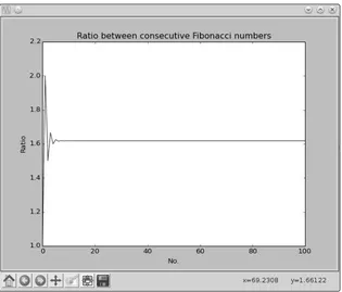
#5: Exploring the Relationship Between the Fibonacci Sequence and the Golden Ratio . . . 59
5
PLAYING WITH SETS AND PROBABILITY 121
A C K N O W L E D G M E N T S
I would like to thank everyone at No Starch Press for making this book possible. From the first emails discussing the book idea with Bill Pollock and Tyler Ortman, through the rest of the process, everyone there has been an absolute pleasure to work with. Seph Kramer was amazing with his technical insights and suggestions and Riley Hoffman was meticulous in checking and re-checking that everything was correct. It is only fair to say that without these two fine people, this book wouldn’t have been close to what it is. Thanks to Jeremy Kun and Otis Chodosh for their insights and making sure all the math made sense. I would also like to thank the copy-editor, Julianne Jigour, for her thoroughness.
SymPy forms a core part of many chapters in this book and I would like to thank everyone on the SymPy mailing list for answering my queries patiently and reviewing my patches with promptness. I would also like to thank the matplotlib community for answering and clearing up my doubts.
I would like to thank David Ash for lending me his Macbook, which helped me when writing the software installation instructions.
I N T R O D U C T I O N
This book’s goal is to bring together three
topics near to my heart—programming,
math, and science. What does that mean
exactly? Within these pages, we’ll
programmati-cally explore high school–level topics, like manipulating
units of measurement; examining projectile motion;
calculating mean, median, and mode; determining linear correlation; solving algebraic equations; describing the motion of a simple pendulum; simulating dice games; creating geometric shapes; and finding the limits, derivatives, and integrals of functions. These are familiar topics for many, but instead of using pen and paper, we’ll use our computer to explore them.
among other tasks. In other programs, we’ll simulate real-life events, such as projectile motion, a coin toss, or a die roll. Using programs to simulate such events gives us an easy way to analyze and learn more about them.
You’ll also find topics that would be extremely difficult to explore with-out programs. For example, drawing fractals by hand is tedious at best and close to impossible at worst. With a program, all we need to do is run a for
loop with the relevant operation in the body of the loop.
I think you’ll find that this new context for “doing math” makes learn-ing both programmlearn-ing and math more excitlearn-ing, fun, and rewardlearn-ing.
Who Should Read This Book
If you yourself are learning programming, you’ll appreciate how this book demonstrates ways to solve problems with computers. Likewise, if you teach such learners, I hope you find this book useful to demonstrate the applica-tion of programming skills beyond the sometimes abstract world of com-puter science.
This book assumes the reader knows the absolute basics of Python programming using Python 3—specifically, what a function is, function arguments, the concept of a Python class and class objects, and loops. Appendix B covers some of the other Python topics that are used by the programs, but this book doesn’t assume knowledge of these additional topics. If you find yourself needing more background, I recommend reading Python for Kids by Jason Briggs (No Starch Press, 2013).
What’s in This Book?
This book consists of seven chapters and two appendices. Each chapter ends with challenges for the reader. I recommend giving these a try, as there’s much to learn from trying to write your own original programs. Some of these challenges will ask you to explore new topics, which is a great way to enhance your learning.
• Chapter 1, Working with Numbers, starts off with basic mathematical operations and gradually moves on to topics requiring a higher level of math know-how.
• Chapter 2, Visualizing Data with Graphs, discusses creating graphs from data sets using the matplotlib library.
• Chapter 4, Algebra and Symbolic Math with SymPy, introduces sym-bolic math using the SymPy library. It begins with the basics of repre-senting and manipulating algebraic expressions before introducing more complicated matters, such as solving equations.
• Chapter 5, Playing with Sets and Probability, discusses the representa-tion of mathematical sets and moves on to basic discrete probability. You’ll also learn to simulate uniform and nonuniform random events. • Chapter 6, Drawing Geometric Shapes and Fractals, discusses using
matplotlib to draw geometric shapes and fractals and create animated figures.
• Chapter 7, Solving Calculus Problems, discusses some of the math-ematical functions available in the Python standard library and SymPy and then introduces you to solving calculus problems.
• Appendix A, Software Installation, covers installation of Python 3, matplotlib, and SymPy on Microsoft Windows, Linux, and Mac OS X. • Appendix B, Overview of Python Topics, discusses several Python
topics that may be helpful for beginners.
Scripts, Solutions, and Hints
This book’s companion site is http://www.nostarch.com/doingmathwithpython/. Here, you can download all the programs in this book as well as hints and solutions for the challenges. You’ll also find links to additional math, science, and Python resources I find useful as well as any corrections or updates to the book itself.
1
W O R K I N G W I T H N U M B E R S
Let’s take our first steps toward using
Python to explore the world of math and
science. We’ll keep it simple now so you can
get a handle on using Python itself. We’ll start
by performing basic mathematical operations, and
then we’ll write simple programs for manipulating
and understanding numbers. Let’s get started!
Basic Mathematical Operations
Figure 1-1: Python 3 IDLE shell
Python can act like a glorified calculator, doing simple computations. Just type an expression and Python will evaluate it. After you press ENTER,
the result appears immediately.
Give it a try. You can add and subtract numbers using the addition (+) and subtraction (–) operators. For example:
>>> 1 + 2
3
>>> 1 + 3.5
4.5
>>> -1 + 2.5
1.5
>>> 100 – 45
55
>>> -1.1 + 5
3.9
To multiply, use the multiplication (*) operator:
>>> 3 * 2
6
>>> 3.5 * 1.5
5.25
To divide, use the division (/) operator:
>>> 3 / 2
1.5 >>> 4 / 2
2.0
As you can see, when you ask Python to perform a division operation, it returns the fractional part of the number as well. If you want the result in the form of an integer, with any decimal values removed, you should use the floor division (//) operator:
>>> 3 // 2
The floor division operator divides the first number by the second number and then rounds down the result to the next lowest integer. This becomes interesting when one of the numbers is negative. For example:
>>> -3 // 2
-2
The final result is the integer lower than the result of the division oper-ation (-3/2 = -1.5, so the final result is -2).
On the other hand, if you want just the remainder, you should use the modulo (%) operator:
>>> 9 % 2
1
You can calculate the power of numbers using the exponential (**) operator. The examples below illustrate this:
>>> 2 ** 2
4
>>> 2 ** 10
1024 >>> 1 ** 10
1
We can also use the exponential symbol to calculate powers less than 1. For example, the square root of a number n can be expressed as n1/2 and the cube root as n1/3:
>>> 8 ** (1/3)
2.0
As this example shows, you can use parentheses to combine mathe-matical operations into more complicated expressions. Python will evalu-ate the expression following the standard PEMDAS rule for the order of calculations—parentheses, exponents, multiplication, division, addition, and subtraction. Consider the following two expressions—one without parentheses and one with:
>>> 5 + 5 * 5
30
>>> (5 + 5) * 5
50
Labels: Attaching Names to Numbers
As we start designing more complex Python programs, we’ll assign names to numbers—at times for convenience, but mostly out of necessity. Here’s a simple example: evaluate the result of the expression a + 1, it sees that the number that
a refers to is 3, and then it adds 1 and displays the output (4). At v, we change the value of a to 5, and this is reflected in the second addition operation. Using the name a is convenient because you can simply change the number that a points to and Python uses this new value when a is referred to anywhere after that.
This kind of name is called a label. You may have been introduced to the term variable to describe the same idea elsewhere. However, consider-ing that variable is also a mathematical term (used to refer to somethconsider-ing like x in the equation x + 2 = 3), in this book I use the term variable only in the context of mathematical equations and expressions.
Different Kinds of Numbers
You may have noticed that I’ve used two kinds of numbers to demonstrate the mathematical operations—numbers without a decimal point, which you already know as integers, and numbers with a decimal point, which program-mers call floating point numbers. We humans have no trouble recognizing and working with numbers whether they’re written as integers, floating point decimals, fractions, or roman numerals. But in some of the programs that we write in this book, it will only make sense to perform a task on a particular type of number, so we’ll often have to write a bit of code to have the programs check whether the numbers we input are of the right type.
Python considers integers and floating point numbers to be different types. If you use the function type(), Python will tell you what kind of num-ber you’ve just input. For example:
Here, you can see that Python classifies the number 3 as an integer (type 'int') but classifies 3.0 as a floating point number (type 'float'). We all know that 3 and 3.0 are mathematically equivalent, but in many situa-tions, Python will treat these two numbers differently because they are two different types.
Some of the programs we write in this chapter will work properly only with an integer as an input. As we just saw, Python won’t recognize a num-ber like 1.0 or 4.0 as an integer, so if we want to accept numnum-bers like that as valid input in these programs, we’ll have to convert them from floating point numbers to integers. Luckily, there’s a function built in to Python that does just that:
>>> int(3.8)
3
>>> int(3.0)
3
The function int() takes the input floating point number, gets rid of anything that comes after the decimal point, and returns the resulting inte-ger. The float() function works similarly to perform the reverse conversion:
>>> float(3)
3.0
float() takes the integer that was input and adds a decimal point to turn it into a floating point number.
Working with Fractions
Python can also handle fractions, but to do that, we’ll need to use Python’s
fractions module. You can think of a module as a program written by someone else that you can use in your own programs. A module can include classes, functions, and even label definitions. It can be part of Python’s standard library or distributed from a third-party location. In the latter case, you would have to install the module before you could use it.
The fractions module is part of the standard library, meaning that it’s already installed. It defines a class Fraction, which is what we’ll use to enter fractions into our programs. Before we can use it, we’ll need to import it, which is a way of telling Python that we want to use the class from this mod-ule. Let’s see a quick example—we’ll create a new label, f, which refers to the fraction 3/4:
u >>> from fractions import Fraction
v >>> f = Fraction(3, 4)
w >>> f
denominator as parameters v. This creates a Fraction object for the frac-tion 3/4. When we print the object w, Python displays the fraction in the form Fraction(numerator, denominator).
The basic mathematical operations, including the comparison opera-tions, are all valid for fractions. You can also combine a fraction, an integer, and a floating point number in a single expression:
>>> Fraction(3, 4) + 1 + 1.5
3.25
When you have a floating point number in an expression, the result of the expression is returned as a floating point number.
On the other hand, when you have only a fraction and an integer in the expression, the result is a fraction, even if the result has a denominator of 1.
>>> Fraction(3, 4) + 1 + Fraction(1/4)
Fraction(2, 1)
Now you know the basics of working with fractions in Python. Let’s move on to a different kind of number.
Complex Numbers
The numbers we’ve seen so far are the so-called real numbers. Python also supports complex numbers with the imaginary part identified by the letter j or J (as opposed to the letter i used in mathematical notation). For example, the complex number 2 + 3i would be written in Python as 2 + 3j:
>>> a = 2 + 3j
>>> type(a)
<class 'complex'>
As you can see, when we use the type() function on a complex number, Python tells us that this is an object of type complex.
You can also define complex numbers using the complex() function:
>>> a = complex(2, 3)
>>> a
(2 + 3j)
Here we pass the real and imaginary parts of the complex number as two arguments to the complex() function, and it returns a complex number.
You can add and subtract complex numbers in the same way as real numbers:
>>> b = 3 + 3j
>>> a + b
(5 + 6j) >>> a - b
Multiplication and division of complex numbers are also carried out similarly:
>>> a * b
(-3 + 15j) >>> a / b
(0.8333333333333334 + 0.16666666666666666j)
The modulus (%) and the floor division (//) operations are not valid for complex numbers.
The real and imaginary parts of a complex number can be retrieved using its real and imag attributes, as follows:
>>> z = 2 + 3j
>>> z.real
2.0 >>> z.imag
3.0
The conjugate of a complex number has the same real part but an imagi-nary part with an equal magnitude and an opposite sign. It can be obtained using the conjugate() method:
>>> z.conjugate()
(2 - 3j)
Both the real and imaginary parts are floating point numbers. Using the real and imaginary parts, you can then calculate the magnitude of a complex number with the following formula, where x and y are the real and imaginary parts of the number, respectively: . In Python, this would look like the following:
>>> (z.real ** 2 + z.imag ** 2) ** 0.5
3.605551275463989
A simpler way to find the magnitude of a complex number is with the
abs() function. The abs() function returns the absolute value when called with a real number as its argument. For example, abs(5) and abs(-5) both return 5. However, for complex numbers, it returns the magnitude:
>>> abs(z)
3.605551275463989
Getting User Input
As we start to write programs, it will help to have a nice, simple way to accept user input via the input() function. That way, we can write programs that ask a user to input a number, perform specific operations on that num-ber, and then display the results of the operations. Let’s see it in action:
u >>> a = input()
v 1
At u, we call the input() function, which waits for you to type something, as shown at v, and press ENTER. The input provided is stored in a:
>>> a
w '1'
Notice the single quotes around 1 at w. The input() function returns the input as a string. In Python, a string is any set of characters between two quotes. When you want to create a string, either single quotes or double quotes can be used:
>>> s1 = 'a string'
>>> s2 = "a string"
Here, both s1 and s2 refer to the same string.
Even if the only characters in a string are numbers, Python won’t treat that string as a number unless we get rid of those quotation marks. So before we can perform any mathematical operations with the input, we’ll have to convert it into the correct number type. A string can be converted to an integer or floating point number using the int() or float() function, respectively:
>>> a = '1'
>>> int(a) + 1
2
>>> float(a) + 1
2.0
These are the same int() and float() functions we saw earlier, but this time instead of converting the input from one kind of number to another, they take a string as input ('1') and return a number (2 or 2.0). It’s impor-tant to note, however, that the int() function cannot convert a string con-taining a floating point decimal into an integer. If you take a string that has a floating point number (like '2.5' or even '2.0') and input that string into the int() function, you’ll get an error message:
>>> int('2.0')
File "<pyshell#26>", line 1, in <module> int('2.0')
ValueError: invalid literal for int() with base 10: '2.0'
This is an example of an exception—Python’s way of telling you that it cannot continue executing your program because of an error. In this case, the exception is of the type ValueError. (For a quick refresher on exceptions, see Appendix B.)
Similarly, when you supply a fractional number such as 3/4 as an input, Python cannot convert it into an equivalent floating point number or inte-ger. Once again, a ValueError exception is raised:
>>> a = float(input())
3/4
Traceback (most recent call last):
File "<pyshell#25>", line 1, in <module> a=float(input())
ValueError: could not convert string to float: '3/4'
You may find it useful to perform the conversion in a try...except block so that you can handle this exception and alert the user that the program has encountered an invalid input. We’ll look at try...except blocks next.
Handling Exceptions and Invalid Input
If you’re not familiar with try...except, the basic idea is this: if you execute one or more statements in a try...except block and there’s an error while executing, your program will not crash and print a Traceback. Instead, the execution is transferred to the except block, where you can perform an appropriate operation, for instance, printing a helpful error message or trying something else.
This is how you would perform the above conversion in a try...except
block and print a helpful error message on invalid input:
>>> try:
a = float(input('Enter a number: ')) except ValueError:
print('You entered an invalid number')
Note that we need to specify the type of exception we want to handle. Here, we want to handle the ValueError exception, so we specify it as except ValueError.
Now, when you give an invalid input, such as 3/4, it prints a helpful error message, as shown at u:
Enter a number: 3/4
You can also specify a prompt with the input() function to tell the user what kind of input is expected. For example:
>>> a = input('Input an integer: ')
The user will now see the message hinting to enter an integer as input:
Input an integer: 1
In many programs in this book, we’ll ask the user to enter a number as input, so we’ll have to make sure we take care of conversion before we attempt to perform any operations on these numbers. You can combine the input and conversion in a single statement, as follows:
>>> a = int(input())
1
>>> a + 1
2
This works great if the user inputs an integer. But as we saw earlier, if the input is a floating point number (even one that’s equivalent to an inte-ger, like 1.0), this will produce an error:
>>> a = int(input()) 1.0
Traceback (most recent call last):
File "<pyshell#42>", line 1, in <module> a=int(input())
ValueError: invalid literal for int() with base 10: '1.0'
In order to avoid this error, we could set up a ValueError catch like the one we saw earlier for fractions. That way the program would catch float-ing point numbers, which won’t work in a program meant for integers. However, it would also flag numbers like 1.0 and 2.0, which Python sees as floating point numbers but that are equivalent to integers and would work just fine if they were entered as the right Python type.
To get around all this, we will use the is_integer() method to filter out any numbers with a significant digit after the decimal point. (This method is only defined for float type numbers in Python; it won’t work with num-bers that are already entered in integer form.)
Here’s an example:
>>> 1.1.is_integer()
False
hand, when the method is called with 1.0 as the floating point number, the result is True:
>>> 1.0.is_integer()
True
We can use is_integer() to filter out noninteger input while keeping inputs like 1.0, which is expressed as a floating point number but is equiva-lent to an integer. We’ll see how the method would fit into a larger program a bit later.
Fractions and Complex Numbers as Input
The Fraction class we learned about earlier is also capable of converting a string such as '3/4' to a Fraction object. In fact, this is how we can accept a fraction as an input:
>>> a = Fraction(input('Enter a fraction: '))
Enter a fraction: 3/4
>>> a
Fraction(3, 4)
Try entering a fraction such as 3/0 as input:
>>> a = Fraction(input('Enter a fraction: '))
Enter a fraction: 3/0
Traceback (most recent call last): File "<pyshell#2>", line 1, in <module> a = Fraction(input('Enter a fraction: '))
File "/usr/lib64/python3.3/fractions.py", line 167, in __new__ raise ZeroDivisionError('Fraction(%s, 0)' % numerator) ZeroDivisionError: Fraction(3, 0)
The ZeroDivisionError exception message tells you (as you already know) that a fraction with a denominator of 0 is invalid. If you’re planning on hav-ing users enter fractions as input in one of your programs, it’s a good idea to always catch such exceptions. Here is how you can do something like that:
>>> try:
a = Fraction(input('Enter a fraction: ')) except ZeroDivisionError:
print('Invalid fraction')
Enter a fraction: 3/0
Invalid fraction
Similarly, the complex() function can convert a string such as '2+3j' into a complex number:
>>> z = complex(input('Enter a complex number: '))
Enter a complex number: 2+3j
>>> z
(2+3j)
If you enter the string as '2 + 3j' (with spaces), it will result in a
ValueError error message:
>>> z = complex(input('Enter a complex number: '))
Enter a complex number: 2 + 3j
Traceback (most recent call last):
File "<pyshell#43>", line 1, in <module>
z = complex(input('Enter a complex number: ')) ValueError: complex() arg is a malformed string
It’s a good idea to catch the ValueError exception when converting a string to a complex number, as we’ve done for other number types.
Writing Programs That Do the Math for You
Now that we have learned some of the basic concepts, we can combine them with Python’s conditional and looping statements to make some programs that are a little more advanced and useful.
Calculating the Factors of an Integer
When a nonzero integer, a, divides another integer, b, leaving a remainder 0, a is said to be a factor of b. As an example, 2 is a factor of all even integers. We can write a function such as the one below to find whether a nonzero integer, a, is a factor of another integer, b:
>>> def is_factor(a, b): if b % a == 0: return True else:
return False
We use the % operator introduced earlier in this chapter to calculate the remainder. If you ever find yourself asking a question like “Is 4 a factor of 1024?”, you can use the is_factor() function:
>>> is_factor(4, 1024)
True
range() function to write a program that will go through each of those num-bers between 1 and n.
Before we write the full program, let’s take a look at how range() works. A typical use of the range() function looks like this:
>>> for i in range(1, 4): print(i)
1 2 3
Here, we set up a for loop and gave the range function two arguments. The range() function starts from the integer stated as the first argument (the start value) and continues up to the integer just before the one stated by the second argument (the stop value). In this case, we told Python to print out the numbers in that range, beginning with 1 and stopping at 4. Note that this means Python doesn’t print 4, so the last number it prints is the number before the stop value (3). It’s also important to note that the
range() function accepts only integers as its arguments.
You can also use the range() function without specifying the start value, in which case it’s assumed to be 0. For example:
>>> for i in range(5): print(i)
The difference between two consecutive integers produced by the
range() function is known as the step value. By default, the step value is 1. To specify a different step value, specify it as the third argument (the start value is not optional when you specify a step value). For example, the follow-ing program prints the odd numbers below 10:
>>> for i in range(1,10,2): print(i)
three straight single quotes ('). The text in between those quotes won’t be executed by Python as part of the program; it’s just commentary for us humans.
'''
Find the factors of an integer '''
The factors() function defines a for loop that iterates once for every integer between 1 and the input integer at u using the range() function. Here, we want to iterate up to the integer entered by the user, b, so the stop value is stated as b+1. For each of these integers, i, the program checks whether it divides the input number with no remainder and prints it if so.
When you run this program (by selecting Run4Run Module), it asks you to input a number. If your number is a positive integer, its factors are printed. For example:
Your Number Please: 25
1 5 25
If you enter a non-integer or a negative integer as an input, the pro-gram prints an error message asking you to input a positive integer:
Your Number Please: 15.5
Please enter a positive integer
This is an example of how we can make programs more user friendly by always checking for invalid input in the program itself. Because our program works only for finding the factors of a positive integer, we check whether the input number is greater than 0 and is an integer using the
Generating Multiplication Tables
Consider three numbers, a, b, and n, where n is an integer, such that
a × n = b.
We can say here that b is the nth multiple of a. For example, 4 is the 2nd multiple of 2, and 1024 is the 512nd multiple of 2.
A multiplication table for a number lists all of that number’s multiples. For example, the multiplication table of 2 looks like this (first three mul-tiples shown here):
2 × 1 = 2
2 × 2 = 4
2 × 3 = 6
Our next program generates the multiplication number up to 10 for any number input by the user. In this program, we’ll use the format()
method with the print() function to help make the program’s output look nicer and more readable. In case you haven’t seen it before, I’ll now briefly explain how it works.
The format() method lets you plug in labels and set it up so that they get printed out in a nice, readable string with extra formatting around it. For example, if I had the names of all the fruits I bought at the grocery store with separate labels created for each and wanted to print them out to make a coherent sentence, I could use the format() method as follows:
>>> item1 = 'apples'
>>> item2 = 'bananas'
>>> item3 = 'grapes'
>>> print('At the grocery store, I bought some {0} and {1} and {2}'.format(item1, item2, item3))
At the grocery store, I bought some apples and bananas and grapes
First, we created three labels (item1, item2, and item3), each referring to a different string (apples, bananas, and grapes). Then, in the print() function, we typed a string with three placeholders in curly brackets: {0}, {1}, and {2}. We followed this with .format(), which holds the three labels we created. This tells Python to fill those three placeholders with the values stored in those labels in the order listed, so Python prints the text with {0} replaced by the first label, {1} replaced by the second label, and so on.
It’s not necessary to have labels pointing to the values we want to print. We can also just type values into .format(), as in the following example:
>>> print('Number 1: {0} Number 2: {1} '.format(1, 3.578))
Number 1: 1 Number 2: 3.578
Now that we’ve seen how format() works, we’re ready to take a look at the program for our multiplication table printer:
'''
The function multi_table() implements the main functionality of the program. It takes the number for which the multiplication table will be printed as a parameter, a. Because we want to print the multiplication table from 1 to 10, we have a for loop at u that iterates over each of these num-bers, printing the product of itself and the number, a.
When you execute the program, it asks you to input a number, and the program prints its multiplication table:
See how nice and orderly that table looks? That’s because we used the
.format() method to print the output according to a readable, uniform template.
You can use the format() method to further control how numbers are printed. For example, if you want numbers with only two decimal places, you can specify that with the format() method. Here is an example:
>>> '{0}'.format(1.25456)
'1.25456'
>>> '{0:.2f}'.format(1.25456)
'1.25'
meaning that we want only two numbers after the decimal point, with the f
indicating a floating point number. As you can see, there are only two num-bers after the decimal point in the next output. Note that the number is rounded if there are more numbers after the decimal point than you speci-fied. For example:
>>> '{0:.2f}'.format(1.25556)
'1.26'
Here, 1.25556 is rounded up to the nearest hundredth and printed as 1.26. If you use .2f and the number you are printing is an integer, zeros are added at the end:
>>> '{0:.2f}'.format(1)
'1.00'
Two zeros are added because we specified that we should print exactly two numbers after the decimal point.
Converting Units of Measurement
The International System of Units defines seven base quantities. These are then used to derive other quantities, referred to as derived quantities. Length (including width, height, and depth), time, mass, and temperature are four of the seven base quantities. Each of these quantities has a standard unit of measurement: meter, second, kilogram, and kelvin, respectively.
But each of these standard measurement units also has multiple non-standard measurement units. You are more familiar with the temperature being reported as 30 degrees Celsius or 86 degrees Fahrenheit than as 303.15 kelvin. Does that mean 303.15 kelvin feels three times hotter than 86 degrees Fahrenheit? No way! We can’t compare 86 degrees Fahrenheit to 303.15 kelvin only by their numerical values because they’re expressed in different measurement units, even though they measure the same physical quantity—temperature. You can compare two measurements of a physical quantity only when they’re expressed in the same unit of measurement.
Conversions between different units of measurement can be tricky, and that’s why you’re often asked to solve problems that involve conversion between different units of measurement in high school. It’s a good way to test your basic mathematical skills. But Python has plenty of math skills, too, and, unlike some high school students, it doesn’t get tired of crunch-ing numbers over and over again in a loop! Next, we’ll explore writcrunch-ing pro-grams to perform those unit conversions for you.
divide the measurement in centimeters by 100 to obtain the measurement in meters. For example, here’s how you can convert 25.5 inches to meters:
>>> (25.5 * 2.54) / 100
0.6476999999999999
On the other hand, a mile is roughly equivalent to 1.609 kilometers. So if you see that your destination is 650 miles away, you’re 650 × 1.609 kilome-ters away:
>>> 650 * 1.609
1045.85
Now let’s take a look at temperature conversion—converting tempera-ture from Fahrenheit to Celsius and vice versa. Temperatempera-ture expressed in Fahrenheit is converted into its equivalent value in Celsius using the formula
.
F is the temperature in Fahrenheit, and C is its equivalent in Celsius. You know that 98.6 degrees Fahrenheit is said to be the normal human body temperature. To find the corresponding temperature in degrees Celsius, we evaluate the above formula in Python:
>>> F = 98.6
>>> (F - 32) * (5 / 9)
37.0
First, we create a label, F, with the temperature in Fahrenheit, 98.6. Next, we evaluate the formula for converting this temperature to its equiva-lent in Celsius, which turns out be 37.0 degrees Celsius.
To convert temperature from Celsius to Fahrenheit, you would use the formula
.
You can evaluate this formula in a similar manner:
>>> C = 37
>>> C * (9 / 5) + 32
98.60000000000001
We create a label, C, with the value 37 (the normal human body tem-perature in Celsius). Then, we convert it into Fahrenheit using the formula, and the result is 98.6 degrees.
for us. This program will present a menu to allow users to select the conver-sion they want to perform, ask for relevant input, and then print the calcu-lated result. The program is shown below:
'''
Unit converter: Miles and Kilometers '''
def print_menu():
print('1. Kilometers to Miles') print('2. Miles to Kilometers')
def km_miles():
km = float(input('Enter distance in kilometers: ')) miles = km / 1.609
print('Distance in miles: {0}'.format(miles))
def miles_km():
miles = float(input('Enter distance in miles: ')) km = miles * 1.609
print('Distance in kilometers: {0}'.format(km))
if __name__ == '__main__':
u print_menu()
v choice = input('Which conversion would you like to do?: ') if choice == '1':
km_miles()
if choice == '2': miles_km()
This is a slightly longer program than the others, but not to worry. It’s actually simple. Let’s start from u. The print_menu() function is called, which prints a menu with two unit conversion choices. At v, the user is asked to select one of the two conversions. If the choice is entered as 1 (kilometers to miles), the function km_miles() is called. If the choice is entered as 2 (miles to kilometers), the function miles_km() is called. In both of these functions, the user is first asked to enter a distance in the unit chosen for conversion (kilometers for km_miles() and miles for miles_km()). The program then performs the conversion using the corresponding for-mula and displays the result.
Here is a sample run of the program:
1. Kilometers to Miles 2. Miles to Kilometers
u Which conversion would you like to do?: 2
The user is asked to enter a choice at u. The choice is entered as 2 (miles to kilometers). The program then asks the user to enter the distance in miles to be converted to kilometers and prints the conversion.
This program just converts between miles and kilometers, but in a programming challenge later, you’ll extend this program so that it can perform conversions of other units.
Finding the Roots of a Quadratic Equation
What do you do when you have an equation such as x + 500 – 79 = 10 and you need to find the value of the unknown variable, x? You rearrange the terms such that you have only the constants (500, –79, and 10) on one side of the equation and the variable (x) on the other side. This results in the following equation: x = 10 – 500 + 79.
Finding the value of the expression on the right gives you the value of x, your solution, which is also called the root of this equation. In Python, you can do this as follows:
>>> x = 10 - 500 + 79
>>> x
-411
This is an example of a linear equation. Once you have rearranged the terms on both sides, the expression is simple enough to evaluate. On the other hand, for equations such as x2 + 2x + 1 = 0, finding the roots of x usu-ally involves evaluating a complex expression known as the quadratic formula. Such equations are known as quadratic equations, generally expressed as ax2 + bx + c = 0, where a, b, and c are constants. The quadratic formula for calculating the roots is given as follows:
and .
A quadratic equation has two roots—two values of x for which the two sides of the quadratic equation are equal (although sometimes these two values may turn out to be the same). This is indicated here by the x1 and x2 in the quadratic formula.
Comparing the equation x2 + 2x + 1 = 0 to the generic quadratic equation, we see that a = 1, b = 2, and c = 1. We can substitute these values directly into the quadratic formula to calculate the value of x1 and x2. In Python, we first store the values of a, b, and c as the labels a, b, and c with the appropriate values:
>>> a = 1
>>> b = 2
Then, considering that both the formulas have the term b2 – 4ac, we’ll define a new label with D, such that :
>>> D = (b**2 – 4*a*c)**0.5
As you can see, we evaluate the square root of b2 – 4ac by raising it to the 0.5th power. Now, we can write the expressions for evaluating x1 and x2:
>>> x_1 = (-b + D)/(2*a)
>>> x_1
-1.0
>>> x_2 = (-b - D)/(2*a)
>>> x_2
-1.0
In this case, the values of both the roots are the same, and if you substi-tute that value into the equation x2 + 2x + 1, the equation will evaluate to 0.
Our next program combines all these steps in a function roots(), which takes the values of a, b, and c as parameters, calculates the roots, and prints them:
'''
Quadratic equation root calculator '''
def roots(a, b, c):
D = (b*b - 4*a*c)**0.5 x_1 = (-b + D)/(2*a) x_2 = (-b - D)/(2*a)
print('x1: {0}'.format(x_1)) print('x2: {0}'.format(x_2))
if __name__ == '__main__': a = input('Enter a: ') b = input('Enter b: ') c = input('Enter c: ')
roots(float(a), float(b), float(c))
At first, we use the labels a, b, and c to reference the values of the three constants of a quadratic equation. Then, we call the roots() function with these three values as arguments (after converting them to floating point numbers). This function plugs a, b, and c into the quadratic formula, finds the roots for that equation, and prints them.
x1: -1.000000 x2: -1.000000
Try solving a few more quadratic equations with different values for the constants, and the program will find the roots correctly.
You most likely know that quadratic equations can have complex num-bers as roots, too. For example, the roots of the equation x2 + x + 1 = 0 are both complex numbers. The above program can find those for you as well. Let’s give it a shot by executing the program again (the constants are a = 1, b = 1, and c = 1):
Enter a: 1
Enter b: 1
Enter c: 1
x1: (-0.49999999999999994+0.8660254037844386j) x2: (-0.5-0.8660254037844386j)
The roots printed above are complex numbers (indicated by j), and the program has no problem calculating or displaying them.
What You Learned
Great work on finishing the first chapter! You learned to write programs that recognize integers, floating point numbers, fractional numbers (expressed as a fraction or a floating point number), and complex numbers. You wrote programs that generate multiplication tables, perform unit conversions, and find the roots of a quadratic equation. I’m sure you’re already excited about having taken the first steps toward writing programs that will do mathemati-cal mathemati-calculations for you. Before we move on, here are some programming challenges that will give you a chance to further apply what you’ve learned.
Programming Challenges
Here are a few challenges that will give you a chance to practice the concepts from this chapter. Each problem can be solved in multiple ways, but you can find sample solutions at http://www.nostarch.com/doingmathwithpython/.
#1: Even-Odd Vending Machine
Try writing an “even-odd vending machine,” which will take a number as input and do two things:
1. Print whether the number is even or odd.
2. Display the number followed by the next 9 even or odd numbers.
Your program should use the is_integer() method to display an error message if the input is a number with significant digits beyond the decimal point.
#2: Enhanced Multiplication Table Generator
Our multiplication table generator is cool, but it prints only the first 10 mul-tiples. Enhance the generator so that the user can specify both the number and up to which multiple. For example, I should be able to input that I want to see a table listing the first 15 multiples of 9.
#3: Enhanced Unit Converter
The unit conversion program we wrote in this chapter is limited to conver-sions between kilometers and miles. Try extending the program to convert between units of mass (such as kilograms and pounds) and between units of temperature (such as Celsius and Fahrenheit).
#4: Fraction Calculator
Write a calculator that can perform the basic mathematical operations on two fractions. It should ask the user for two fractions and the operation the user wants to carry out. As a head start, here’s how you can write the pro-gram with only the addition operation:
'''
Fraction operations '''
from fractions import Fraction
def add(a, b):
print('Result of Addition: {0}'.format(a+b))
if __name__ == '__main__':
u a = Fraction(input('Enter first fraction: '))
v b = Fraction(input('Enter second fraction: '))
op = input('Operation to perform - Add, Subtract, Divide, Multiply: ') if op == 'Add':
add(a,b)
You’ve already seen most of the elements in this program. At u and v, we ask the user to input the two fractions. Then, we ask the user which operation is to be performed on the two fractions. If the user enters 'Add'
as input, we call the function add(), which we’ve defined to find the sum of the two fractions passed as arguments. The add() function performs the operation and prints the result. For example:
Try adding support for other operations such as subtraction, division, and multiplication. For example, here’s how your program should be able to calculate the difference of two fractions:
Enter first fraction: 3/4
Enter second fraction: 1/4
Operation to perform - Add, Subtract, Divide, Multiply: Subtract
Result of Subtraction: 2/4
In the case of division, you should let the user know whether the first fraction is divided by the second fraction or vice versa.
#5: Give Exit Power to the User
All the programs we have written so far work only for one iteration of input and output. For example, consider the program to print the multiplication table: the user executes the program and enters a number; then the pro-gram prints the multiplication table and exits. If the user wanted to print the multiplication table of another number, the program would have to be rerun.
It would be more convenient if the user could choose whether to exit or continue using the program. The key to writing such programs is to set up an infinite loop, or a loop that doesn’t exit unless explicitly asked to do so. Below, you can see an example of the layout for such a program:
execution—that is, it prints the string again and continues doing so until the user wishes to exit. Here is a sample run of the program:
I am in an endless loop
Do you want to exit? (y) for yes n
I am in an endless loop
Do you want to exit? (y) for yes n
I am in an endless loop
Do you want to exit? (y) for yes n
I am in an endless loop
Do you want to exit? (y) for yes y
Based on this example, let’s rewrite the multiplication table generator so that it keeps going until the user wants to exit. The new version of the program is shown below:
'''
Multiplication table printer with exit power to the user
'''
def multi_table(a):
for i in range(1, 11):
print('{0} x {1} = {2}'.format(a, i, a*i))
if __name__ == '__main__':
while True:
a = input('Enter a number: ') multi_table(float(a))
answer = input('Do you want to exit? (y) for yes ') if answer == 'y':
break
If you compare this program to the one we wrote earlier, you’ll see that the only change is the addition of the while loop, which includes the prompt asking the user to input a number and the call to the multi_table()
function.
When you run the program, the program will ask for a number and print its multiplication table, as before. However, it will also subsequently ask whether the user wants to exit the program. If the user doesn’t want to exit, the program will be ready to print the table for another number. Here is a sample run:
Enter a number: 2
2.000000 x 5.000000 = 10.000000 2.000000 x 6.000000 = 12.000000 2.000000 x 7.000000 = 14.000000 2.000000 x 8.000000 = 16.000000 2.000000 x 9.000000 = 18.000000 2.000000 x 10.000000 = 20.000000 Do you want to exit? (y) for yes n
Enter a number:
2
V I S U A L I Z I N G D A T A W I T H G R A P H S
In this chapter, you’ll learn a powerful
way to present numerical data: by drawing
graphs with Python. We’ll start by
discuss-ing the number line and the Cartesian plane.
Next, we’ll learn about the powerful plotting library
matplotlib
and how we can use it to create graphs.
Understanding the Cartesian Coordinate Plane
Consider a number line, like the one shown in Figure 2-1. Integers from –3 to 3 are marked on the line, but between any of these two numbers (say, 1 and 2) lie all possible numbers in between: 1.1, 1.2, 1.3, and so on.
−3 −2 −1 0 1 2 3
Figure 2-1: A number line
The number line makes certain properties visually intuitive. For example, all numbers on the right side of 0 are positive, and those on the left side are negative. When a number a lies on the right side of another number b, a is always greater than b and b is always less than a.
The arrows at the ends of the number line indicate that the line extends infinitely, and any point on this line corresponds to some real number, how-ever large it may be. A single number is sufficient to describe a point on the number line.
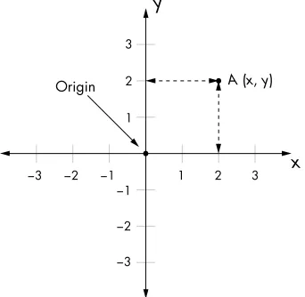
Now consider two number lines arranged as shown in Figure 2-2. The number lines intersect at right angles to each other and cross at the 0 point of each line. This forms a Cartesian coordinate plane, or an x-y plane, with the horizontal number line called the x-axis and the vertical line called the y-axis.
y
x 3
−3 −2 −1 3
2
1
1 2
−3 −2 −1
A (x, y) Origin
Figure 2-2: The Cartesian coordinate plane
As shown in Figure 2-2, x is the distance of the point from the origin along the x-axis, and y is the distance along the y-axis. The point where the two axes intersect is called the origin and has the coordinates (0, 0).
The Cartesian coordinate plane allows us to visualize the relationship between two sets of numbers. Here, I use the term set loosely to mean a col-lection of numbers. (We’ll learn about mathematical sets and how to work with them in Python in Chapter 5.) No matter what the two sets of numbers represent—temperature, baseball scores, or class test scores—all you need are the numbers themselves. Then, you can plot them—either on graph paper or on your computer with a program written in Python. For the rest of this book, I’ll use the term plot as a verb to describe the act of plotting two sets of numbers and the term graph to describe the result—a line, curve, or simply a set of points on the Cartesian plane.
Working with Lists and Tuples
As we make graphs with Python, we’ll work with lists and tuples. In Python, these are two different ways to store groups of values. Tuples and lists are very similar for the most part, with one major difference: after you create a list, it’s possible to add values to it and to change the order of the values. The values in a tuple, on the other hand, are immediately fixed and can’t be changed. We’ll use lists to store x- and y-coordinates for the points we want to plot. Tuples will come up in “Customizing Graphs” on page 41 when we learn to customize the range of our graphs. First, let’s go over some features of lists.
You can create a list by entering values, separated by commas, between square brackets. The following statement creates a list and uses the label
simplelist to refer to it:
>>> simplelist = [1, 2, 3]
Now you can refer to the individual numbers—1, 2, and 3—using the label and the position of the number in the list, which is called the index. So simplelist[0] refers to the first number, simplelist[1] refers to the second number, and simplelist[2] refers to the third number:
>>> simplelist[0]
1
>>> simplelist[1]
2
>>> simplelist[2]
3
Lists can store strings, too:
>>> stringlist = ['a string','b string','c string']
>>> stringlist[0]
One advantage of creating a list is that you don’t have to create a separate label for each value; you just create a label for the list and use the index posi-tion to refer to each item. Also, you can add to the list whenever you need to store new values, so a list is the best choice for storing data if you don’t know beforehand how many numbers or strings you may need to store.
An empty list is just that—a list with no items or elements—and it can be created like this:
>>> emptylist = []
Empty lists are mainly useful when you don’t know any of the items that will be in your list beforehand but plan to fill in values during the execu-tion of a program. In that case, you can create an empty list and then use the append() method to add items later:
u >>> emptylist just one way of adding values to a list. There are others, but we won’t need them for this chapter.
Creating a tuple is similar to creating a list, but instead of square brackets, you use parentheses:
>>> simpletuple = (1, 2, 3)
You can refer to an individual number in simpletuple using the corre-sponding index in brackets, just as with lists:
>>> simpletuple[0]
>>> simpletuple[1]
2
>>> simpletuple[2]
3
You can also use negative indices with both lists and tuples. For example,
simplelist[-1] and simpletuple[-1] would refer to the last element of the list or the tuple, simplelist[-2] and simpletuple[-2] would refer to the second-to-last element, and so on.
Tuples, like lists, can have strings as values, and you can create an empty tuple with no elements as emptytuple=(). However, there’s no append() method to add a new value to an existing tuple, so you can’t add values to an empty tuple. Once you create a tuple, the contents of the tuple can’t be changed.
Iterating over a List or Tuple
We can go over a list or tuple using a for loop as follows:
>>> l = [1, 2, 3]
>>> for item in l: print(item)
This will print the items in the list:
1 2 3
The items in a tuple can be retrieved in the same way.
Sometimes you might need to know the position or the index of an item in a list or tuple. You can use the enumerate() function to iterate over all the items of a list and return the index of an item as well as the item itself. We use the labels index and item to refer to them:
>>> l = [1, 2, 3]
>>> for index, item in enumerate(l): print(index, item)
This will produce the following output:
0 1 1 2 2 3
Creating Graphs with Matplotlib
We’ll be using matplotlib to make graphs with Python. Matplotlib is a Python package, which means that it’s a collection of modules with related functionality. In this case, the modules are useful for plotting numbers and making graphs. Matplotlib doesn’t come built in with Python’s stan-dard library, so you’ll have to install it. The installation instructions are covered in Appendix A. Once you have it installed, start a Python shell. As explained in the installation instructions, you can either continue using IDLE shell or use Python’s built-in shell.
Now we’re ready to create our first graph. We’ll start with a simple graph with just three points: (1, 2), (2, 4), and (3, 6). To create this graph, we’ll first make two lists of numbers—one storing the values of the x-coordinates of these points and another storing the y-coordinates. The following two state-ments do exactly that, creating the two lists x_numbers and y_numbers:
>>> x_numbers = [1, 2, 3]
>>> y_numbers = [2, 4, 6]
From here, we can create the plot:
>>> from pylab import plot, show
>>> plot(x_numbers, y_numbers)
[<matplotlib.lines.Line2D object at 0x7f83ac60df10>]
In the first line, we import the plot() and show() functions from the pylab
module, which is part of the matplotlib package. Next, we call the plot() func-tion in the second line. The first argument to the plot() function is the list of numbers we want to plot on the x-axis, and the second argument is the cor-responding list of numbers we want to plot on the y-axis. The plot() function returns an object—or more precisely, a list containing an object. This object contains the information about the graph that we asked Python to create. At this stage, you can add more information, such as a title, to the graph, or you can just display the graph as it is. For now we’ll just display the graph.
The plot() function only creates the graph. To actually display it, we have to call the show() function:
>>> show()
Figure 2-3: A graph showing a line passing through the points (1, 2), (2, 4), and (3, 6)
Notice that instead of starting from the origin (0, 0), the x-axis starts from the number 1 and the y-axis starts from the number 2. These are the lowest numbers from each of the two lists. Also, you can see incre-ments marked on each of the axes (such as 2.5, 3.0, 3.5, etc., on the y-axis). In “Customizing Graphs” on page 41, we’ll learn how to control those aspects of the graph, along with how to add axes labels and a graph title.
You’ll notice in the interactive shell that you can’t enter any further statements until you close the matplotlib window. Close the graph window so that you can continue programming.
Marking Points on Your Graph
If you want the graph to mark the points that you supplied for plotting, you can use an additional keyword argument while calling the plot() function:
By entering marker='o', we tell Python to mark each point from our lists with a small dot that looks like an o. Once you enter show() again, you’ll see that each point is marked with a dot (see Figure 2-4).
Figure 2-4: A graph showing a line passing through the points (1, 2), (2, 4), and (3, 6) with the points marked by a dot
The marker at (2, 4) is easily visible, while the others are hidden in the very corners of the graph. You can choose from several marker options, including 'o', '*', 'x', and '+'. Using marker= includes a line connecting the points (this is the default). You can also make a graph that marks only the points that you specified, without any line connecting them, by omitting marker=:
>>> plot(x_numbers, y_numbers, 'o')
[<matplotlib.lines.Line2D object at 0x7f2549bc0bd0>]
Figure 2-5: A graph showing the points (1, 2), (2, 4), and (3, 6)
As you can see, only the points are now shown on the graph, with no line connecting them. As in the previous graph, the first and the last points are barely visible, but we’ll soon see how to change that.
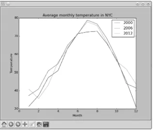
Graphing the Average Annual Temperature in New York City
Let’s take a look at a slightly larger set of data so we can explore more fea-tures of matplotlib. The average annual temperafea-tures for New York City— measured at Central Park, specifically—during the years 2000 to 2012 are as follows: 53.9, 56.3, 56.4, 53.4, 54.5, 55.8, 56.8, 55.0, 55.3, 54.0, 56.7, 56.4, and 57.3 degrees Fahrenheit. Right now, that just looks like a random jumble of numbers, but we can plot this set of temperatures on a graph to make the rise and fall in the average temperature from year to year much clearer:
>>> nyc_temp = [53.9, 56.3, 56.4, 53.4, 54.5, 55.8, 56.8, 55.0, 55.3, 54.0, 56.7, 56.4, 57.3]
>>> plot(nyc_temp, marker='o')
We store the average temperatures in a list, nyc_temp. Then, we call the function plot() passing only this list (and the marker string). When you use plot() on a single list, those numbers are automatically plotted on the y-axis. The corresponding values on the x-axis are filled in as the positions of each value in the list. That is, the first temperature value, 53.9, gets a cor-responding x-axis value of 0 because it’s in position 0 of the list (remember, the list position starts counting from 0, not 1). As a result, the numbers plotted on the x-axis are the integers from 0 to 12, which we can think of as corresponding to the 13 years for which we have temperature data.
Enter show() to display the graph, which is shown in Figure 2-6. The graph shows that the average temperature has risen and fallen from year to year. If you glance at the numbers we plotted, they really aren’t very far apart from each other. However, the graph makes the variations seem rather dramatic. So, what’s going on? The reason is that matplotlib chooses the range of the y-axis so that it’s just enough to enclose the data supplied for plotting. So in this graph, the y-axis starts at 53.0 and its highest value is 57.5. This makes even small differences look magnified because the range of the y-axis is so small. We’ll learn how to control the range of each axis in “Customizing Graphs” on page 41.
You can also see that numbers on the y-axis are floating point numbers (because that’s what we asked to be plotted) and those on the x-axis are integers. Matplotlib can handle either.
Plotting the temperature without showing the corresponding years is a quick and easy way to visualize the variations between the years. If you were planning to present this graph to someone, however, you’d want to make it clearer by showing which year each temperature corresponds to. We can easily do this by creating another list with the years in it and then calling the plot() function:
>>> nyc_temp = [53.9, 56.3, 56.4, 53.4, 54.5, 55.8, 56.8, 55.0, 55.3, 54.0, 56.7, 56.4, 57.3]
>>> years = range(2000, 2013)
>>> plot(years, nyc_temp, marker='o')
[<matplotlib.lines.Line2D object at 0x7f2549a616d0>] >>> show()
We use the range() function we learned about in Chapter 1 to specify the years 2000 to 2012. Now you’ll see the years displayed on the x-axis (see Figure 2-7).