Table of Contents
1.3 Equiprobable Outcome Spaces and De Méré's Problem 1.4 Probabilities for Compound Events
2.5 Utility Functions and Rational Choice Theory 2.6 Limitations of Rational Choice Theory
4.2 Sharing Profits: De Méré's Second Problem 4.3 Exercises
5.1 The Monty Hall Paradox
7.3 How Long will My Money Last? 7.4 Is This Wheel Biased?
8.3 A Gambling System that Works: Card Counting 8.4 Exercises
Chapter 9: Poker 9.1 Basic Rules
9.2 Variants of Poker 9.3 Additional Rules
9.4 Probabilities of Hands in Draw Poker 9.5 Probabilities of Hands in Texas Hold'em 9.6 Exercises
Chapter 10: Strategic Zero-Sum Games with Perfect Information 10.1 Games with Dominant Strategies
10.2 Solving Games with Dominant and Dominated Strategies 10.3 General Solutions for Two Person Zero-Sum Games
10.4 Exercises
Chapter 11: Rock–Paper–Scissors: Mixed Strategies in Zero-Sum Games 11.1 Finding Mixed-Strategy Equilibria
11.3 Bluffing as a Strategic Game with a Mixed-Strategy Equilibrium 11.4 Exercises
Chapter 12: The Prisoner's Dilemma and Other Strategic Non-zero-sum Games 12.1 The Prisoner's Dilemma
12.2 The Impact of Communication and Agreements 12.3 Which Equilibrium?
12.4 Asymmetric Games 12.5 Exercises
Chapter 13: Tic-Tac-Toe and Other Sequential Games of Perfect Information 13.1 The Centipede Game
13.2 Tic-Tac-Toe
13.3 The Game of Nim and the First- and Second-Mover Advantages 13.4 Can Sequential Games be Fun?
13.5 The Diplomacy Game 13.6 Exercises
Appendix A: A Brief Introduction to R A.1 Installing R
A.11 Other Things to Keep in Mind Index
End User License Agreement
List of Illustrations
Chapter 1: An Introduction to Probability
Figure 1.2 Venn diagram for the (a) union and (b) intersection of two events. Figure 1.3 Venn diagram for the addition rule.
Chapter 2: Expectations and Fair Values
Figure 2.1 Running profits from a wager that costs $1 to join and pays nothing if a coin comes up tails and $1.50 if the coin comes up tails (solid line). The gray
horizontal line corresponds to the expected profit.
Figure 2.2 Running profits from Wagers 1 (continuous line) and 2 (dashed line). Figure 2.3 Running profits from Wagers 3 (continuous line) and 4 (dashed line).
Chapter 3: Roulette
Figure 3.1 The wheel in the French/European (left) and American (right) roulette and respective areas of the roulette table where bets are placed.
Figure 3.2 Running profits from a color (solid line) and straight-up (dashed line) bet.
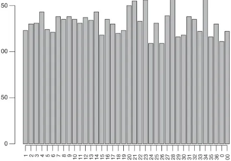
Figure 3.3 Empirical frequency of each pocket in 5000 spins of a biased wheel. Figure 3.4 Cumulative empirical frequency for a single pocket in an unbiased wheel.
Chapter 5: The Monty Hall Paradox and Conditional Probabilities
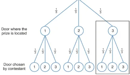
Figure 5.1 Each branch in this tree represents a different decision and the s represent the probability of each door being selected to contain the prize.
Figure 5.2 The tree structure now represents an extra level, representing the contestant decisions and the probability for each decision to be the one chosen. Figure 5.3 Decision tree for the point when Monty decides which door to open assuming the prize is behind door 3.
Figure 5.4 Partitioning the event space.
Figure 5.5 Tree representation of the outcomes of the game of urns under the
optimal strategy that calls yellow balls as coming from Urn 3 and blue and red balls as coming from urn 2.
Chapter 6: Craps
Figure 6.1 The layout of a craps table.
Figure 6.2 Tree representation for the possible results of the game of craps. Outcomes that lead to the pass line bet winning are marked with W, while those that lead to a lose are marked L.
Figure 6.4 Tree representation for the possible results of the game of craps with the probabilities for all scenarios.
Chapter 7: Roulette Revisited
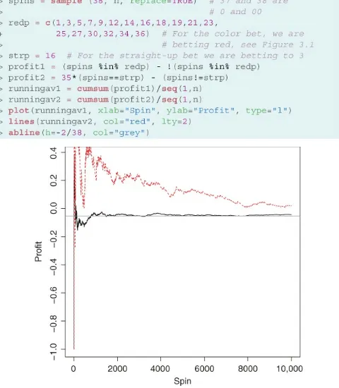
Figure 7.1 The solid line represents the running profits from a martingale doubling system with $1 initial wagers for an even bet in roulette. The dashed horizontal line indicates the zero-profit level.
Figure 7.2 Running profits from a Labouchère system with an initial list of $50 entries of $10 for an even bet in roulette. Note that the simulation stops when the cumulative profit is ; the number of spins necessary to reach this number will vary from simulation to simulation.
Figure 7.3 Running profits over 10,000 spins from a D'Alembert system with an initial bet of $5, change in bets of $1, minimum bet of $1 and maximum bet of $20 to an even roulette bet.
Chapter 8: Blackjack
Figure 8.1 A 52-card French-style deck.
Chapter 9: Poker
Figure 9.1 Examples of poker hands.
Chapter 11: Rock–Paper–Scissors: Mixed Strategies in Zero-Sum Games
Figure 11.1 Graphical representation of decisions in a simplified version of poker.
Chapter 12: The Prisoner's Dilemma and Other Strategic Non-zero-sum Games
Figure 12.1 Expected utilities for Ileena (solid line) and Hans (dashed line) in the game of chicken as function of the probability that Hans will swerve with
probability if we assume that Ileena swerves with probability .
Figure 12.2 Expected utilities for Ileena (solid line) and Hans (dashed line) in the game of chicken as function of the probability that Ileena will swerve with
probability if we assume that Hans swerves with probability .
Figure 12.3 Expected utilities for Ileena (solid line) and Hans (dashed line) in the game of chicken as function of the probability that Hans will swerve with
probability if we assume that Ileena always swerves.
Chapter 13: Tic-Tac-Toe and Other Sequential Games of Perfect Information
Figure 13.1 Extensive-form representation of the centipede game.
Figure 13.2 Reduced extensive-form representation of the centipede game after solving for Carissa's optimal decision during the third round of play.
optimal decision during the third round of play.
Figure 13.4 A game of tic-tac-toe where the player represented by X plays first and the player represented by O wins the game. The boards should be read left to right and then top to bottom.
Figure 13.5 A small subsection of the extensive-form representation of tic-tac-toe. Figure 13.6 Examples of boards in which the player using the X mark created a fork for themselves, a situation that should be avoided by their opponent. In the left figure, player 1 (who is using the X) claimed the top left corner in their first move, then player 2 claimed the top right corner, player 1 responded by claiming the bottom right corner, which forces player 2 to claim the center square (in order to block a win), and player 1 claims the bottom left corner too. At this point, player 1 has created a fork since they can win by placing a mark on either of the cells
marked with an F. Similarly, in the right Figure player 1 claimed the top left corner, player 2 responded by claiming the bottom edge square, then player 1 took the
center square, which forced player 2 to take the bottom right corner to block a win. After that, if player 1 places their mark on the bottom left corner they would have created a fork.
Figure 13.7 Extended-form representation of the game of Nim with four initial pieces.
Figure 13.8 Pruned tree for a game of Nim with four initial pieces after the optimal strategy at the third round has been elucidated.
Figure 13.9 Pruned tree for a game of Nim with four initial pieces after the optimal strategy at the second round has been elucidated.
Figure 13.10 The diplomacy game in extensive form.
Figure 13.11 First branches pruned in the diplomacy game. Figure 13.12 Pruned tree associated with the diplomacy game.
Appendix A: A Brief Introduction to R
Figure A.1 The R interactive command console in a Mac OS X computer. The symbol > is a prompt for users to provide instructions; these will be executed immediately after the user presses the RETURN key.
Figure A.2 A representation of a vector x of length 6 as a series of containers, each one of them corresponding to a different number.
Figure A.3 An example of a scatterplot in R]An example of a scatterplot in R. Figure A.4 An example of a line plot in R.
List of Tables
Chapter 1: An Introduction to Probability
Table 1.1 Two different ways to think about the outcome space associated with rolling two dice
Chapter 2: Expectations and Fair Values
Table 2.1 Winnings for the different lotteries in Allais paradox
Table 2.2 Winnings for 11% of the time for the different lotteries in Allais paradox
Chapter 3: Roulette
Table 3.1 Inside bets for the American wheel Table 3.2 Outside bets for the American wheel
Table 3.3 Outcomes of a combined bet of $2 on red and $1 on the second dozen
Chapter 4: Lotto and Combinatorial Numbers
Table 4.1 List of possible groups of 3 out of 6 numbers, if the order of the numbers is not important
Chapter 5: The Monty Hall Paradox and Conditional Probabilities
Table 5.1 Probabilities of winning if the contestant in the Monty problem switches doors
Table 5.2 Studying the relationship between smoking and lung cancer
Chapter 6: Craps
Table 6.1 Names associated with different combinations of dice in craps
Table 6.2 All possible equiprobable outcomes associated with two dice being rolled Table 6.3 Sum of points associated with the roll of two dice
Chapter 7: Roulette Revisited
Table 7.1 Accumulated losses from playing a martingale doubling system with an initial bet of $1 and an initial bankroll of $1000
Table 7.2 Probability that you play exactly rounds before you lose your first dollar for between 1 and 6
Chapter 8: Blackjack
Table 8.1 Probability of different hands assuming that the house stays on all 17s and that the game is being played with a large number of decks
Table 8.3 Optimal splitting strategy
Table 8.4 Probability of different hands assuming that the house stays on all 17s and that the game is being played with a single deck where all Aces, 2s, 3s, 4s, 5s, and 6s have been removed
Table 8.5 Probability of different hands assuming that the house stays on all 17s, conditional on the face-up card
Chapter 9: Poker
Table 9.1 List of poker hands
Table 9.2 List of opponent's poker hands that can beat our two-pair
Chapter 10: Strategic Zero-Sum Games with Perfect Information
Table 10.1 Profits in the game between Pevier and Errian Table 10.2 Poll results for Matt versus Ling (first scenario) Table 10.3 Best responses for Matt (first scenario)
Table 10.4 Best responses for Ling (first scenario)
Table 10.5 Poll results for Matt versus Ling (second scenario) Table 10.6 Best responses for Matt (second scenario)
Table 10.7 Best responses for Ling (second scenario)
Table 10.8 Poll results for Matt versus Ling (third scenario) Table 10.9 Best responses for Ling (third scenario)
Table 10.10 Best responses for Matt (third scenario)
Table 10.11 Reduced Table for poll results for Matt versus Ling Table 10.12 A game without dominant or dominated strategies
Table 10.13 Best responses for Player 1 in our game without dominant or dominated strategies
Table 10.14 Best responses for Player 2 in our game without dominant or dominated strategies
Table 10.15 Example of a game with multiple equilibria
Chapter 11: Rock–Paper–Scissors: Mixed Strategies in Zero-Sum Games
Table 11.1 Player's profit in rock–paper–scissors
and scissors with probability
Table 11.4 Utilities associated with different penalty kick decisions
Table 11.5 Utility associated with different actions taken by the kicker if he
assumes that goal keeper selects left with probability , center with probability , and right with probability
Table 11.6 Expected profits in the simplified poker
Table 11.7 Best responses for you in the simplified poker game Table 11.8 Best responses for Alya in the simplified poker game
Table 11.9 Expected profits in the simplified poker game after eliminating dominated strategies
Table 11.10 Expected profits associated with different actions you take if you assume that Alya will select with probability and with probability
Chapter 12: The Prisoner's Dilemma and Other Strategic Non-zero-sum Games
Table 12.1 Payoffs for the prisoner's dilemma
Table 12.2 Best responses for Prisoner 2 in the prisoner's dilemma game Table 12.3 Communication game in normal form
Table 12.4 Best responses for Anastasiya in the communication game Table 12.5 Best responses for Anil in the communication game
Table 12.6 Expected utility for Anil in the communication game Table 12.7 The game of chicken
Table 12.8 Best responses for Ileena in the game of chicken Table 12.9 Expected utility for Ileena in the game of chicken Table 12.10 A fictional game of swords in Star Wars
Table 12.11 Best responses for Ki-Adi in the sword game Table 12.12 Best responses for Asajj in the sword game
Probability, Decisions and Games
A Gentle Introduction using R
This edition first published 2018 © 2018 John Wiley & Sons, Inc.
All rights reserved. No part of this publication may be reproduced, stored in a retrieval system, or transmitted, in any form or by any means, electronic, mechanical, photocopying, recording or otherwise, except as permitted by law. Advice on how to obtain permission to reuse material from this title is available at http://www.wiley.com/go/permissions. The right of Abel Rodríguez and Bruno Mendes to be identified as the authors of this work has been asserted in accordance with law.
Registered Offices
John Wiley & Sons, Inc., 111 River Street, Hoboken, NJ 07030, USA
Editorial Office
111 River Street, Hoboken, NJ 07030, USA
For details of our global editorial offices, customer services, and more information about Wiley products visit us at www.wiley.com.
Wiley also publishes its books in a variety of electronic formats and by print-on-demand. Some content that appears in standard print versions of this book may not be available in other formats.
Limit of Liability/Disclaimer of Warranty
The publisher and the authors make no representations or warranties with respect to the accuracy or completeness of the contents of this work and specifically disclaim all warranties; including without limitation any implied warranties of fitness for a particular purpose. This work is sold with the understanding that the publisher is not engaged in rendering professional services. The advice and strategies contained herein may not be suitable for every situation. In view of on-going research, equipment modifications, changes in governmental regulations, and the constant flow of information relating to the use of experimental reagents, equipment, and devices, the reader is urged to review and evaluate the information provided in the package insert or instructions for each chemical, piece of equipment, reagent, or device for, among other things, any changes in the instructions or indication of usage and for added warnings and precautions. The fact that an organization or website is referred to in this work as a citation and/or potential source of further information does not mean that the author or the publisher endorses the information the organization or website may provide or recommendations it may make. Further, readers should be aware that websites listed in this work may have changed or disappeared between when this works was written and when it is read. No warranty may be created or extended by any promotional statements for this work. Neither the publisher nor the author shall be liable for any damages arising here from.
Library of Congress Cataloging-in-Publication Data:
Names: Rodríguez, Abel, 1975- author. | Mendes, Bruno, 1970- author.
Title: Probability, decisions, and games : a gentle introduction using R / by Abel Rodríguez, Bruno Mendes. Description: Hoboken, NJ : Wiley, 2018. | Includes index. |
Identifiers: LCCN 2017047636 (print) | LCCN 2017059013 (ebook) | ISBN 9781119302612 (pdf) | ISBN 9781119302629 (epub) | ISBN 9781119302605 (pbk.)
Subjects: LCSH: Game theory-Textbooks. | Game theory-Data processing. | Statistical decision-Textbooks. | Statistical decision-Data processing. | Probabilities--Textbooks. | Probabilities-Data processing. | R (Computer program language) Classification: LCC QA269 (ebook) | LCC QA269 .R63 2018 (print) | DDC 519.30285/5133-dc23
LC record available at https://lccn.loc.gov/2017047636 Cover design: Wiley
To Sabrina Abel
Preface
Why Gambling and Gaming?
Games are a universal part of human experience and are present in almost every culture; the earliest games known (such as senet in Egypt or the Royal Game of Ur in Iraq) date back to at least 2600 B.C. Games are characterized by a set of rules regulating the
behavior of players and by a set of challenges faced by those players, which might involve a monetary or nonmonetary wager. Indeed, the history of gaming is inextricably linked to the history of gambling, and both have played an important role in the development of modern society.
Games have also played a very important role in the development of modern
mathematical methods, and they provide a natural framework to introduce simple
concepts that have wide applicability in real-life problems. From the point of view of the mathematical tools used for their analysis, games can be broadly divided between random games and strategic games. Random games pit one or more players against “nature” that is, an unintelligent opponent whose acts cannot be predicted with certainty. Roulette is the quintessential example of a random game. On the other hand, strategic games pit two or more intelligent players against each other; the challenge is for one player to outwit their opponents. Strategic games are often subdivided into simultaneous (e.g., rock– paper–scissors) and sequential (e.g., chess, tic-tac-toe) games, depending on the order in which the players take their actions. However, these categories are not mutually
exclusive; most modern games involve aspects of both strategic and random games. For example, poker incorporates elements of random games (cards are dealt at random) with those of a sequential strategic game (betting is made in rounds and “bluffing” can win you a game even if your cards are worse than those of your opponent).
One of the key ideas behind the mathematical analysis of games is the rationality
often means evaluating the alternatives available to other players and finding a “best response” to them. This is often taken to mean minimizing losses, but the two concepts are not necessarily identical. Indeed, one important insight gleaned from game theory (the area of mathematics that studies strategic games) is that optimal strategies for zero-sum games (i.e., those games where a player can win only if another loses the same
amount) and non zero-sum games can be very different. Also, it is important to highlight that randomness plays a role even in purely strategic games. An excellent example is the game of rock–paper–scissors. In principle, there is nothing inherently random in the rules of this game. However, the optimal strategy for any given player is to select his or her move uniformly at random among the three possible options that give the game its name.
The mathematical concepts underlying the analysis of games and gambles have practical applications in all realms of science. Take for example the game of blackjack. When you play blackjack, you need to sequentially decide whether to hit (i.e., get an extra card), stay (i.e., stop receiving cards) or, when appropriate, double down, split, or surrender.
Optimally playing the game means that these decisions must be taken not only on the basis of the cards you have in your hand but also on the basis of the cards shown by the dealer and all other players. A similar problem arises in the diagnosis and treatment of medical conditions. A doctor has access to a series of diagnostic tests and treatment options; decisions on which one is to be used next needs to be taken sequentially based on the outcomes of previous tests or treatments for this as well as other patients. Poker provides another interesting example. As any experienced player can attest, bluffing is one of the most important parts of the game. The same rules that can be used to decide how to optimally bluff in poker can also be used to design optimal auctions that allow the auctioneer to extract the highest value assigned by the bidders to the object begin
auctioned. These strategies are used by companies such as Google and Yahoo to allocate advertising spots.
Using this Book
The goal of this book is to introduce basic concepts of probability, statistics, decision theory, and game theory using games. The material should be suitable for a college-level general education course for undergraduate college students who have taken an algebra or pre-algebra class. In our experience, motivated high-school students who have taken an algebra course should also be capable of handling the material.
The book is organized into 13 chapters, with about half focusing on general concepts that are illustrated using a wide variety of games, and about half focusing specifically on well-known casino games. More specifically, the first two chapters of the book are dedicated to a basic discussion of utility and probability theory in finite, discrete spaces. Then we move to a discussion of five popular casino games: roulette, lotto, craps, blackjack, and poker. Roulette, which is one of the simplest casino games to play and analyze, is used to
counting rules and the notions of permutations and combinatorial numbers that allow us to compute probabilities in large equiprobable spaces. The games of craps and blackjack are used to illustrate and develop conditional probabilities. Finally, the discussion of
poker is helpful to illustrate how many of the ideas from previous chapters fit in together. The last four chapters of the book are dedicated to game theory and strategic games. Since this book is meant to support a general education course, we restrict attention to
simultaneous and sequential games of perfect information and avoid games of imperfect information.
The book uses computer simulations to illustrate complex concepts and convince
students that the calculations presented in the book are correct. Computer simulations have become a key tool in many areas of scientific inquiry, and we believe that it is important for students to experience how easy access to computing power has changed science over the last 25 years. During the development of the book, we experimented with using spreadsheets but decided that they did not provide enough flexibility. In the end we settled for using R (https://www.r-project.org). R is an interactive environment that allows users to easily implement simple simulations even if they have limited experience with programming. To facilitate its use, we have included an overview and introduction to the R in Appendix A, as well as sidebars in each chapter that introduces features of the
language that are relevant for the examples discussed in them. With a little extra work, this book could be used as the basis for a course that introduces students to both
probability/statistics and programming. Alternatively, the book can also be read while ignoring the R commands and focusing only on the graphs and other output generated by it.
In the past, we have paired the content of this book with screenings of movies from History Channel's Breaking Vegas series. We have found the movies Beat the Wheel, Roulette Attack, Dice Dominator, and Professor Blackjack (each approximately 45 min in length) particularly fitting. These movies are helpful in explaining the rules of the games and providing an entertaining illustration of basic concepts such as the law of large
numbers.
November 2017
Acknowledgments
We would like to thank all our colleagues, teaching assistants, and students who
About the Companion Website
This book is accompanied by a companion website:
www.wiley.com/go/Rodriguez/Probability_Decisions_and_Games
Student Website contains:
Chapter 1
An Introduction to Probability
The study of probability started in the seventeenth century when Antoine Gambaud (who called himself the “Chevalier” de Méré) reached out to the French mathematician Blaise Pascal for an explanation of his gambling loses. De Méré would commonly bet that he could get at least one ace when rolling 4 six-sided dice, and he regularly made money on this bet. When that game started to get old, he started betting on getting at least one double-one in 24 rolls of two dice. Suddenly, he was losing money!
De Méré was dumbfounded. He reasoned that two aces in two rolls are 1/6 as likely as one ace in one roll. To compensate for this lower probability, the two dice should be rolled six times. Finally, to achieve the probability of one ace in four rolls, the number of the rolls should be increased fourfold (to 24). Therefore, you would expect a couple of aces to turn up in 24 double rolls with the same frequency as an ace in four single rolls. As you will see in a minute, although the very first statement is correct, the rest of his argument is not!
1.1 What is Probability?
Let's start by establishing some common language. For our purposes, an experiment is any action whose outcome cannot necessarily be predicted with certainty; simple
examples include the roll of a die and the card drawn from a well-shuffled deck. The outcome space of an experiment is the set of all possible outcomes associated with it; in the case of a die, it is the set , while for the card drawn from a deck, the outcome space has 52 elements corresponding to all combinations of 13 numbers (A, 2, 3, 4, 5, 6, 7, 8, 9, 10, J, Q, K) with four suits (hearts, diamonds, clubs, and spades):
while the probability associated with these events is denoted by and . By
definition, the probability of at least one event in the outcome space happening is 1, and therefore the sum of the probabilities associated with each of the outcomes also has to be equal to 1. On the other hand, the probability of an event not happening is simply the complement of the probability of the event happening, that is,
where should be read as “ not happening” or “not .” For example, if
, then .
There are a number of ways in which a probability can be interpreted. Intuitively almost everyone can understand the concept of how likely something is to happen. For instance, everyone will agree on the meaning of statements such as “it is very unlikely to rain
tomorrow” or “it is very likely that the LA Lakers will win their next game.” Problems arise when we try to be more precise and quantify (i.e., put into numbers) how likely the event is to occur. Mathematicians usually use two different interpretations of probability, which are often called the frequentist and subjective interpretations.
The frequentist interpretation is used in situations where the experiment in question can be reproduced as many times as desired. Relevant examples for us include rolling a die, drawing cards from a well shuffled deck, or spinning the roulette wheel. In that case, we can think about repeating the experiment a large number of times (call it ) and
recording how many of them result in outcome (call it ). The probability of the
event can be defined by thinking about what happens to the ratio (sometimes called the empirical frequency) as grows.
For example, let . We often assign this event a
probability of 1/2, that is, we let . This is often argued on the
Sidebar 1.1 Random sampling in
R
R provides easy-to-use functions to simulate the results of random experiments. When working with discrete outcome spaces such as those that appear with most casino and tabletop games, the function sample() is particularly useful. The first argument of sample() is a vector whose entries correspond to the elements of the outcome space, the second is the number of samples that we are interested in
drawing, and the third indicates whether sampling will be performed with or without replacement (for now we are only drawing with replacement).
Similarly, if we want to roll a six-sided die 15 times:
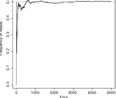
basis of symmetry: there is no apparent reason why one side of a regular coin would be more likely to come up than the other. Since you can flip a coin as many times as you want, the frequentist interpretation of probability can be used to interpret the value 1/2. Because flipping the coin by hand is very time-consuming, we instead use a computer to simulate 5000 flips of a coin and plot the cumulative empirical frequency of heads using the following R code (please see Sidebar 1.1 for details on how to simulate random
Figure 1.1 Cumulative empirical frequency of heads (black line) in 5000 simulated flips of a fair coin. The gray horizontal line corresponds to the true probability .
Note that the empirical frequency fluctuates, particularly when you have flipped the coin just a few times. However, as the number of flips ( in our formula) becomes larger and larger, the empirical frequency gets closer and closer to the “true” probability and fluctuates less and less around it.
The convergence of the empirical frequency to the true probability of an event is captured by the so-called law of large numbers.
Law of Large Numbers for Probabilities
Let represent the number of times that event A happens in a total of n identical repetitions of an experiment, and let denote the probability of event A. Then
approaches as n grows.
Even though the frequency interpretation of probability we just described is appealing, it cannot be applied to situations where the experiment cannot be repeated. For example, consider the event
There will be only one tomorrow, so we will only get to observe the “experiment”
(whether it rains or not) once. In spite of that, we can still assign a probability to based on our knowledge of the season, today's weather, and our prior experience of what that implies for the weather tomorrow. In this case, corresponds to our “degree of belief” on tomorrow's rain. This is a subjective probability, in the sense that two reasonable
people might not necessarily agree on the number.
To summarize, although it is easy for us to qualitatively say how likely some event is to happen, it is very challenging if we try to put a number to it. There are a couple of ways in which we can think about this number:
The frequentist interpretation of probability that is useful when we can repeat and observe an experiment as many times as we want.
The subjective interpretation of probability, which is useful in almost any probability experiment where we can make a judgment of how likely an event is to happen, even if the experiment cannot be repeated.
1.2 Odds and Probabilities
In casinos and gambling dens, it is very common to express the probability of events in the form of odds (either in favor or against). The odds in favor of an event is simply the ratio of the probability of that event happening divided by the probability of the event not happening, that is,
Similarly, the odds against are simply the reciprocal of the odds in favor, that is,
In the context of casino games, the odds we have just discussed are sometimes called the winning odds (or the losing odds). In that context, you will also hear sometimes about payoff odds. This is a bit of a misnomer, as these represent the ratio of payoffs, rather than the ratio of probabilities.
For example, the winning odds in favor of any given number in American roulette are 1 to 37, but the payoff odds for the same number are just 1 to 35 (which means that, if you win, every dollar you bet will bring back $35 in profit). This distinction is important, as many of the odds on display in casinos refer to these payoff odds rather than the winning odds. Keep this in mind!
1.3 Equiprobable Outcome Spaces and De Méré's Problem
In many problems, we can use symmetry arguments to come up with reasonable values for the probability of simple events. For example, consider a very simple experiment
consisting of rolling a perfect, six-sided (cubic) die. This type of dice typically has its sides marked with the numbers 1–6. We could ask about the probability that a specific number (say, 3) comes up on top. Since the six sides are the only possible outcomes (we discount the possibility of the die resting on edges or vertexes!) and they are symmetric with
respect to each other, there is no reason to think that one is more likely to come up than another. Therefore, it is natural to assign probability 1/6 to each side of the die.
Outcome spaces where all outcomes are assumed to have the same probability (such as the outcome space associated with the roll of a six-sided die) are called equiprobable spaces. In equiprobable spaces, the probabilities of different events can be computed using a simple formula:
Note the similarities with the law of large numbers and the frequentist interpretation of probability.
Although the concept of equiprobable spaces is very simple, some care needs to be
exercised when applying the formula. Let's go back to Chevalier de Méré's predicament. Recall that De Méré would commonly bet that he could get at least one ace when rolling 4 (fair) six-sided dice, and he would regularly make money on this bet. To make the game more interesting, he started betting on getting at least one double-one in 24 rolls of two dice, after which he started to lose money.
can be used in this case, so it is natural to think of this outcome space as equiprobable. However, there are two ways in which we could construct the outcome space, depending on whether we consider the order of the dice relevant or not (see Table 1.1). The first construction leads to the conclusion that getting a double one has probability
, while the second leads to a probability of . The
question is, which one is the correct one?
Table 1.1 Two different ways to think about the outcome space associated with rolling two dice
Order is irrelevant 21 outcomes in total Order is relevant 36 outcomes in total
1–1 2–2 3–3 4–4 5–5 6–6 1–1 2–1 3–1 4–1 5–1 6–1
In order to gain some intuition, let's run another simulation in R in which two dice are rolled 100,000 times each.[
The result of the simulation is very close to , which suggests that this is the right answer. A formal argument can be constructed by thinking of the dice as being rolled sequentially rather than simultaneously. Since there are 6 possible outcomes of the first roll and another 6 possible outcomes for the second one, there is a total of 36 combined outcomes. Since just 1 of these 36 outcomes corresponds to a pair of ones, our formula for the probability of events in equiprobable spaces leads to the probability of 2 ones being 1/36. Underlying this result is a simple principle that we will call the multiplication principle of counting,
Multiplication Principle for Counting
If events can each happen in ways then they can happen
together in ways.
probability of losing the bet and, because no ties are possible, then obtain the probability of winning the bet as
For the first bet, the multiplication rule implies that there are a total of
possible outcomes when we roll 4 six-sided dice. If we are patient enough, we can list all the possibilities:
On the other hand, since for each single die there are five outcomes that are not an ace, there are outcomes for which De Méré losses this bet. Again, we could
potentially enumerate these outcomes
The probability that De Méré wins his bet is therefore
You can corroborate this result with a simple simulation of 100,000 games:
equiprobable outcomes when you roll 2 six-sided dice, 35 of which are unfavorable to the bet. Therefore, there are possible outcomes when two dice are rolled together 24 times, of which are unfavorable to the player, and the probability of winning this bet is equal to
Again, you can verify the results of the calculation using a simulation:
The fact that the probability of winning is less than 0.5 explains why De Méré was losing money! Note, however, that if he had used 25 rolls instead of 24, then the probability of
winning would be , which would have made it a winning bet for De
Méré (but not as good as the original one!).
1.4 Probabilities for Compound Events
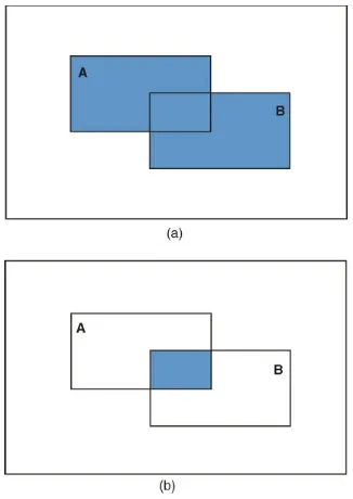
A compound event is an event that is created by aggregating two or more simple events. For example, we might want to know what is the probability that the number selected by the roulette is black or even, or what is the probability that we draw a card from the deck that is both a spade and a number.
As the examples above suggest, we are particularly interested in two types of operations to combine events. On the one hand, the union of two events and (denoted by
) corresponds to the event that happens if either or (or both) happen. On the other hand, the intersection of two events (denoted by ) corresponds to the event that happens only if both and happen simultaneously. The results from these operations can be represented graphically using a Venn diagram (see Figure 1.2) where the simple events and correspond to the rectangles. In Figure 1.2(a), the
combination of the areas of both rectangles corresponds to the union of the events. In
events cannot happen simultaneously), we say that the events are disjoint or mutually exclusive.
Figure 1.2 Venn diagram for the (a) union and (b) intersection of two events.
In many cases, the probabilities of compound events can be computed directly from the sample space by carefully counting favorable cases. However, in other cases, it is easier to compute them from simpler events. Just as there is a rule for probability of two events happening together, there is a second rule for the probability of two alternative events (e.g., the probability of obtaining an even number or a 2 when rolling a die), which is sometimes called the Addition Rule of probability:
For any two events,
Figure 1.3 presents a graphical representation of two events using Venn diagrams; it
provides some hints at why the formula takes this form. If we simply add and , the darker region (which corresponds to ) is counted twice. Hence, we need to subtract it once in order to get the right result. If two events are mutually exclusive (i.e.,
they cannot occur at the same time, which means that ), this formula
reduces to .
Similar rules can be constructed to compute the joint probability of two events, . For the time being, we will only present the simplified Multiplication Rule for the
probability of independent events. Roughly speaking, this rule is appropriate for when knowing that one of the events occur does not affect the probability that the other will occur.
For any two independent events,
In Chapter 5, we cover the concept of independent events in more detail and present more general rules to compute the joint probabilities.
1.5 Exercises
1. A man has 20 shirts and 10 ties. How many different shirt-and-tie combinations can he make?
2. If you have 5 different pants, 12 different shirts, and 3 pairs of shoes, how many days can you go without repeating the same outfit?
3. A fair six-sided die is rolled times and the number of rolls that turn out to be either a 1 or a 5, are recorded. From the law of large numbers, what is the
approximate value for that you expect to see?
are allowed, and no distinction is made between lower- and upper-case letters). How many distinct usernames are possible for the website?
5. Provide two examples of experiments for which the probability of the outcomes can only be interpreted from a subjective perspective. For each one of them, justify your choice and provide a value for such probability.
6. In how many ways can 13 students be lined up?
7. Re-write the following probability using the addition rule of probability: .
8. Re-write the following probability using the addition rule of probability: P(obtaining a total sum of 5 or an even sum when rolling a 2 six-sided dice).
9. Re-write the following probability using the rule of probability for complementary events: P(obtaining at least a 2 when rolling a six-sided die).
10. Re-write the following probability using the rule of probability for complementary events: P(obtaining at most a 5 when rolling a six-sided die).
11. Consider rolling a six-sided die. Which probability rule can be applied to the following probability
12. What is the probability of obtaining at least two heads when flipping a coin three times? Which probability rule was used in your reasoning?
13. Explain what is wrong with each of the following arguments.
a.
In 1 roll of a pair of six-sided dice, I have 1/36 of a chance to get a double ace. So in 24 rolls, I have of a chance to get at least one double ace.
14. What is the probability that, in a group of 30 people, at least two of them have the same birthday. Hint: Start by computing the probability that no two people have the same birthday.
Chapter 2
Expectations and Fair Values
Let's say that you are offered the following bet: you pay $1, then a coin is flipped. If the coin comes up tails you lose your money. On the other hand, if it comes up heads, you get back your dollar along with a 50 cents profit. Would you take it?
Your gut feeling probably tells you that this bet is unfair and you should not take it. As a matter of fact, in the long run, it is likely that you will lose more money than you could possibly make (because for every dollar you lose, you will only make a profit of 50 cents, and winning and losing have the same probability). The concept of mathematical
expectation allows us to generalize this observation to more complex problems and formally define what a fair game is.
2.1 Random Variables
Consider an experiment with numerically valued outcomes . We call the
outcome of this type of experiment a random variable, and denote it with an uppercase letter such as . In the case of games and bets, two related types of numerical outcomes arise often. First, we consider the payout of a bet, which we briefly discussed in the
previous chapter.
The payout of a bet is the amount of money that is awarded to the player under each possible outcome of a game.
The payout is all about what the player receives after game is played, and it does not account for the amount of money that a player needs to pay to enter it. An alternative outcome that addresses this issue is the profit of a bet:
The profit of a bet is the net change in the player's fortune that results from each of the possible out comes of the game and is defined as the payout minus the cost of entry.
Note that, while all payouts are typically nonnegative, profits can be either positive or negative.
For example, consider the bet that was offered to you in the beginning of this chapter. We can define the random variable
and , with associated probabilities and . Alternatively, we could define the random variable
which represents the net gain for a player. Since the price of entry to the game is $1, the random variable has possible outcomes (if the player loses the game) and
(when the player wins the game), and associated probabilities
and .
Sidebar 2.1 More on Random Sampling in R
In Chapter 1, we used the function sample() only to simulate outcomes in
equiprobable spaces (i.e., spaces where all outcomes have the same probability). However, sample() can also be used to sample from nonequiprobable spaces by including a prob option. For example, assume that you are playing a game in which you win with probability 2/3, you tie with probability 1/12, and you lose with
probability 1/4 (note that 2/3 + 1/12 + 1/4 = 1 as we would expect). To simulate the outcome of repeatedly playing this game 10,000 times, we use
The vector that follows the prob option needs to have the same length as the number of outcomes and gives the probabilities associated with each one of them. If the
option prob is not provided (as in Chapter 1), sample() assumes that all probabilities are equal. Hence
and
are equivalent.
2.2 Expected Values
allows us to do just that.
The expectation of a random variable X with outcomes is a weighted
average of the outcomes, with the weights given by the probability of each outcome:
For example, the expected payout of our initial wager is
On the other hand, the expected profit from that bet is .
We can think about the expected value as the long-run “average” or “representative” outcome for the experiment. For example, the fact that means that, if you play the game many times, for every dollar you pay, you will get back from the house about 75 cents (or, alternatively, that if you start with $1000, you will probably end up with only about $750 at the end of the day). Similarly, the fact that means that for every $1000 you bet you expect to lose along $250 (you lose because the expected value is negative). This interpretation is again justified by the law of large numbers:
Law of Large Numbers for Expectations (Law of Averages)
Let represent the average outcome of repetitions of a
random variable with expectation . Then approaches as grows.
The following R code can be used to visualize how the running average of the profit
Figure 2.1 Running profits from a wager that costs $1 to join and pays nothing if a coin comes up tails and $1.50 if the coin comes up tails (solid line). The gray horizontal line corresponds to the expected profit.
The expectation of a random variable has some nifty properties that will be useful in the future. In particular,
If X and Y are random variables and a, b and c are three constant (non-random numbers), then
To illustrate this formula, note that for the random variables and we defined in the context of our original bet, we have (recall our definition of profit and payout
minus price of entry). Hence, in this case, we should have , a result that
you can easily verify yourself from the facts that and .
2.3 Fair Value of a Bet
We could turn the previous calculation on its head by asking how much money you would be willing to pay to enter a wager. That is, suppose that the bet we proposed in the
Since you would like to make money in the long run (or, at least, not lose money), you would probably like to have a nonnegative expected profit, that is, , where is the random variable associated with the profit generated by the bet described earlier. Consequently, the maximum price you would be willing to pay corresponds to the price that makes (i.e., a price such that you do not make any money in the long term, but at least not lose any either). If the price of the wager is , then the expected profit of our hypothetical wager is
Note that if and only if , or equivalently, if . Hence, to
participate in this wager you should be willing to pay any amount equal or lower than the fair value of 50 cents. A game or bet whose price corresponds to its fair value is called a fair game or a fair bet.
The concept of fair value of a bet can be used to provide an alternative interpretation of a probability. Consider a bet that pays $1 if event happens, and 0 otherwise. The
expected value of such a bet is , that is, we can think of as the fair
value of a bet that pays $1 if happens, and pays nothing otherwise. This interpretation is valid no matter whether the event can be repeated or not. Indeed, this interpretation of probability underlies prediction markets such as PredictIt (https://www.predictit.org) and the Iowa Electronic Market (http://tippie.biz.uiowa.edu/iem/). Although most prediction markets are illegal in the United States (where they are considered a form of online
gambling), they do operate in other English-speaking countries such as England and New Zealand.
2.4 Comparing Wagers
The expectation of a random variable can help us compare two bets. For example, consider the following two wagers:
Wager 1: You pay $1 to enter and I roll a die. If it comes up 1, 2, 3, or 4 then I pay you back 50 cents and get to keep 50 cents. If it comes up 5 or 6, then I give you back your dollar and give you 50 cents on top.
Wager 2: You pay $1 to enter and I roll a die. If it comes up 1, 2, 3, 4, or 5 then I return to you only 75 cents and keep 25 cents. If it comes up 6 then I give you back your
dollar and give you 75 cents on top.
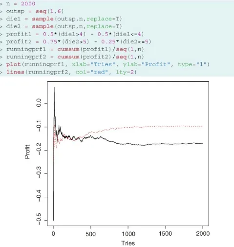
These results tell you two things: (1) both bets lose money in the long term because both have negative expected profits; (2) although both are disadvantageous, the second is better than the first because it is the least negative.
You can verify the results by simulating 2000 repetitions of each of the two bets using code that is very similar to the one we used in Section 2.2 (see Figure 2.2, as well as Sidebar 2.1 for details on how to simulate outcomes from nonequiprobable experiments in R).[
Note that, although early on the profit from the first bet is slightly better than the profit from the second, once you have been playing both bets for a while the cumulative profits revert to being close to the respective expected values.
Consider now the following pair of bets:
Wager 3: You pay $3 to enter and I roll a die. If it comes up 1, 2, or 3, then I keep your money. If it comes up 4, 5, or 6, then I give you back $6 (your original bet plus a $3 profit).
Wager 4: You pay $3 to enter and I roll a die. If it comes up 1 or 2 then I get to keep your money. If it comes up 3, 4, 5, or 6 then I give you back $4 and a half (your original $3 plus a profit of $1 and a half).
The expectations associated with these two bets are
So, both bets are fair, and the expected value does not help us choose among them. However, clearly these bets are not identical. Intuitively, the first one is more “risky”, in the sense that the probability of losing our original bet is larger. We can formalize this idea using the notion of variance of a random variable:
The variance of a random variable X with outcomes is given by
As the formula indicates, the variance measures how far, on average, outcomes are from the expectation. Hence, a larger variance reflects a bet with more extreme outcomes,
which often translates into a larger risk of losing money. For instance, for wagers 3 and 4, we have
more wildly and takes longer than the less variable wager 4 to get close to the expected value of 0.[
Figure 2.3 Running profits from Wagers 3 (continuous line) and 4 (dashed line).
Just like the expectation, the variance has some interesting properties. First, the variance is always a nonnegative number (a variance of zero corresponds to a nonrandom
number). In addition,
If X is a random variable and a and b are two constant (non-random numbers), then
a higher risk of losing money but also the possibility of making more money in a single round of the game (the maximum profit from wager 3 is actually twice the maximum profit from wager 4). Therefore, if you want to make money as fast as possible (rather than play for as long as you can), you would typically prefer to take an additional risk and go for the bet with the highest variance!
2.5 Utility Functions and Rational Choice Theory
The discussion about the comparison of bets presented in the previous section is an
example of the application of rational choice theory. Rational choice theory simply states that individuals make decisions as if attempting to maximize the “happiness” (utility) that they derive from their actions. However, before we decide how to get what we want, we first need to decide what we want. Therefore, the application of the rational choice theory comprises two distinct steps:
1. We need to define a utility function, which is simply a quantification of a person's preferences with respect to certain objects or actions.
2. We need to find the combination of objects/actions that maximizes the (expected) utility.
For example, when we previously compared wagers, our utility function was either the monetary profit generated by the wager (in our first example) or a function of the
variance of the wager (when, as the second example, the expected profit from all wagers was the same). However, finding appropriate utility functions for a given situation can be a difficult task. Here are some examples:
1. All games in a casino are biased against the players, that is, all have a negative expected payoff. If the player's utility function were based only on monetary profit, nobody would gamble! Hence, a utility function that justifies people's gambling should include a term that accounts for the nonmonetary rewards associated with gambling.
2. When your dad used to play cards with you when you were five years old, his goal was probably not to win but to entertain you. Again, a utility function based on money probably makes no sense in this case.
3. The value of a given amount of money may depend on how much money you already have. If you are broke, $10,000 probably represents a lot of money, and you would be unwilling to take a bet that would make you lose that much, even if the expected profit were positive. On the other hand, if you are Warren Buffett or Bill Gates, taking such a bet would not be a problem.
those that have lower variances. For this reason, in this book, we will usually look at the expected value of the game first and, if the expected value happens to be the same for two or more choices, we will expect the player pick the one with the lower variance (which, as we discussed before, minimizes the risk).
2.6 Limitations of Rational Choice Theory
Rational choice theory, although useful to formulate models of human behavior, is not always realistic. A good example of how people will easily deviate from the strict rational behavior as defined above is Ellsberg's Paradox. Assume that you have an urn that
contains 100 blue balls and 200 balls of other colors, some of which are black and some of which are yellow (exactly how many are of each color is unknown). First, you are offered the following two wagers:
Wager 1: You receive $10 if you draw a blue ball and nothing otherwise. Wager 2: You receive $10 if you draw a black ball and nothing otherwise.
Which of the two wagers would you prefer? After answering this question, you are offered the following two wagers,
Wager 3: You receive $10 if you draw a blue or yellow ball and nothing otherwise. Wager 4: You receive $10 if you draw a black or yellow ball and nothing otherwise. No matter how many yellow balls there really are, rational choice theory (based on
calculating expected values for each wager) predicts that if you prefer Wager 2 to Wager 1, then you should also prefer Wager 4 to Wager 3, and vice versa. To see this, note that the
expected payoff from Wager 1 is (because there are exactly 100 blue
balls in the urn). Consequently, for Wager 2 to be preferable to wager 1, you would need to assume that the urn contains more than 100 black balls. But if you assume that there are at least 100 black balls in the urn, the expected value for Wager 3 would be at most
(because there are at most 99 yellow balls and exactly 100 blue ball in the urn), while the expected profit for Wager 4 would always be
, making Wager 4 always better than Wager 3. The paradox arises from the fact that many people who prefer Wager 1 to Wager 2 actually prefer Wager 4 to Wager 3. This might be because people do not know how to react to the uncertainty of how many black and yellow balls there are and prefer the wagers where there is less (apparent) uncertainty.
Another interesting example is Allais paradox. Consider three possible prizes – prize A: $0, prize B: $1,000,000, and prize C: $5,000,000. You are first asked to choose among two lotteries:
Lottery 1: You get prize B ($1,000,000) for sure.
($1,000,000) with probability 0.89, or you get prize C ($5,000,000) with probability 0.10.
Then you are offered a second set of lotteries
Lottery 3: You get prize A (nothing) with probability 0.89, or you get prize B ($1,000,000) with probability 0.11.
Lottery 4: You get prize A (nothing) with probability 0.90, or you get prize C ($5,000,000) with probability 0.10.
Again, many subjects report that they prefer Lottery 1 to Lottery 2 and Lottery 4 to Lottery 3, although rational choice theory predicts that the persons who choose Lottery 1 should choose Lottery 3 too.
The Allais paradox is even subtler than Elsberg's paradox, because each wager (by itself) has an obvious choice (1 and 4, respectively), but taking the two wagers together, if you choose option 1 in the first wager, you should rationally choose option 3 in the second wager because they are essentially the same option. The way we make sense of this (talk about a paradox!) is by noticing that Lottery 1 can be seen as 89% of the time winning $1 million and the remaining 11% winning $1 million. We look at Lottery 1 in this unusual way because it will be easier to compare it to Lottery 3 (where we win nothing 89% of the time and $1 million 11% of the time). We can change the way we look at Lottery 4 for the same reason (to better compare it to Lottery 2): we win nothing 89% of the time, nothing another 1% of the time, and $5 million 10% of the remaining time. Table 2.1 summaries this alternative description for the lotteries.
Table 2.1 Winnings for the different lotteries in Allais paradox
Lottery 1 Lottery 2 Lottery 3 Lottery 4
Wins $1 million 89%
of the time Wins $1 million 89%of the time Wins nothing 89% ofthe time Wins nothing 89% ofthe time Wins $1 million 11%
of the time Wins nothing 1% ofthe time Wins $1 million 11%of the time Wins nothing 1% ofthe time Wins $5 million 10%
of the time Wins $5 million 10%of the time
You can see that Lotteries 1 and 2 are equivalent 89% of the time (they both give you $1 million) and that Lotteries 3 and 4 are the same also 89% of the time (they give you
nothing). Let's look at the table if we cross out the row corresponding to what is supposed to happen 89% of the time.
Table 2.2 Winnings for 11% of the time for the different lotteries in Allais paradox
Lottery 1 Lottery 2 Lottery 3 Lottery 4
Wins $1 million 11%
Wins $5 million 10%
of the time Wins $5 million 10%of the time
In Table 2.2, we see very clearly that Lotteries 1 and 3 are the same choice and that
Lotteries 2 and 4 are the same choice too. Hence, the conclusion from this paradox is that by adding winning $1 million 89% of the time in the first wager compared to the second wager, people deviate from the rational choice across wagers even though there's no reason to do so.
The bottom line from these two paradoxes is that, although rational choice is a useful theory that can produce interesting insights, some care needs to be exercised when applying those insights to real life problems, because it seems that people will not necessarily make “rational” choices.
2.7 Exercises
1. Use the definition of rational choice theory to discuss in which sense gambling can be considered “rational” or “irrational.”
2. Using the basic principles of the “rational player” described in the text (mainly that a player will always try to maximize its expected value and secondly minimize the variance of the gains), decide which of wagers below would the player choose. In all the wagers, the player is required to pay $1 to enter the wager.
Wager 1: When you flip a coin and heads comes out, you lose your dollar. If tails comes out, you get your dollar back and get an additional $0.25.
Wager 2: When you roll a die and 1 or 2 comes out, you lose your dollar; if a 3 or a 4 comes out, you get your dollar back; and if a 5 or a 5 comes out, you get your dollar back and an additional $0.50.
Wager 3: If you roll a die and 1, 2, or 3 comes out, you lose your dollar. If a 4 comes out, you receive your dollar back, and if a 5 or a 6 comes out, you receive your
dollar back and an additional $0.50.
3. The values of random variables are characterized by their random variability.
Explain in your own words what aspect of that variability is the expected value trying to capture. What aspect of the random variability is the variance trying to capture?
4. If you are comparing the variance of two different random variables and you find out one is much higher than the other, what does that mean?
5. Does high variability in the profit of a wager mean higher risk or lower risk of losses?
7. Comment on the following statement: “A rational player will always choose a wager with high variability because it allows for higher gains.”
8. Consider the three different stocks and their profits. Which one would a rational player choose?
Stock A: This stock will give you a net profit of $100 with a probability 0.8, a net profit of $150 with probability 10%, a net profit of $200 with probability 5% or net profit of $500 with probability 5%.
Stock B: This stock will give you a net profit of $65 with a probability 0.8, a net profit of $15 with probability 10%, a net profit of $40 with probability 5% or net profit of $50 with probability 5%.
Stock C: This other stock will give you a net profit of $100 with a probability 0.5, a net profit of $150 with probability 20%, a net profit of $200 with probability 15% or net profit of $500 with probability 15%.
9. Rank your preferences for the following four lotteries (all cost $1 to enter). Explain your choices:
L1: Pays 0 with probability 1/2 and $40,000 with probability 1/2. L2: Pays 0 with probability 1/5 and $25,000 with probability 4/5.
L3: Pays $10,000 (so you need to pay $10,000 if you lose!!) with probability 1/2 and $50,000 with probability 1/2.
L4: Pays $10 with probability 1/3 and $30,000 with probability 2/3.
10. Let's say you finally got some money to buy a decent car. You have two
alternatives: alternative corresponds to buying a 10-old Corolla and alternative corresponds to buying a brand new Corolla. Each alternative has different types of costs involved (the initial cost of the car and future maintenance costs).
For option , there is a 80% probability that on top of the cost of $10,000 to buy the car we will have a $2000 cost for major work on the car in the future. There is also a probability of 15% for the future costs to be as high as $3000 (for a total cost of $13,000). Finally, the more unlucky are subject to the probability of 5% that future costs be as high as $5000 (for a total cost of $15,000).
For option , there's a pretty high probability (90%) that there are no major costs in maintaining the car in the future and you are subject to just the cost of buying the car ($20,000). There is some chance (say 5%), though, that you might need a new transmission or other major work (say, involving $1000 in costs). There's a smaller probability (3%) of some more serious work being necessary (say
something around $2000). And, for the really unlucky, a 2% chance one might need some serious work done (costing something like $3000).
11. An urn contains 30 yellow balls and 70 balls of other colors (which can be either red or blue). Suppose you are offered the following two bets:
Wager 1: You receive $10 if you draw a yellow ball. Wager 2: You receive $10 if you draw a blue ball.
If you prefer the second bet over the first, which one of the following two wagers would you prefer if you are a rational player?
Wager 3: You receive $20 if you draw a red ball.
Wager 4: You receive $15 if you draw a yellow or blue ball.
12. [R] Simulate the profit of both pairs of wagers in the previous exercise and plot the results to see if you made the right decision.
13. A certain health condition has two possible treatments
Treatment A, if successful, will extend the lifetime of the patient by 36 months. If it fails, it will neither increase nor reduce the expected lifetime of the patient. Clinical trials show that 20% of patients respond to this treatment.
Treatment B, if successful, will increase the lifetime of the patient by 14 months, and 65% of the patients respond to it. In addition, 10% of the patients subject to this treatment suffer from an adverse reaction that reduces their expected lifetime by 2 months, and for the rest (25%) the treatment has no effect.
Chapter 3
Roulette
Roulette is one of the simpler games available in modern casinos and has captured the popular imagination like no other. In fact, the game has been featured in countless movies such as Humphrey Bogart's 1942 Casablanca, Robert Redford's 1993 Indecent Proposal, and the 1994 German movie Run, Lola, Run.
3.1 Rules and Bets
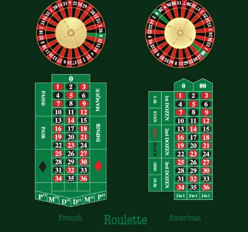
Roulette is played using a revolving wheel that has been divided into numbered and color-coded pockets. There are 38 pockets in the American roulette (popular in the United
States), or 37 pockets in the European roulette (common in Monte Carlo and other
Figure 3.1 The wheel in the French/European (left) and American (right) roulette and respective areas of the roulette table where bets are placed.
Bets in roulette are placed by moving chips into appropriate locations in the table.
Roulette bets are typically divided into inside and outside bets. Outside bets derive their name from the fact that the boxes where the bets are placed surround the numbered boxes.
The simplest inside bet is called a straight-up, which corresponds to a bet made to a
specific number. To place this bet, you simply move your chips to the center of the square marked with the corresponding number. The payoff odds from a straight-up bet are 35 to 1, which means that if your number comes up in the wheel, you get your original bet back and get a profit of $35 for each dollar you bet. Other inside bets, such as the split or the street, are described in Table 3.1.
color as the one you picked. Similarly, you win an even bet if the number that comes up in the roulette is a nonzero even number. In both cases, the payoff odds are 1 to 1, so they are often called even bets. However, as we will see below, these even bets are not fair bets because the winning odds are not 1 to 1. A list of outside bets is presented in Table 3.2. This list corresponds to the bets and payoffs most commonly used in the United States; some casinos allow for additional bets, or might slightly change the payouts associated with them.
Table 3.1 Inside bets for the American wheel
Bet
name You are betting on… Placement of chips Payout
Straight-up A single number between 1 and 36 In the middle of number square 35 to 1
Zero 0 In the middle of the 0 square 35 to 1
Double
zero 00 In the middle of the 00 square 35 to 1
Split Two adjoining numbers
(horizontally or vertically) On the edge shared by bothnumbers 17 to 1
Street Three numbers on the same
horizontal line Right edge of the line 11 to 1
Square Four numbers in a square layout
(e.g., 19, 20, 22, and 23) Corner shared by all four numbers 8 to 1
Double
street Two adjoining streets (see Streetrow) Rightmost on the line separatingthe two streets 5 to 1 Basket One of three possibilities: 0, 1, 2 or
0, 00, 2 or 00, 2, 3 Intersection of the three numbers 11 to 1
Top line 0, 00, 1, 2, 3 Either at the corner of 0 and 1 or
the corner of 00 and 3 6 to 1
From a mathematical perspective, the game of roulette is one of the simplest to analyze. For example, in American roulette, there are 38 possible outcomes (the numbers 1–36 plus 0 and 00), which are assumed to be equiprobable. Hence, the probability of any number coming up is 1/38. This means that the expected profit from betting $1 on a straight-up wager is
casinos remain a predictably profitable business (remember the law of large numbers for expectation from Chapter 2).
Take now an even bet. There are 18 nonzero even numbers; therefore, the expected profit from this bet is
Table 3.2 Outside bets for the American wheel
Bet name You are betting on… Placement of chips Payout
Red/black Which color the roulette will show Box labeled Red 1 to 1
Even/odd Whether the roulette shows a nonzero even
or odd number Boxes labeled Even orOdd 1 to 1
1–18 Low 18 numbers Box labeled 1–18 1 to 1
19–36 High 18 numbers Box labeled 19–36 1 to 1
Dozen Either the numbers 1–12 (first dozen), 13–24
(second dozen), or 25–36 (third dozen) First 12 boxes (firstdozen), second 12 boxes (second dozen), third 12
This same calculation applies to odd, red, black, 1–18 and 19–36 bets. On the other hand, for a split bet, we have
and for a street bet
As a matter of fact, the house advantage for almost every bet in American roulette is the same ( ). Among the bets discussed in Tables 3.1 and 3.2, the only exception is the top line bet, which is more disadvantageous than the other common bets:
each of the numbers included in it using straight-up bets! To see this, consider betting $5 on a top line bet versus betting $1 simultaneously on each of the numbers in the top line bet (0, 00, 1, 2, 3). Due to the properties of expectations (recall Chapter 2), the expected profit from the first wager is
while, the expected profit from the second bet is
This means that with the top line bet you lose on an average 50% more even though you are betting the same amount of money to exactly the same numbers!
Although most bets in roulette are equivalent in terms of their expected value, the risk associated with them differs greatly. Take, for example, the straight-up bet:
while the variance of a color bet is
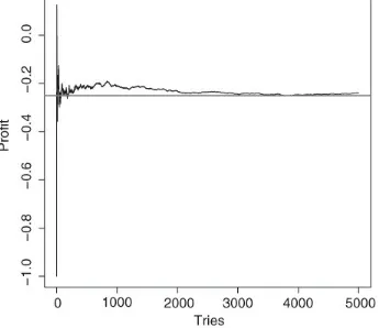
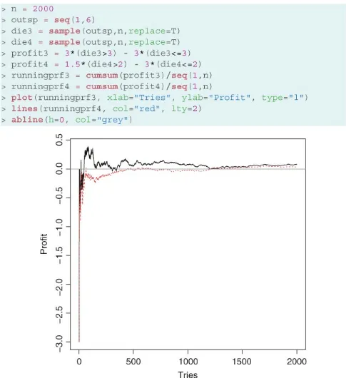
Figure 3.2 Running profits from a color (solid line) and straight-up (dashed line) bet.
Figure 3.2, which shows the results from these simulations, is consistent with the
discussion we had before: although the average profits from both bets eventually tends to converge toward the expected value of , the straight-up bet (which has the highest variance) has much more volatile returns.