Chp02 – Discrete Random Variables

Introduction to Probability

SECOND EDITION

Dimitri

P.

Bertsekas and John N. Tsitsiklis

Massachusetts Institute of Technology

WWW site for book information and orders

http://www.athenasc.com

2

Discre te R andom Variables

Contents

2. 1 . Basic Concepts . . . .

2.2. Probability Mass Functions

2.3. Functions of Random Variables

2.4. Expectation, Mean, and Variance

2.5. Joint PMFs of Multiple Random Variables

2.6. Conditioning . . . .

.

.

2.7. Independence . . . .

2.8. Summary and Discussion

Problems . . . .

p. 72

p. 74

p. 80

p. 81

p. 92

p. 97

. p. 109

. . p. 1 1 5

. p . 1 19

1

nlany probabilist ic outcomes are instrunlent readings

or stock prices.

are not

.

but

2

corre-IS st froIn a given

populat ion. we may wish to consider t heir grade point average. When it is useful to

is done through t he notion of a

variable,

the focus of the present

an and t he possible

(

the

salnpie space) 1 a randoIn variable associates a particular nunlber with each

out-conle: see Fig.

1 .

\iVe t o this as the

the t l\Iathelnatically� a

2 . 1 : V isualizat ion of a random vari able . It is a fu nct ion that a numerical value to _{each poss i ble} o_{ut c}o_me of _{the experi ment . ( b) A n} of a random variahle. The consists o f two rolls o f a 4-sided

t h e random variable _{is t he max i mum} of _{t he} two rol ls . _{I f} t_he outcome of _the

is (4. 2) . is 4.

are sonle of variables:

(a) an i nvolving a sequence of 5 tosses

he_ads t he sequence is a randon)

a t_{he nunlber of}

Sec. 2. 1 Basic Concepts

73

of heads and tails is not considered a random variable because it does not

have an explicit numerical value.

(

b

)

In an experiment involving two rolls of a die. the following are examples of

random variables:

(

i

)

The sum of the two rolls.

(

ii

)

The number of sixes in the two rolls.

(

iii

)

The second roll raised to the fifth power.

(

c

)

In an experiment involving the transmission of a message, the time needed

to transmit the message. the number of symbols received in error. and the

delay with which the message is received are all random variables.

There are several basic concepts associated with random variables. which

are summarized below. These concepts will be discussed in detail in the present

chapter.

Main Concepts Related to Random Variables

Starting with a probabilistic model of an experiment :

•

A

random variable

is a real-valued function of the outcome of the

experiment.

•

A

function of a random variable

defines another random variable.

•

We can associate with each random variable certain ';averages" of in­

terest, such as the

mean

and the

variance.

•

A random variable can be

conditioned

on an event or on another

random variable.

•

There is a notion of

independence

of a random variable from an

event or from another random variable.

A random variable is called

discrete

if its range

(

the set of values that it

can take

)

is either finite or count ably infinite. For example. the random variables

mentioned in

(

a

)

and

(

b

)

above can take at most a finite number of numerical

values, and are therefore discrete.

A random variable that can take an uncountably infinite number of values

is not discrete. For an example. consider the experiment of choosing a point

a from the interval

[- 1. 1] .

The random variable that associates the numerical

value a2 to the outcome a is not discrete. On the other hand. the random variable

that associates with a the numerical value

{ I.

if a > O.

sgn

(

a

) =

O. if a

=

O�

74 Discrete Random Variables Chap. 2

is discrete.

In thi� chapter. we focus exclusively on discrete random variables, even

though ''''e will typically omit the qualifier '-discrete."

Concepts Related to Discrete Random Variables

Starting with a probabilistic model of an experiment:

•

A

discrete random variable

is a real-valued function of the outcome

of the experiment that can take a finite or count ably infinite number

of values.

•

A discrete random variable has an associated

probability mass func­

tion

(PMF

)

l

which gives the probability of each numerical value that

the random variable can take.

•

A

function of a discrete random variable

defines another discrete

random variable, whose PlVIF can be obtained from the PMF of the

original random variable.

We will discuss each of the above concepts and the associated methodology

in the following sections. In addition. we will provide examples of some important

and frequently encountered random variables. In Chapter 3, we will discuss

general (not necessarily discrete) random variables.

Even though this chapter may appear to be covering a lot of new ground,

this is not really the case. The general line of development is to simply take

the concepts from Chapter

1

(probabilities, conditioning, independence, etc.)

and apply them to random variables rather than events, together with some

convenient new notation. The only genuinely new concepts relate to means and

variances.

2.2

PROBABILITY MASS FUNCTIONS

The most important way to characterize a random variable is through the prob­

abilities of the values that it can take. For a discrete random variable

X,

these

are captured by the

probability mass function

(PMF for short) of

X,

denoted

px .

In particular. if

x

is allY possible value of

X .

the

probability mass

of

x.

denoted

px (x).

is the probability of the event

{X = x}

consisting of all outcomes

that give rise to a value of

X

equal to

x:

px (r) = P ({X x}) .

Sec. 2.2 Probability Mass Functions

In what follows, we will often omit the braces from the event/set notation

when no ambiguity can arise. In particular, we will usually write

P(X

= x

)

in

place of the more correct notation

P ({ X

= x

}

)

,

and we will write

P (X

E

S)

for the probability that

X

takes a value within a set

S.

We will also adhere

to the following convention throughout:

we will use upper case characters

to denote random variables, and lower case characters to denote real

numbers such as the numerical values of a random variable.

Note that

x

where in the summation above,

x

ranges over all the possible numerical values of

X.

This follows from the additivity and normalization axioms: as

x

ranges over

all possible values of

X,

the events

{X

=

x}

are disjoint and form a partition of

the sample space. By a similar argument, for any set

S

of possible values of

X,

we have

P(X

E

S)

=

L px(x).

xES

For example, if

X

is the number of heads obtained in two independent tosses of

a fair coin, as above, the probability of at least one head is

2

1

1

3

P (X

>

0)

=

L Px(x)

= 2

+

4

₌

4·

x=l

Calculating the PMF of

X

is conceptually straightforward, and is illus­

trated in Fig. 2.2.

Calculation of

the PMF

of a Random Variable

X

For each possible value

x

of

X:

1 .

Collect all the possible outcomes that give rise to the event

{X

=

x}.

2. Add their probabilities to obtain

px(x).

The Bernoulli Random Variable

5 16 3

.r

2 . 2 : I l l ustration of the method to _calculate the PMF of _{a r}a_ndo m

variable X. For each the outcomes that rise to X = x and add th_eir to obtain _{Px Calcu l at ion of} the

P !'d F Px of _{the random} variable X max imum _roll i_n two _rolls

of a fair 4-sided die . There are four values X , 1 , 2. 3, 4. To

calculate p x x I we add the of the outcomes that

there are three outcomes that r ise _{to x = 2}

.2). 1 ) . Each of these outcomes has 1 so PX

as indicated in t h e

- r·

IS

as:

if a if _a

or a

if k = 1 . if k

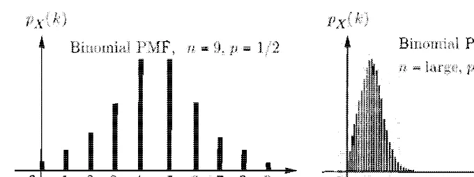
2.2

a

n k

2 . 3 : The P �l F of a binom ial ran dom variable . If _{p = 1/2 ,} the P I\lF is

around n/2. the P i\ I F _{is skewed towards 0 if P < 1/2 . and}

77

towards n i f p > 1/2.

( a) state a t_el_ephone at a given tinle t hat can be her or busy.

(b) A person who can be eit her healt hy or sick with a certain disease.

( c) The _{preference of} a person who can be either for or against a litical

var iables, one can con

-as the binonlial variable,

A coin is tossed n t i nles. the coi n conles up a head with probability

p, and a tail of Let X be the

of heads i n

consists of the binonlial

= k) =

(nk)

k

=

0, 1 ,

. .. � n .

(Note that we sinlplify notation use X ,

to denote t he values of integer-valued random vari ables . ) The nornlalization

property, is as

cases of binonlial are Fig. 2.3.

we and toss a coi n with probability

1 2 3 k

2.4: The

random variable. It decreases as a with

1 -p.

number by

(1 -

p) k -1

P

is

tails followed a

00

L

(k)

=

k= l

px (k) =

( 1 -

p)k-00

( 1 - = p

k= l

to come up for

00

k=O

k = 1 , • • • j

1

I - p)k = P " l _

I - p)

= 1 .

example, it could mean passing a test in a given finding a missing

given

A Poisson random variable has a PNIF by

In _a

px (k) = Ak k =

0, 1 , 2, . . . ,

2

IS

the see 2 . 5 . _{This is a}

80 Discrete Random Variables Chap. 2

2.3

FUNCTIONS OF RANDOM VARIABLES

Given a random variable

X,

one may generate other random variables by ap­

plying various transformations on

X.

As an example, let the random variable

X

be today's temperature in degrees Celsius, and consider the transformation

Y

=

1.8X

+

32. which gives the temperature in degrees Fahrenheit . In this

For example. i f we wish to display temperatures on a logarithmic scale, we would

want to use the function

g(

X )

=

log

X.

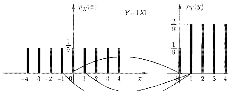
Y = I XI

-4 - .] _y

Figure 2 . 6 : The P�IFs of X and Y = I X I in Example 2. 1 .

another related exanlple . let Z =

X2 .

To obtain the P�1F of we it as t he square the or as square of

Y =

I I.

=

L

_{{ x I}

(x)

or

the formula pz (z) = _{{ Y I = z }}

py (y).

we obtain

The

pz (z) =

{

1 if z = o.

2/9. if z = 1 . 4 . 9. 1 6 .

o f

a

randoln variable of all

O. ot herwise.

provide� u� ,vith �everal ntllubert).

X .

It

is .

to

pro

ba-IHllnber. is by the

(in p

ro

p

ortion to

probabilities) average

motivation. suppose yon a of lllany

spin . one nurnbers Tn l . m'2 . . . 11 1 n cornes up w'ith corresponding proba

-. P2 ,

. . . . that \Vh at is

the am_ount _to

and are a

Suppo:se t hat _{you �pi n}

t

that the o utcolne is m j . t he total alllo unt received is m 1 kl

+

arnount spin is

If the nUlnber of spins k is

bilit ies as frequencies. it is

if we are willing to

82 Discrete Random Variables

fraction of times that is roughly equal to

Pi:

ki

_{"" P'}

k

""

t ,

i

=

1 ,

.. ., no

Thus, the amount of money per spin that you "expect" to receive is

Motivated by this example, we introduce the following definition.

t

Expectation

Chap. 2

We define the

expected value

(

also called the

expectation

o

r

the

mean)

of a random variable

X,

with PMF

P x,

by

E[X]

=

L xPx(x).

x

Example 2.2. Consider two independent coin tosses, each with a

3/4

probability of a head, and let X be the number of heads obtained. This is a binomial random variable with parameters

n =

2

and

p

=

3/4.

Its PMF is

so the mean is

{

(1/4)2 ,

if k

=

0,

px (k)

=

2 · (1/4) . (3/4),

if

k

=

1,

(3/4)2 ,

if k

=

2,

( 1 ) 2 ( 1 3 ) ( 3 ) 2 24 3

E[X] = o ·

4

+

1 · 2 ·

4 . 4

+

2 ·

4

=

16

=

2'

t When dealing with random variables that take a countably infinite number of values, one has to deal with the possibility that the infinite sum

Lx

xpx (x)

is not well-defined. More concretely, we will say that the expectation is well-defined if

Lx

Ixlpx (x)

< 00. In this case, it is known that the infinite sum

Lx

xpx (x)

converges

to a finite value that

is

independent of the order in which the various terms are summed. For an example where the expectation is not well-defined, consider a random variable X that takes the value

2k

with probability

2-k,

for k =

1,2,

. . . . For a more subtle example, consider a random variable X that takes the values

2k

and

_2k

with probability

2-k,

for k =

2,3,

. . . . The expectation is again undefined, even though the

Expecta tion,

It useful to view the mean of X as a "representative" value of X, which

its more

by viewing the mean as

explained in

Fig.

2.7. In particular, if

that point must to mean.

the PMF,

sense

around a

2.1: of the mean as a center of a bar with

a weight p X placed at each point x with p X > 0, the center of

the point at whi ch the sum of the torques from the weights to its left is to the sum of the from the to its right:

L(X

-c)px (x) = O.

the center of gravity is equal to t he mean E[X] .

Besides the mean, there are several its

_PMF.

as

E[xn] ,

the

terminology, the moment of

mean.

j ust the

The most important quantity associated a variable X j other

than IS IS

the expected of the

(X - ) 2 can only

by

var(X) as

(X -

)2,

- E[X] ) 2

]

.

is

its mean. is defined

84 Discrete Random Variables Chap. 2

The standard deviation is often easier to interpret because it has the same units

as X. For example, if X measures length in meters, the units of variance are

square meters, while the units of the standard deviation are meters.

One way to calculate var(X), is to use the definition of expected value,

after calculating the

PMF

_{of the random variable (X}

-

E

[

Xl) 2 . This latter

random variable is a function of X, and its

PMF

can be obtained in the manner

discussed in the preceding section.

X

around 0, and can also be verified from the definition: 1

4

It turns out that there is an easier method to calculate var(X), which uses

the

PMF

of X but

does not require the

PMF

of

(X - E[Xl) 2. This method

is based on the following rule.

Expected Value Rule for Functions of Random Variables

Let X be a random variable with

PM

F

px,

and let

g(X)

be a function of

X. Then, the expected value of the random variable

g(

X) is given by

E[g(X)]

=

Lg(x)px(x).

x

To verify this rule, we let

Y

=

g(X) and use the formula

py(y)

=

px(x)

Sec. 2.4 Expectation, l\:Iean, and Variance

derived in the preceding section. We have

E[g(X)]

=

E[Y]

=

L YPY(Y)

y

=

_{L Y L px(x)}

y { x I g (x)=y}

=

L L ypx(x)

y {x l g (x)=y }

=

L L g(x)px(x)

y {x I g(x } =y}

=

Lg(x)px(x).

x

Using the expected value rule, we can write the variance of

X

as

var(X)

=

E [(X - E[X])2]

=

L(x - E[X])2pX(x).

x

Similarly, the nth moment is given by

x

and there is no need to calculate the P:l\fF of

X

n .

Example 2.3 (continued) . For the random variable X with PMF

we have

( ) {I

/9. if

x

is an integer in the range [-4. 4J . px

x = O.

otherwise,

var(X)

=

E

[

(

X - E[xJ

)

2]

=

L(x

-E[XJ

)

2pX (X) x

(since E[XJ = 0)

1

=

'9

( 16 + 9 + 4 + 1 + 0 + 1 + 4 + 9 + 16) 60

g'

which is consistent with the result obtained earlier.

86 Discrete Random Variables Chap. 2

As we have already noted, the variance is always nonnegative, but could it

be zero? Since every term in the formula

Lx(X - E[X])2pX(x)

for the variance

is nonnegative, the sum is zero if and only if

(x - E[X])2px(x)

₌

°

for every

x.

This condition implies that for any

x

with

px(x)

>

0, we must have

x

₌

E[X]

and the random variable

X

is not really "random" : its value is equal to the mean

E[X],

with probability

_{1 .}

Variance

The variance var

(

X

)

of a random variable X is defined by

var

(

X

)

=

E

[

(

X

- E[X])2

]

,

and can be calculated

as

x

It is always nonnegative. Its square root is denoted by

a

x

and is called the

standard deviation.

Properties of Mean and Variance

\Ve will now use the expected value rule in order to derive some important

properties of the mean and the variance. We start with a random variable

X

and define a new random variable Y, of the form

Y

=

aX + b,

where

a

and

b

are given scalars. Let us derive the mean and the variance of the

linear function Y. We have

E[Y]

=

L(ax + b)px(x)

=

a LXPX(x) + b LPx(x)

=

aE[X] + b.

x

x

x

Furthermore,

var

(

Y

)

=

L(ax + b - E[aX + b])2pX(x)

x

x

x

Sec. 2.4 _{Expectation, Mean, and Variance}

Mean and Variance of a Linear Function of a Random Variable

Let

X

be a random variable and let

Y

=

aX

+ b.

where

a

and

b

are given scalars. Thenl

E(Y]

=

aE(X]

+ b,

var

{

Y

)

=

a2

var

(

X

)

.

87

Let us also give a convenient alternative formula for the variance of a

random variable

X.

Variance in Terms of Moments Expression

var

(

X

)

=

E[X2J - (E[X])2.

This expression is verified

as

follows:

var

(

X

)

=

L(x - E[X])2pX(x)

x

=

L (X2 2xE[X]

+

(E[X])2)px(.T)

x

x x

=

E[X2] 2(E[X])2

+

(E[X])2

=

E[X2] (E[X])2.

x

We finally illustrate

by

example a common pitfall: unless

g(X)

is a linear

function, it is not generally true that

E [g(X)]

is equal to

g(E[X]).

Example

(

2.4. Average Speed Versus Average Time. If the weather is good which happens with probability 0.6) . Alice walks the 2 miles to class at a speed of V

=

5

miles per hour, and otherwise rides her motorcycle at a speed of V = 30

miles per hour. What is the mean of the time T to get to class?

A correct way to solve the problem is to first derive the PMF of T.

() {

0.6. if t

=

2/5 hours.

PT

t

= _.

0.4. If t = 2/30 hours.

and then calculate its mean by

2 2 4

E

[

T

]

= 0.6 .

5"

+ 0.4 .

88 Discrete Random Variables

However, it is wrong to calculate the mean of the speed V, E

[

V

] = 0.6 · 5

+

0.4 · 30

=

15

miles per hour, and then claim that the mean of the time

T

is

2 2

E

[

V

] = 15

hours.

To summarize, in this example we have

2

T =

_{V '}

Chap. 2

Mean and Variance of Some Common Random Variables

We will now derive formulas for the mean and the variance of a few important

random variables. These formulas will be used repeatedly in a variety of contexts

throughout the text .

Example 2.5. Mean and Variance of the Bernoulli. Consider the experi­ ment of tossing a coin, which comes up a head with probability p and a tail with probability

1 -

p. and the Bernoulli random variable X with PMF

px (k)

=

{ P,

₁

�

f k

= 1.

-p. If k

= O.

The mean. second moment. and variance of X are given by the following calcula-tions:

E[X]

= 1

. p +

0 . (1

-p)

=

p.

E[X2] = 12 .

_P

+

0 . (1

-p)

=

p,

var(X)

=

E[X2] -

(

E

[

X

]) 2 =

_P

_

p2 = p(1

_

p) .

Example 2.6. Discrete Uniform Random Variable. What is the mean and variance associated with a roll of a fair six-sided die? If we view the result of the roll as a random variable X, its PMF is

px (k)

=

{

1/6,

_0,

if k _otherWise.

= �. 2,3,4,5,6,

Since the PMF is symmetric around

3.5.

we conclude that

E[X] = 3.5.

Regarding the variance, we have

var(X)

=

E

[

X

2]

_

(

E

[

X

]) 2

2.4

1

• • •

2 . 8 : P IvlF _{of the discrete random variable that is uniformly}

dis-tributed between two a and b. Its mean and variance are

E[X]

_

a + b var( X ) = ( b - a ) ( b - a + 2)

12

which yields var(

X

)

= 35/ 1 2.

89

takes one out of a range of contiguous integer values � with equal probability. i\lore a random variable a P?v!F of t he

px

(k)

=

{

b -

+

1 .

O.

if k = a . a + 1 . . . , . b.

otherwise. a

b

are two a < b: see The mean is

a + b

2

as can be seen inspection , is ( a + b) /2 .

calculate the variance of

X .

we first consider the simpler case w here a = 1 and

b =

n.

It can on

n

1

n

1

=

G (n +

1 )

+

1 ) .

k = l

) =

1 1 2

=

6" (n +

1) ( 2n + 1) -

4'

(11,

+

1 )

1

= ₊

1)

_{+ 2 -} - 3)

90 Discrete Random Variables Chap. 2

For the case of general integers a and b, we note that a random variable which is uniformly distributed over the interval [a

,

b] has the same variance as one which

The last equality is obtained by noting that

is the normalization property for the Poisson PMF.

A similar calculation shows that the variance of a Poisson random variable is also A: see Example 2.20 in Section 2.7. We will derive this fact in a number of different ways in later chapters.

Decision Making Using Expected Values

Expected values often provide a convenient vehicle for optimizing the choice

between several candidate decisions that result in random rewards. If we view

the expected reward of a decision

as

its "average payoff over a large number of

2. 4

as

first question attempted is answered incorrectiy, the quiz terminates, i.e. , the person is not allowed to attempt the second If first question is answered

received?

The answer is not obvious because there is a tradeoff: attempting first the

more but 2

as a random variable X 1 and calcu late

possible 2,9) :

$ 100

$

value E(X] under the two

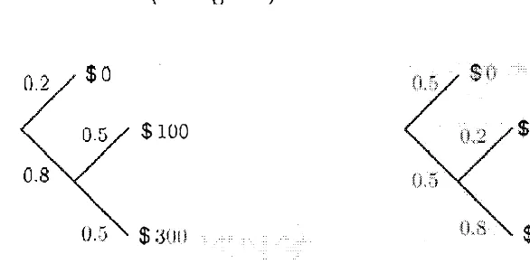
2 . 9 : _{Sequential description of the sample space of the quiz problem}

for the two cases w here we answer q uestion 1 or question 2 first .

(a)

px (0) =

and we have

1

px ( 1 00) = · 0.5,

is (cf.

PX

(300) = 0.8 . 0.5,

E[X]

= 0.8 · 0.5 · 1 00 + 0.8 · 0.5 · 300 = $ 1 60.

(b) Answer question

2

first:

Then the PMF of X is (cf. the right side Fig. 2.9)

px (0) = _px (200) = 0.5 . px (300) = 0.5 · 0.8,

and we

92 Discrete Random Variables Chap. 2

Thus, it is preferable to attempt the easier question

1

first.

Let us now generalize the analysis. Denote by PI and P2 the probabilities of correctly answering questions

1

_{and 2, respectively, and by VI and V2 the corre­} sponding prizes. If question

1

is answered first, we have

while if question 2 is answered first, we have

It is thus optimal to answer question

1

first if and only if

or equivalently, if

PI VI > P2V2

1

-

PI

-

1

_-

_{P2 '}

Therefore, it is optimal to order the questions in decreasing value of the expression pV/(l - p) . which provides a convenient index of quality for a question with prob­ ability of correct answer P and value v. Interestingly, this rule generalizes to the

case of more than two questions (see the end-of-chapter problems) .

2.5

JOINT PMFS OF MULTIPLE RANDOM VARIABLES

Probabilistic models often involve several random variables. For example, in

a medical diagnosis context, the results of several tests may be significant, or

in a networking context . the workloads of several routers may be of interest.

All of these random variables are associated with the same experiment, sample

space, and probability law, and their values may relate in interesting ways. This

motivates us to consider probabilities of events involving simultaneously several

random variables. In this section, we will extend the concepts of PMF and

expectation developed so far to multiple random variables. Later on, we will

also develop notions of conditioning and independence that closely parallel the

ideas discussed in Chapter

1.

Consider two discrete random variables

X

and Y associated with the same

experiment . The probabilities of the values that

X

and Y can take are captured

by the

joint PMF

of

X

and Y, denoted

PX,y.

In particular. if

(x, y)

is a pair

of possible values of

X

and Y, the probability mass of

(x. y)

is the probability

of the event

{X

=

x.

Y

=

y}:

PX.y(x. y)

=

P

(

X

=

x.

Y

=

y).

Sec. 2.5 Joint PMFs of Multiple Random Variables 93

The joint PMF determines the probability of any event that can be specified

in terms of the random variables

X

and Y. For example if

A

is the set of all

pairs

(x,

y)

that have a certain property, then

P((X.

Y) E

A) =

L PX,y(x,

y).

(x.Y)EA

In fact , we can calculate the PMFs of

X

and Y by using the formulas

pX(x)

=

LPx,Y(x,

y),

py (y)

=

LPX,y(x,

y).

Y x

The formula for

P x

(x)

can be verified using the calculation

pX(x) = P(X = x)

=

_L

P(X = x. Y = y)

Y

where the second equality follows by noting that the event

{X =

x}

is the union

of the disjoint events

{X = x.

Y

=

_y

}

as

y

ranges over all the different values of

Y. The formula for

py (y)

is verified similarly. We sometimes refer to

P x

and

py

as the

marginal

PMFs, to distinguish them from the joint PI\IF.

We can calculate the marginal PMFs from the joint PMF by using the

tabular method.

Here. the joint PMF of

X

and Y is arranged in a two­

dimensional table, and

the marginal

PMF

of X or

Y

at a given value 'is obtained

by adding the table entries along a corresponding column or

row,

respectively.

This method is illustrated by the following example and Fig.

2. 10.

Example

2.9. Consider two random variables.

X

and Y, described by the joint PMF shown in Fig. 2. 10. The marginal P�lFs are calculated by adding the table entries along the columns (for the marginal PMF of

X)

and along the rows (for the marginal PMF of V), as indicated.

Functions of Multiple Random Variables

When there are multiple random variables of interest , it is possible to generate

new random variables by considering functions involving several of these random

variables. In particular, a function

Z

= g(X.

Y) of the random variables

X

and

Y defines another random variable. Its PMF can be calculated from the joint

PMF

Px.y

according to

pz(z) =

PX.y

(x, y).

.:1

3

2

1

method for calculating the

PMFs from the P MF i n 2.9. The joint P M F i s

ta ble, where t he number in each square y) gives the value of p x ,

y

y) . To

c alc ulate the marginal PTvI F PX (x) for a given val ue of x , we add the numbers i n

the colu m n t o x . For _Px (2) = Similarly, to calcu late

the P?\1F py (y) for a value of y , we add t he numbers in the row to y . For py (2) = 7/20.

2

Furthermore. the expected value rule for functions and takes the form

[g(X,

x _y

very to

In the special case "iNhere 9 is we

y)pX,y (x, y).

case a

and of

E[aX bY

+

c]

=

aE[X]

+

bE[Y] c.

a

form

aX +bY +c,

Example (continued) .

j oint PMF is given i n Fig. 2.

the random X and Y whose and a new random variab l e Z defi ned

by

z =

X

+ 2Y.

Z can

pz(z) =

PX,y (x, y),

Sec. 2.5 Joint PMFs of Multiple Random Variables

Alternatively, we can obtain E[Z] using the formula

E

[

Z] = E

[

X] + 2E

[

Y] .

PMFs are analogously obtained by equations such

as

and

PX,y (x, y)

=

L PX,y,z(x, y,

z

)

_,

z

96 Discrete Random Variables Chap. 2

The expected value rule for functions is given by

E[g(X,

Y.

Z)]

=

L L L 9(x,

y,

z)pX,Y,z(x,

y,

z),

x _y z

and if

9

is linear and has the form

aX

+

bY

+

cZ

+

d,

then

E[aX

+

bY

+

cZ

+

d]

=

aE[X]

+

bErYl

+

cE[Z]

+

d.

Furthermore, there are obvious generalizations of the above to more than three

random variables. For example, for any random variables

Xl, X2, . . . ,Xn

and

any scalars

a

I ,

a2 .. . . , an,

we have

Example 2. 10. Mean of the Binomial. Your probability class has 300 students and each student has probability 1/3 of getting an A, independent of any other independent trials, it is a binomial random variable with parameters n and

p.

Using the linearity of X as a function of the Xi , we have

300 300

E [X] =

L

E[Xi]

=

L

�

=

300 ·

�

= 100. 1 = 1 i = 1

If we repeat this calculation for a general number of students n and probability of A equal to

p,

we obtain

n n

i= 1 1= 1

Sec. 2.6 Conditioning

We now have

so that

1

E[X]

=

E[X d

+

E[X2]

+ . . . +

E[Xn]

= n . - = _n l .

Summary of Facts About Joint PMFs

Let

X

and

Y

be random variables associated with the same experiment.

•

The

joint PMF

p x. y

of

X

and

Y

is defined by

PX,y(x, y)

=

P(X

=

x, Y

=

y).

•

The

marginal PMFs

of

X

and

Y

can be obtained from the joint

PMF, using the formulas

px(x)

=

LPx,Y(x, y), py(y)

=

LPx,Y(x, y).

y x

•

A function

g(X, Y)

of

X

and

Y

defines another random variable, and

E[g(X, Y)]

=

L L g(x, y)px,Y(x, y).

x y

If

9

is linear, of the form

aX

+

bY

+

c,

we have

E[aX

+

bY

+

c]

=

aE[X]

+

bErYl

+

c.

•

The above have natural extensions to the case where more than two

random variables are involved.

2.6 CONDITIONING

97

98 Discrete Random Variables Chap. 2

Conditioning a Random Variable on an Event

The

conditional

PMF

of a random variable

X,

conditioned on a particular

event

A

with

P(A)

> 0, is defined by

p({X = x} n A)

PXIA(X)

= P(X = x

I

A) =

_P(A)

.

Note that the events

{X = x} n A

are disjoint for different values of

x,

their

union is

A,

and, therefore,

P(A) = L P({X = x} n A).

x

Combining the above two formulas, we see that

so

PXIA

is a legitimate PMF.

x

The conditional PMF is calculated similar to its unconditional counterpart :

to obtain

PXIA(X),

we add the probabilities of the outcomes that give rise to

X =

x

and

belong to the conditioning event

A,

and then normalize by dividing

with

P(A).

Example 2.12. Let X be the roll of a fair six-sided die and let

A

be the event that the roll is an even number. Then, by applying the preceding formula, we obtain

PX I A (k)

=

P(X

=

k I roll is even) P(X

=

k and X is even)

P(roll is even)

=

{ 1/3,

_0, if _otherwise. k

=

2, 4, 6,

Example 2.13. A student will take a certain test repeatedly, up to a maximum

of

n

times, each time with a probability _P of passing, independent of the number of previous attempts. What is the PMF of the number of attempts, given that the student passes the test?

Let

A

be the event that the student passes the test (with at most

n

attempts) . We introduce the random variable X , which is the number of attempts that would be needed if an unlimited number of attempts were allowed. Then, X is a geometric random variable with parameter

p,

and

A

= {X ::s

n

}

.

We have

n

P(A) =

L

( 1 -

p)m-lp,

p . . . .

o 1

2 . 1 1 : _{Visualization and calculation of the conditional P!vlF PX I A I n}

Example 2. 13. We start w i t h the P�IF o f X! we set t o zero the P:t+.IF values for all

k that d o not to the event A. and we normalize the

values with P(A).

and

as in Fig. 2. 1 1 .

1 2

conditional

prvlF.

a more

if k = 1 . . . . . n.

otherwise.

of

2 . 1 2 : _{Visualization and calcu lation of the conditional} P fvl _{F p X}

I A (x). For

each X , we add the of the outcomes in the intersection {X = n

and normalize with P ( A ) .

one

x

we know some

partial knowledge about the value of

on

same

I Y I A to events

\ve

I Y

a

2 . 1 3 : _{Visualization of t he conditional Pl\IF} PX IY (x I y). _{For each y, we} view the P i\ I F t h e s l ice Y y and renormalize so that

PX j Y = 1

Sec. 2.6 Conditioning 101

The conditional PI\IF is often convenient for the calculation of the joint

PIVIF, using a sequential approach and the formula

PX,Y(x,

y)

=

PY(Y)PxlY(x

I

y),

or its counterpart

PX.Y (x,

y)

=

PX(x)PYIX

(y

I

x).

This method is entirely similar to the use of the multiplication rule from Chap­

ter 1 . The following example provides an illustration.

Example 2.14. Professor May B. Right often has her facts wrong, and answers each of her students' questions incorrectly with probability 1/4, independent of other questions. In each lecture, May is asked 0, 1 , or 2 questions with equal probability 1/3. Let X and Y be the number of questions May is asked and the number of questions she answers wrong in a given lecture, respectively. To construct the joint PMF px.Y

(x,

y), we need to calculate the probability P(X

= x,

Y

=

y)

The conditional PMF can also be used to calculate the marginal PMFs. In

particular. we have by using the definitions,

y y

This formula provides a divide-and-conquer method for calculating marginal

PMFs. It is in essence identical to the total probability theorem given in Chap­

ter 1 , but cast in different notation. The following example provides an illustra­

tion.

Example 2.15. Consider a transmitter that is sending messages over a computer network. Let us define the following two random variables:

2. 1 4:

assume

of the joint PMF PX,y (x. y) in

py (y) =

{

_{1 /6,} if Y = 102 �

if y =

2

2. 14.

y

congestion in the network at the time of transmission. In particular I the t ravel time

Y seconds with probability 1 1 0-3y seconds with probability 1 /3� and

obtain

( 0-2) 5 1

px 1 =

6

.

2 '

1 we

{ if

x

=

1 ,

px \ y (x l 104) = 1 /3, if x = lO,

1 /6, if x = 100.

we use total probability formula

5 1 1 1

px ( l )

=

-

. - +

. -6 -6 6 2 '

1 1

Sec. 2.6 Conditionillg 103

We finally note that one can define conditional PMFs involving more than

two random variables, such as

PX.Ylz(x, Y

I z

)

or

PXIY.z(x

I

y,

z).

The concepts

and methods described above generalize easily.

Summary of Facts About Conditional PMFs

Let

X

and Y be random variables associated with the same experiment.

•

Conditional PMFs are similar to ordinary PMFs, but pertain to a

universe where the conditioning event is known to have occurred.

•

The conditional PMF of

X

given an event

A

with

P(A)

> 0, is defined

by

PXIA(X) = P(X = x

I

A)

and satisfies

•

If

AI, . . . ,An

are disjoint events that form a partition of the sample

space, with

P(Ad

> 0 for all i, then

n

px(x)

=

LP(AdpXIAi(X),

i=1

(This is a special case of the total probability theorem. ) Furthermore,

for any event

B,

with

P(Ai

n

B)

> 0 for all i, we have

n

PXIB(X)

=

L P(Ai

I

B)PxIAinB(X).

i=1

•

The conditional PMF of

X

given Y

=

y

is related to the joint PMF

by

PX,Y(X, y)

=

PY(Y)PxlY(x

I

y).

•

The conditional PMF of

X

given Y can be used to calculate the

marginal PMF of

X

through the formula

pX(X)

=

LPY(Y)pxlY(x

I

y).

y

•

There are natural extensions of the above involving more than two

104 Discrete Random Variables Chap. 2

Conditional Expectation

A

conditional P�IF can be thought of as an ordinary P�IF over a new universe determined by the conditioning event. In the same spirit. a conditional expec­ tation is the same as an ordinary expectatioll, except that it refers to the new

universe. and all probabilities and PlvIFs are replaced by their conditional coun­ terparts.

(

Conditional variances can also be treated similarly.

)

We list the main df'finitiolls and relevant facts below.

Summary of Facts About Conditional Expectations

Let

X

and

Y

be random variables associated with the same experiment.

• The conditional expectation of

X

given an event

A

with

P(A)

> 0, is

defined by

x

For a function

g

(

X

)

,

we have

x

• The conditional expectation of

X

given a value

y

of

Y

is defined by

E

[

_{X I}

Y

_{= y}

]

₌

L XPxJY(x

_{I y) .}

x

• If

AI , . . . , An

be disjoint events that form a partition of the sample

space, with

P(Ad

> 0 for all i, then

n

E

[

X

]

=

L

P(Ai )E[X I Ai].

i=I

Furthermore, for any event

B

with

P(Ai

n

B

)

> 0 for all i, we have

n

E

[

_{X I B}

]

=

L

P{Ai I B)E

f

X I Ai

n

B

]

.

i=l

• We have

E

f

X

]

=

L

Py

(

y

)

E

[

X

I Y

=

y

]

.

y

Sec. 2. 6 Conditioning 105

theorem.

They all follow from the total probability theorem. and express the

fact that "the unconditional average can be obtained by averaging the condi­

tional averages." They can be used to calculate the unconditional expectation

E[X]

from the conditional P1lF or expectation, using a divide-and-conquer ap­

proach. To verify the first of the three equalities. we write

The remaining two equalities are verified similarly.

Example 2. 16. Messages transmitted by a computer in Boston through a data network are destined for New York with probability 0.5, for Chicago with probability 0.3, and for San Francisco with probability 0.2. The transit time

X

of a message program over and over, and each time there is probability p that it works correctly. independent of previous attempts. What is the mean and variance of

X,

the number of tries until the program works correctly?

We recognize

X

as a geometric random variable with PMF

k

= 1 , 2, . . . . The mean and variance of

X

are given by

E[X]

=

L k(l

-

p)k - lp, var

(

X

)

=

L(k

-

E[X])2(1

_

p)k- lp,

106 Discrete Random Variables Chap. 2

but evaluating these infinite sums is somewhat tedious. As an alternative, we will apply the total expectation theorem, with

Al

=

{X

=

I}

₌

{first try is a success},

A2

=

{X >

I }

₌

{first try is a failure}, and end up with a much simpler calcula­ tion.

If the first try is successful, we have

X

=

1,

and

E[X I X

=

1]

=

1 .

I f the first try fails

(X > 1).

we have wasted one try, and we are back where we started. So, the expected number of remaining tries is

E[XJ,

and

E[X I X > 1]

=

1 + E[X].

Thus,

E[X]

=

P(X

=

l )E[X I X

=

1] + P(X > l)E [X I X > 1]

=

p + ( 1 - p) (l + E[X]) ,

from which we obtain

E[X]

=

.!..

P

With similar reasoning, we also have

E[X2 I X

=

1] 1 ,

so that

from which we obtain

E[X2]

=

1 + 2(1 - p)E[X]

_p

_,

and, using the formula

E[X]

=

lip

derived above,

We conclude that

2 (

)2

2

1

1

1 -

p

var

(

X

) =

E[X ] - E[X]

₌

- - -

=

- .

p2

P

p2

p2

Example 2. 18. The Two-Envelopes Paradox. This is a much discussed puzzle that involves a subtle mathematical point regarding conditional expectations.

You are handed two envelopes. and you are told that one of them contains

Sec. 2.6 Conditioning 107 But then, since you should switch regardless of the amount found in A, you might as well open B to begin with; but once you do, you should switch again, etc.

There are two assumptions, both flawed to some extent, that underlie this paradoxical line of reasoning.

(a) You have no a priori knowledge about the amounts in the envelopes, so given

x,

the only thing you know about

y

is that it is either

l/m

or

m

times

x,

and there is no reason to assume that one is more likely than the other.

(b) Given two random variables

X

and Y, representing monetary amounts, if

E[Y I

X

=

x]

>

x,

for all possible values

x

of

X,

then the strategy that always switches to Y

yields a higher expected monetary gain. Let us scrutinize these assumptions.

Assumption (a) is flawed because it relies on an incompletely specified prob­ abilistic model. Indeed, in any correct model, all events, including the possible values of

X

and Y, must have well-defined probabilities. With such probabilistic knowledge about

X

and Y, the value of X may reveal a great deal of information about Y. For example, assume the following probabilistic model: someone chooses an integer dollar amount Z from a known range

�,z]

according to some distribu­ tion, places this amount in a randomly chosen envelope, and places

m

times this amount in the other envelope. You then choose to open one of the two envelopes (with equal probability) , and look at the enclosed amount

X.

If

X

turns out to be larger than the upper range limit z, you know that

X

is the larger of the two amounts, and hence you should not switch. On the other hand, for some other values of X, such as the lower range limit �, you should switch envelopes. Thus, in this model, the choice to switch or not should depend on the value of

X.

Roughly speaking, if you have an idea about the range and likelihood of the values of

X,

you can judge whether the amount

X

found in A is relatively small or relatively large, and accordingly switch or not switch envelopes.

108 Discrete Random Variables Chap. 2

for every

(x,

y)

that is not of the form

(mz, z)

or

(z, mz).

With this specification of

px.y(x,

y),

and given that

X

=

x,

one can use the rule

switch if and only if E

[

Y

I

X

=

x]

>

x.

According to this decision rule, one may or may not switch envelopes, depending on the value of

X,

as indicated earlier.

Is it true that, with the above described probabilistic model and decision rule, you should be switching for some values

x

but not for others? Ordinarily yes, as illustrated from the earlier example where Z takes values in a bounded range. However, here is a devilish example where because of a subtle mathematical quirk, you will always switch!

and to maximize the expected monetary gain you should always switch to B! What is happening in this example is that you switch for all values of

x

because

E

[

Y I

X

=

x]

>

x,

for all

x.

A naive application of the total expectation theorem might seem to indicate that

Sec. 2. 7 Independence 109

2.7

INDEPENDENCE

We now discuss concepts of independence related to random variables. These

are analogous to the concepts of independence between events

(

cf. Chapter

1 ) .

They are developed by simply introducing suitable events involving the possible

values of various random variables, and by considering the independence of these

events.

Independence of a Random Variable from an Event

The independence of a random variable from an event is similar to the indepen­

dence of two events. The idea is that knowing the occurrence of the conditioning

event provides no new information on the value of the random variable. More

formally, we say that the random variable X is

independent of the event

A

if

P

(

X

=

x

and

A)

=

P

(

X

=

x)P(A)

=

px(x)P(A),

for all

x.

which is the same

as

requiring that the two events {X

x

}

and

A

be

indepen-dent , for any choice

x.

From the definition of the conditional PMF, we have

1 10 Discrete Random Variables Chap. 2

Independence of Random Variables

The notion of independence of two random variables is similar to the indepen­

dence of a random variable from an event. We say that two

random variables

X and Y are

independent

if

PX,Y (x, y)

=

Px (x) PY (Y),

for all

x, y.

This is the same

as

requiring that the two events {X

=

x}

and {Y

=

y}

be in­

dependent for every

x

and

y.

Finally, the formula

pX,Y(x, y)

₌

PXIY(x

I

y)py(y)

shows that independence is equivalent to the condition

PXIY(x

I

y)

=

px(x).

for all

y

with

py(y)

>

0 and all

x.

Intuitively, independence means that the value of Y provides no information on

the value of X .

There is a similar notion of conditional independence of two random vari­

ables, given an event

A

with

P(A)

> o.

The conditioning event

A

defines a new

universe and all probabilities (or PMFs) have to be replaced by their conditional

counterparts. For example, X and Y are said to be

conditionally indepen­

dent,

given a positive probability event

A,

if

P(X

=

x,

Y

₌

y

I

A)

=

P(X

=

x

I

A

)

P

(

Y

=

y

I

A) ,

for all

x

and

y,

unconditional independence and vice versa. This is illustrated by the example

in Fig.

2.15.

If X and Y are independent random variables, then

E[XY]

=

E[X] E[Y] ,

as shown by the following calculation:

2. 7

lJ

3

2

2.15: conditional may not imply unconditional independence. For the PIvI F show n, the random variables X and

Y are not i ndependent . For example. we have

= 1) =

px ( 1).

O n t he other hand, conditional on t he event A = { X :s; 2 . Y � 3 } ( t he shaded

set i n t he figure) 1 t he random variables X and Y can be seen to i ndependent . I n particular, we have

=

{ 1/3,

�

f x = I ,

I f x = 2 ,

for both values y = 3 and y = 4.

1 1 1

A very that if and are independent� then

E

[g(X)h(Y)]

= E

[g(X)]

E

[h(Y)] .

h.

In _{factl this follows o}nce we

if are

intuitively clear

same is true for

_g(

X ) verification is left as an

+ Y

us

unchanged when the variable is shifted

wi th the zero-mean

X

= X -

E

[

X

j

var(X

+

Y)

= +

= E[X2 + 2X +

+ +

=

E[X2] E[Y2)

= var(X) + var(Y)

+ var( Y) .

it to

112 Discrete Random Variables Chap. 2

\Ve have used above the property

E[X Y]

=

O.

which is justified as follows. The

random variables

X

=

X - E[X]

and

Y

=

Y

- E[Y]

are independent (because

they are functions of the independent random variables

X

and Y). and since

they also have zero-mean. we obtain

E[X Y]

=

E[X] E[Y]

= o.

In conclusion. the variance of the sum of two

independent

random variables

is equal to the sum of their variances. For an interesting comparison, note that

the mean of the sum of two random variables is always equal to the sum of their

means. even if they are not independent.

Summary of Facts About Independent Random Variables

Let

A

be an event, with

P(A)

> 0, and let

X

and Y be random variables

associated with the same experiment.

•

X

is independent of the event

A

if

PXIA(X)

=

_px(x),

for all

x,

that is, if for all

x,

the events

{X

= x}

and

A

are independent.

•

X

and Y are independent if for all pairs

(x, y),

the events

{X

= x}

and { Y

=

y}

are independent, or equivalently

PX,Y(x, y)

=

px(x)py(y),

for all

x, y.

•

If

X

and Y are independent random variables, then

E

[X

Y

]

=

E

[X

]

E

[

Y

]

.

Furthermore, for any functions

9

and

h,

the random variables

g(X)

and h(Y) are independent, and we have

E

[

g(X)h( Y)

_]

=

E[g(X)] E[h(Y)] .

•

If

X

and Y are independent, then

var(X

+

Y

)

=

var(X)

+

var(Y) .

Independence of Several Random Variables

Sec. 2. 7 Independence 113

independent if

px.Y.z

(

x. y.

z) =

px(x)py(y)pz(z).

for all

x.

y. z .

If X , Y. and Z are independent random variables. then any three random

variables of the form f(X). g(Y). and h(Z), are also independent. Similarly. any

two random variables of the form g(X, Y) and h(Z) are independent. On the

other hand. two random variables of the form g(X, Y) and h(Y, Z) are usually

not independent because they are both affected by Y. Properties such as the

above are intuitively clear if we interpret independence in terms of noninter­

acting (sub )experiments. They can be formally verified but this is sometimes

tedious. Fortunately, there is general agreement between intuition and what is

mathematically correct. This is basically a testament that our definitions of

independence adequately reflect the intended interpretation.

Variance of the Sum of Independent Random Variables

Sums of independent random variables are especially important in a variety of

contexts. For example. they arise in statistical applications where we "average"

a number of independent measurements, with the aim of minimizing the effects

of measurement errors. They also arise when dealing with the cumulative effect

of several independent sources of randomness. We provide some illustrations in

the examples that follow and we will also return to this theme in later chapters.

In the examples below, we will make use of the following key property. If

Xl , X 2

• . . . ,

X

n

are independent random variables, then

var(Xl + X2 + . . . + Xn )

=

var(Xt ) + var(X2 ) + . . . + var(Xn ).

This can be verified by repeated use of the formula var(X + Y)

=

var(X) +var(Y)

for two independent random variables X and Y.

Example 2.20. Variance of the Binomial and the Poisson. We consider

n

independent coin tosses, with each toss having probability

p

of coming up a head. For each i, we let Xl be the Bernoulli random variable which is equal to 1 if the

As we discussed in Section 2.2. a Poisson random variable Y with parameter

A

can be viewed as the " limit" of the binomial as

n

- oc.

p

- O. while

np

=

A.

1 14 Discrete Random Variables Chap. 2

verified the formula

E

[Y] =

A

in Example 2.7. To verify the formula var(Y)

=

A,

we write

from which

m=O

=

A(E[Y]

_{+ 1)}

=

A(A

_{+ 1),}

The formulas for the mean and variance of a weighted sum of random

variables form the basis for many statistical procedures that estimate the mean

of a random variable by averaging many independent samples. A typical case is

illustrated in the following example.

Example

2.21.

Mean and Variance

of

the Sample Mean.

We wish to

estimate the approval rating of a president, to be called B. To this end, we ask

n

persons drawn at random from the voter population, and we let

_Xi

be a random variable that encodes the response of the ith person:

X

_

{ I,

if the ith person approves B's performance,

1

-

_{0, if the ith person disapproves B's performance.}

We model

_{XI , X2, . . . , Xn}

as independent Bernoulli random variables with common mean

_p

and variance

_{p(1 - p).}

Naturally, we view

_p

as the true approval rating of B. We "average" the responses and compute the

sample mean

STl. ' defined as

X1 + X2 + " , + Xn

Sn

=

.

n

Thus, the random variable Sn is the approval rating of B within our n-person sample.

We have, using the linearity of Sn as a function of the

_Xi,

n n

E

[Sn

]

=

L

�

E

[

_X

d =

�

LP

=

_p,

i=l i=l

and making use of the independence of Xl , . . . , X

_n,

Ln

1

p(1 - p)

var(Sn )

=

_{2 var(Xd}

_n

=

_n

.

Sec. 2.8 Summary and Discussion 115

The sample mean Sn can be viewed as a "good" estimate of the approval rating. This is because it has the correct expected value, which is the approval rating p, and its accuracy, as reflected by its variance, improves as the sample size

n

increases.

Note that even if the random variables Xi are not Bernoulli, the same calcu­ lation yields

var(Sn )

=

var(X)

_n

,

as long as the Xi are independent, with common mean

E

[X] and variance var(X). Thus, again, the sample mean becomes a good estimate (in terms of variance) of the true mean

_E

[X]

,

as the sample size

n

increases. We will revisit the properties of the sample mean and discuss them in much greater detail in Chapter 5, in connection with the laws of large numbers.

Example

2.22.

Estimating Probabilities by Simulation.

In many practical

situations, the analytical calculation of the probability of some event of interest is very difficult. However, if we have a physical or computer model that can generate outcomes of a given experiment in accordance with their true probabilities, we

To see how accurate this process is, consider

n

independent Bernoulli random variables Xl " ' " Xn , each with PMF

In a simulation context, Xi corresponds to the ith outcome, and takes the value

1

if the ith outcome belongs to the event

A.

The value of the random variable

Random variables provide the natural tools for dealing with probabilistic models

in which the outcome determines certain numerical values of interest. In this

chapter, we focused on discrete random variables, and developed a conceptual

framework and some relevant tools.

In particular, we introduced concepts such

as

the PMF, the mean, and the