Click or Call? Auction versus Search in the
Over-the-Counter Market
TERRENCE HENDERSHOTT and ANANTH MADHAVAN∗
ABSTRACT
Over-the-counter (OTC) markets dominate trading in many asset classes. Will elec-tronic trading displace traditional OTC “voice” trading? Can elecelec-tronic and voice systems coexist? What types of securities and trades are best suited for electronic trading? We study these questions by focusing on an innovation in electronic trading technology that enables investors to simultaneously search many bond dealers. We show that periodic one-sided electronic auctions are a viable and important source of liquidity even in inactively traded instruments. These mechanisms are a natural compromise between bilateral search in OTC markets and continuous double auctions in electronic limit order books.
OVER-THE-COUNTER(OTC) markets are characterized by off-exchange, bilateral
negotiations with dealers. This traditionally telephone- and voice-based mar-ket structure dominates trading in many asset classes: foreign exchange, spot commodities, nonstandard derivatives, and corporate and municipal bonds. As electronic trading volumes have increased across all asset classes, the mar-ket structure transition referred to as “voice to electronic” has attracted con-siderable interest. Will electronic trading inevitably displace traditional OTC trading? Or, can electronic and voice systems coexist, and if so for what types of securities and what types of trades? Further, how valuable is the ability to source liquidity electronically? We examine these questions using data for all 4.6 million corporate bond transactions in U.S. corporate bonds from Jan-uary 2010 through April 2011. Our data identify and detail those transactions executed in an electronic auction market where investors can simultaneously search many bond dealers.
The $8 trillion corporate bond market is of particular interest because of its size and importance in capital formation. Recent regulatory requirements
∗Haas School of Business, University of California, Berkeley and BlackRock, Inc. We thank the
Editor, Cam Harvey, an anonymous Associate Editor, an anonymous referee, participants at the 2012 Western Finance Association, NYU Stern Market Microstructure conference, and BlackRock’s Research Workshop, Hank Bessimbinder, Mark Coppejans, Chris Downing, Larry Harris, Burton Hollifield, Francis Longstaff, Farshad Mashayekhi, Alex Sedgwick, and Kumar Venkataraman for helpful suggestions and MarketAxessR for some of the data used herein. Of course, any errors are entirely our own. The views expressed here are those of the authors alone and not necessarily those of BlackRock, its officers, or directors. This note is intended to stimulate further research and is not a recommendation to trade particular securities or of any investment strategy.
DOI: 10.1111/jofi.12164
have improved trade reporting, leading to a growing literature providing in-sights into the magnitude and determinants of fixed income trading costs in OTC markets dominated by dealers.1The evidence to date suggests that the
relatively large transactions costs facing investors stem from the OTC struc-ture of the bond market. We provide insights into the costs in an alternative, electronic market with lower search costs. This helps us understand whether the OTC market in bonds and other asset classes will evolve over time towards a more centralized, exchange-traded form.
A simple economic model of endogenous venue selection facilitates comparing transaction costs and other market quality measures across voice and electronic mechanisms. Trading via an auction increases dealer competition, resulting in better prices. However, revealing trading intentions to many potential coun-terparties can lead to costly information leakage. We develop a framework to analyze types of bonds, trades, and market conditions when (i) dealers are more likely to bid, (ii) the electronic mechanism is selected, and (iii) the electronic mechanism offers cost savings. Empirically, we find that electronic auctions are preferred for easier trades in more liquid bonds, that is, younger, shorter, and larger issues, where the cost of information leakage is lower and dealers are more likely to bid in the auction.
Our work complements empirical research that examines mechanism choice in financial markets.2Bessembinder and Venkataraman (2004) examine large
equity trades upstairs in a dealer search market versus immediate execution in the electronic limit order book and find that the electronic venue is used for easier trades. Barclay, Hendershott, and Kotz (2006) study the venue choice for U.S. Treasury securities between a fully electronic limit order book and human voice broker intermediation. Consistent with our results that more liquid bonds trade more electronically, they find that trading moves from the electronic systems to the voice mechanism when securities go off-the-run and liquidity falls. Foreign exchange trading was a telephone-based OTC market until electronic trading transformed the interdealer market in the late 1980s. Since then prime brokerage access to these systems and end-customer-oriented
1Edwards, Harris, and Piwowar (2007) and Goldstein, Hotchkiss, and Sirri (2007) document large transactions costs in corporate bonds. Contrary to theories based on asymmetric information or inventory control, costs are higher for smaller trades. Harris and Piwowar (2006) find, for ex-ample, that municipal bond trades are significantly more expensive than equivalent-sized equity trades, which is surprising given that bonds are lower-risk securities. One explanation may be the lack of pre-trade transparency that confers rents to dealers in bilateral trading situations. Green, Hollifield, and Sch ¨urhoff (2007) develop and estimate a structural model of bargaining between dealers and customers and conclude that dealers exercise substantial market power. Bessembinder, Maxwell, and Venkataraman (2006) argue that improvements in post-trade transparency associ-ated with the implementation of the TRACE system provides market participants with better indications of true market value, allowing for a reduction in costs.
electronic systems have eliminated OTC trading in liquid currency pairs (see King, Osler, and Rime (2012) for a survey on foreign exchange trading and its evolution), although OTC still dominates for currency swaps and larger trades. We find that periodic one-sided electronic auctions are a viable and important source of liquidity, even in inactively traded instruments. These new multilat-eral trading mechanisms constitute a natural compromise between bilatmultilat-eral search in OTC markets and continuous double auctions in electronic limit or-der books, and hence offer a possible transition path from OTC to centralized trading.3
The paper proceeds as follows: Section I provides an overview of the rel-evant institutional detail and data sources; Section II provides a conceptual framework for analysis; SectionIIIprovides preliminary empirical results on trading costs; SectionIVanalyzes endogenous mechanism choice and compares trading across the electronic and voice channels; SectionVstudies bidding and trading behavior in the auction mechanism; and Section VIsummarizes the practical and policy implications of the analysis.
I. Institutions and Data
Our data comprise all corporate bond trades in the Financial Industry Regu-latory Authority’s (FINRA) Trade Reporting and Compliance Engine (TRACE) from the beginning of 2010 through April 2011 for which the issuer’s stock trades on a U.S. stock exchange. This amounts to approximately 4.6 million customer-to-dealer transactions and 2.3 million interdealer trades. The TRACE data are comprehensive and, starting in late 2008, indicate whether a trade is between two dealers or is buyer- or seller-initiated with a dealer. We augment the TRACE data with details on all trades executed on an electronic auction venue, MarketAxess, during the sample period.
MarketAxess is an electronic trading platform with access to many dealers in U.S. investment-grade and high-yield corporate bonds, Eurobonds, emerging markets, credit default swaps, and U.S. agency securities.4MarketAxess allows
an investor to query multiple dealers electronically, providing considerable time savings relative to the alternative of a sequence of bilateral negotiations with this same set of dealers. An ending time is specified for the auction. Auctions vary in length from 5 to 20 minutes, and only at the end of the auction does the investor review the dealer responses and select the best quote. Dealers are
3The proliferation and complexity of fixed income instruments greatly complicates execution and limits the opportunity for standardized exchange trading. See Bessembinder and Maxwell (2008) for an overview of the corporate bond market. Duffie (2012) provides an overview of different aspects of OTC markets and related research questions. Chen, Lesmond, and Wei (2007) show that a bond’s liquidity affects its price and the issuing firm’s cost of capital. Dick-Nielsen, Feldh ¨utter, and Lando (2012) and Friewald, Jankowitsch, and Subrahmanyam (2012) examine bond liquidity and prices during the financial crisis.
aware of the identity of the investor, who is not required to trade. From an economic perspective, the electronic request for quote system is a sealed bid auction with an undisclosed reservation price. MarketAxess charges dealers a fee between 0.1 and 0.5 basis points for investment-grade bonds. All trades in the system are reported in TRACE with the fees incorporated into the reported prices.
The MarketAxess data are unique in several respects in that they identify the number of dealers queried and those that respond. We focus on trades in corporate bonds, excluding agencies, Treasuries, Treasury-inflation protected securities (TIPS), and mortgages. To enable study of market conditions related to the issuer, for example, the issuer’s stock return, we limit the sample to issuers listed on U.S. stock exchanges. For daily stock return data we use CRSP. As in Edwards, Harris, and Piwowar (2007), bond and stock data are linked through the issuer’s ticker symbol in TRACE.
Summary statistics are presented in TableI. For ease of exposition we refer to the MarketAxess trades as “electronic” trades and to the non-MarketAxess non-interdealer trades as “voice” trades. During our sample period MarketAxess is designed to facilitate investor-to-dealer transactions, so inter-dealer trades do not occur on MarketAxess. The total TRACE sample (excluding MarketAxess transactions) is approximately 4.1 million transactions in 11,122 different bonds.5By comparison, 467,614 transactions are on MarketAxess in
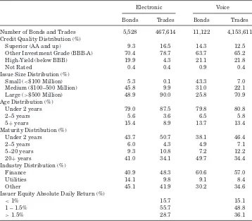
5,528 bonds. Following Edwards, Harris, and Piwowar’s (2007) categorization of bond characteristics, TableIshows that trading differs noticeably between the electronic and voice channels. Higher quality, younger, closer-to-maturity, non-financial industry, and larger issues are more likely to be traded electroni-cally.6Edwards, Harris, and Piwowar (2007) find that these types of bonds are
more liquid, suggesting that electronic trading is more concentrated in bonds we expect ex ante to be more liquid. It is also possible that greater electronic trading in these bonds is one source of their better liquidity. In addition to differences in the cross-sectional characteristics of bonds, Table Ireports the distribution of trading based on the issuer’s stock return volatility on the day of the bond trade.7This view captures uncertainty about the firm’s value, which
can reduce bond liquidity for adverse selection and inventory risk reasons. Electronic bond trades are less likely on days when the issuer’s stock volatility is high (the absolute value of the return is greater than 1.5%). This could be due to those days having lower bond liquidity or higher costs of delay in running an auction.
5This only includes trades with sufficient data for our trading cost estimation. Analyses of thinly traded corporate bonds typically limit their samples for data availability reasons. For example, one of the most comprehensive studies, Edwards, Harris, and Piwowar (2007), report that there is insufficient data to estimate trading costs for 20% of bonds.
Table I
Bond Characteristics
The table presents descriptive statistics based on a sample of all U.S. investment-grade and high-yield corporate bond trades in the Financial Industry Regulatory Authority’s (FINRA) Trade Reporting and Compliance Engine (TRACE) from January 2010 through April 2011, excluding all interdealer trades. Electronic refers to MarketAxess trades; Voice trades are all TRACE reported trades excluding electronic auction trades. High-yield is below BBB rated. Foreign issue bonds are excluded. All figures in the table other than the first row are percentages.
Electronic Voice
Bonds Trades Bonds Trades
Number of Bonds and Trades 5,528 467,614 11,122 4,153,611 Credit Quality Distribution (%)
Superior (AA and up) 9.3 16.5 14.3 12.5
Other Investment Grade (BBB-A) 70.4 78.7 63.7 65.2
High-Yield (below BBB) 19.9 4.3 21.1 21.8
Not Rated 0.4 0.4 0.9 0.4
Issue Size Distribution (%)
Small (<$100 Million) 5.3 0.1 43.3 7.0
Medium ($100–500 Million) 45.8 9.9 31.0 22.1
Large (>$500 Million) 48.9 90.0 25.8 70.9 Age Distribution (%)
Under 2 years 79.0 87.5 79.8 80.8
2–5 years 5.6 3.6 6.5 5.8
5+years 15.4 8.9 13.7 13.4
Maturity Distribution (%)
Under 2 years 43.7 50.7 38.1 46.4
2–5 years 6.0 4.3 4.9 7.1
5–20 years 9.3 10.8 7.2 12.2
20+years 41.0 34.1 49.7 34.4
Industry Distribution (%)
Finance 40.9 48.3 60.6 57.0
Utilities 14.1 9.8 9.1 8.4
Other 45.1 41.9 30.2 34.6
Issuer Equity Absolute Daily Return (%)
<1% 15.7 15.1
1 – 1.5% 55.7 48.8
>1.5% 28.7 36.1
II. Analytical Framework
in the OTC market. We permit search costs to differ by trade initiator so that the case of a corresponding sell order of the same size is not necessarily symmetric. Consider first a buy order and let p0 denote the trader’sexpectedpurchase price through bilateral voice trading in the OTC market. Correspondingly, let
padenote the expected price if the trader were instead to select the electronic auction. The trader selects the OTC market if the expected purchase price is lower, that is,p0< pa. We model the expected purchase price in OTC trading as the expected value of the asset, denoted byv, plus the expected dealer markup or premium, denoted byd(x), so thatp0=v+d(x). Herexis a vector that might include signed trade size as well as bond and market characteristics.8
Now consider the cost of trading in the auction mechanism. The trader can conduct an auction by simultaneously selecting M dealers to contact (up to a maximum of ¯M) and the auction’s duration. The choice of M is itself en-dogenous: contacting more dealers will generate more responses resulting in better prices but greater information leakage regarding trading intentions. The trade-off between competition and leakage will depend on market and trade characteristics. Similarly, a seller who chooses to run the auction longer may obtain a higher response rate but risk greater leakage of information. Condi-tional upon selecting the auction mechanism, the investor optimally sets the number of dealers to contact and the auction duration. We assume an interior solution and denote byM(x) this “reduced-form” function.9
LetNbe the (random) number of dealers responding givenM(x) dealers are queried. In our later empirical analysis, we will estimate the response function assuming a Poisson distribution for responses. We model E[N]=λ(x), where
λ(x) is the hazard rate that depends on bond and trade characteristics,x. The auction fails (i.e., no dealers respond, or they respond with uncompetitive bids) with probabilityq(x)=Pr[N=0]=e−λ(x). In this case, the trader is forced to enter into bilateral trading with a dealer and incurs a potential additional cost from information leakages(x)≥0 relative to the price had he or she first gone to the voice OTC market. Leakage refers to the revelation of trading intentions and includes the negative impact on price for subsequent orders in the same or related securities. The termsis positively related to trade size and can vary across traders. Thus, if there are zero responses, the total purchase price is
p0+s(x), where p0is the expected price in the OTC market.
With probability 1−q(x) the auction is viable. In a sealed bid auction, each dealer bids the expected value of the asset (v) plus a dealer-specific inventory term, denoted by π, which reflects compensation for unwanted risk. There may be cross-sectional dispersion in inventory across dealers. A dealer who has an opposite-side inventory position may aggressively bid to reduce risk, so
8For simplicity, we assume that execution obtains with certainty in a bilateral negotiation. It is straightforward to extend the model to allow for a positive probability that a negotiation leads to no trade, followed by subsequent searches in the future. See Duffie, Garleanu, and Pedersen (2005).
the inventory premium can be negative. The expected total auction price, pa, is thus
pa=q(p0+s(x))+(1−q(x))(v+π(x)), (1)
where π(x) is the expected inventory premium. Equation (1) yields the key trade-off where a trader chooses the OTC market if and only if
q(x)s(x)+
1−q(x)
(π(x)−d(x))>0, (2)
and the auction market otherwise. For a given trade size, the higher the costs of leakage s and the inventory premium π, the greater likelihood of trading OTC versus the electronic auction. The opposite is true for the dealer markup
d. Similarly, a lower dealer response rateλ(e.g., on less liquid issues) implies a higherqand hence less likelihood of selecting the auction. Equation(2)forms the basis for the endogenous choice model we estimate below.
The model allows for costs to vary with size in a nonlinear way. The observed execution price p(x) is the lower envelope of the cost curves reflecting the investor’s optimal venue choicek∈ {0,a}:
p(x)=min[p0(x|k=0),pa(x|k=a)]. (3)
For small sizes, leakagesis minimal and the electronic auction mechanism dominates. This is also the case if dealers are competitive in bidding so that
π(x) is very small. As trade size rises, we expect higher costs from leakage and so the dealer mechanism will dominate beyond a critical size. If the dealer markupd(x) reflects economies of scale or bargaining power, as the previous literature suggests, realized cost may decline withx.
Buy and sell orders need not be symmetric, especially in fixed income mar-kets where many bonds are bought and held to maturity, limiting their float and making short sales especially difficult.10Consequently, bond dealers may
signal their inventory to encourage buyers of specific issues to call them di-rectly, increasing investors’ preference for OTC for buyer-initiated trades. In addition, some sells may be forced liquidations or “fire sales,” where the cus-tomer seeks multiple bids to maximize the chances of completing the trans-action and to mitigate dealer market power, increasing OTC use for buys relative to sells. Let b(x) denote the price differential between a buy and the equivalent sale. The selection equation (2) for a sell order now becomes
q(x)s(x)+1
−q(x) π(x)−b(x)−d(x)
>0 so that, whenb>0, buys are more
likely to be traded by voice.
The framework also offers guidance regarding another real-world subject, namely, multiple bond issues by the same company. Multiple bond issues allow dealers to offset risks through substitution, lowering their inventory costs and hence the premiumπ, and increasing the response rateλ. If substitution effects were limited to risk reduction, we would expect that multiple-issue bonds have lower costs and are more likely to be traded in an electronic auction than
equivalent single-issue bonds. Conversely, from an information perspective, leakage s may be higher for multiple-issue bonds because dealers can trade other bonds by the same issuer, thereby offsetting the benefit of using an auction. The net impact of these effects on venue choice is thus an empirical question. Before turning to our analysis based on our framework of optimal venue selection, we develop our empirical approach to measuring trading costs.
III. Liquidity and Transaction Costs
A number of approaches have been used to calculate transaction costs in sparsely traded fixed income markets. Unlike equity markets, intraday bid and ask quotes for corporate bond markets are not readily available. The sim-plest approach is to compare roughly contemporaneous buy and sell prices of the same bond to impute a spread. As the TRACE data identify whether a transaction is buyer- or seller-initiated, imputed spreads are straightforward to compute. Hong and Warga (2000) follow this approach to estimate what Harris and Piwowar (2006) refer to as a benchmark methodology by subtract-ing the average price for all sell transactions from the average buy price for each bond each day when there is both a buy and a sell (see also Feldh ¨utter (2012)). In the Internet Appendix,11 we display trading costs in basis points
measured using the difference between average prices for all buy and sells for each bond for bond days when there is both a buy and a sell.
However, while imputed costs are simple, they have deficiencies. Given in-frequent trading in many bonds, the same bond same day criterion limits the amount of usable data. Harris and Piwowar (2006) and others use a regression approach to utilize more data. We employ the regression approach’s implicit assumption regarding interdealer trades to more closely follow the transac-tion cost literature in the equity markets to construct a cost of transacting foreach trade. This enables us to easily include cross-sectional and time-series covariates in our cost estimation and control for endogenous choice in venue se-lection. Beyond any obvious explicit costs (e.g., commissions and fees), we want to include bid-ask spread and market impact costs.12Accordingly, we compute
percentage transaction costs in basis points relative to a variety of benchmarks but focus here on the last trade in that bond in the interdealer market as most representative. Cost is defined as
Cost=ln
TradePrice
BenchmarkPrice
×Trade Sign, (4)
whereTrade Signtakes the value of+1 if the investor is buying and –1 if the investor is selling. We compute transactions costs throughout in basis points ofvalueby multiplying equation(4)by 10,000.
11The Internet Appendix may be found in the online version of this article on theJournal of
Financewebsite.
It is important to note that the cost in (4) is a fraction of trade value, not yield. As noted above, the trading convention for investment-grade corporate bonds is for negotiations to take place in terms of yield relative to the yield on a benchmark Treasury. From an investment perspective, cost should be expressed relative to the value of the trade to correctly reflect the full costs of trading, often referred to as implementation shortfall. We use the last in-terdealer price as the benchmark price.13Harris and Piwowar (2006),
Bessem-binder, Maxwell, and Venkataraman (2006), and Edwards, Harris and Piwowar (2007) calculate trading costs with regressions of the change in price between transactions on the change in the trade sign. Consistent with our approach, interdealer trades in these papers are given a trade sign of zero. Our approach uniquely assigns a cost to each transaction allowing for more straightforward inclusion of transaction-specific covariates of interest relating to the number of dealers queried and the number responding. The disadvantage of calculating a cost for each trade is the information in trade signs and price changes is less fully exploited. In addition, the interdealer price may include costs that dealers charge each other for trading.
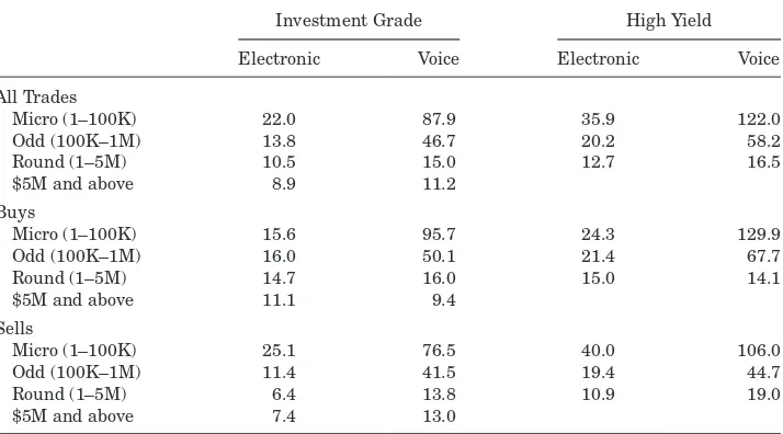
TableII presents transaction costs for electronic and voice trades by trade size for investment-grade and high-yield bonds overall and for buys and sells. The trade-size categories in TableIIare based on dollar value traded and chosen in accordance with standard industry conventions: micro ($1 to $100K), odd-lot ($100K to $1M), round-lot ($1M to $5M), and maximum reported size ($5M+) trades. Trade sizes in TRACE are capped at $5 million for investment-grade bonds and $1 million for high-yield bonds.14Investment-grade and high-yield
bonds differ in their trading convention as negotiation in investment-grade corporate bonds is in terms of the yield spread over a benchmark Treasury of similar duration whereas negotiations in high-yield bonds occur in terms of dollars. This difference in pricing convention means that dealers’ bids in high-yield bonds are exposed to broad interest rate risk between the time of placement and execution, so that auction time is more critical.
A steep decline in trading costs with trade size and substantial cost differ-ences between electronic and voice are evident. For investment-grade bonds, odd-lot electronic trades average 13.8 basis points, while for voice trades the cost is substantially higher at 46.7 basis points. The costs for voice trades fall to 10.5 and 8.9 basis points in the round-lot and maximum trade size categories, respectively. Electronic costs fall with trade size as well, albeit more slowly. These costs are similar in magnitude to previous estimates of corporate bond
13Using the last price introduces a bias from bid-ask bounce. Another popular benchmark, the Volume Weighted Average Price, suffers from similar issues when there are few trades in the day. We do not use the many interdealer trades that are paired with customer trades, that is, same bond, day, time, and quantity, as these may contain larger costs for interdealer trading.
Table II
Bond Trading Costs
The table presents estimates of one-way trading costs in basis points for a sample of all U.S. investment-grade and high-yield corporate bond trades in the Financial Industry Regulatory Au-thority’s (FINRA) Trade Reporting and Compliance Engine (TRACE) from January 2010 through April 2011. Electronic refers to MarketAxess trades; Voice trades are all TRACE reported trades excluding electronic auction trades. High-yield is below BBB rated.
Investment Grade High Yield
Electronic Voice Electronic Voice
All Trades
Micro (1–100K) 22.0 87.9 35.9 122.0
Odd (100K–1M) 13.8 46.7 20.2 58.2
Round (1–5M) 10.5 15.0 12.7 16.5
$5M and above 8.9 11.2
Buys
Micro (1–100K) 15.6 95.7 24.3 129.9
Odd (100K–1M) 16.0 50.1 21.4 67.7
Round (1–5M) 14.7 16.0 15.0 14.1
$5M and above 11.1 9.4
Sells
Micro (1–100K) 25.1 76.5 40.0 106.0
Odd (100K–1M) 11.4 41.5 19.4 44.7
Round (1–5M) 6.4 13.8 10.9 19.0
$5M and above 7.4 13.0
transaction costs. While electronic costs are lower than voice, Table I shows that the characteristics of bonds traded via the electronic and voice mecha-nisms differ, with bonds likely to be more liquid (e.g., bonds with larger issue sizes) trading more electronically.
As expected, trading costs in high-yield bonds are much higher than in investment-grade. The differentials are greatest in the smaller trade sizes. Comparing across voice and electronic markets for high-yield and investment-grade bonds, the differentials are large initially for smaller sizes but narrow as size increases. It is not obvious that there are systematic differences by trade side, although for voice it appears that buys are more costly than equivalent-sized sells. That is not the case in the electronic market.
The results in this section provide initial evidence on the relative costs of trading in an electronic auction versus sequentially negotiating with deal-ers. While TableIIcontrols for some differences in credit quality, which is an important component of potential endogeneity in investors’ choice of trading mechanism, a more rigorous multivariate approach is needed.
IV. Endogenous Venue Selection
TableIshows that electronic and voice trading differ on important bond char-acteristics and market conditions beyond credit quality. In addition, the choice of venue may depend on unobservable differences in trade characteristics. The standard econometric approach to control for unobservable characteristics of trades that affect both the costs of the trade and whether the trade is executed electronically is a two-stage switching model.15
A. Determinants of Trading Mechanism
In terms of our conceptual framework, define the cost for a purchase in venue
k as ck=(pk/v)−1, for k∈ {0,a}. We model expected costs as ck=z′δk+ηk, wherezis a vector of explanatory terms (including possibly nonlinear functions of size), and the error term η captures the unobserved costs of search and slippage, as detailed in the model. In stage 1, a trader chooses the lowest-cost venue. From equation(2), the auction venue is chosen if
ca≤c0 or z′(δ0−δa)+(η0−ηa)≥0 or z′δ+η≥0. (5)
This equation forms the basis of the probit equation in TableIII.
In stage 2, we model the true cost equation (if there is no selection bias) as
yk=x′βk+εk. (6)
The residual captures unobserved cost factors such as dealer inventory effects. Assuming joint normality,
E[y0|x,z,ca≥c0]=x′β0−ρ0σε0
ϕ(z′δ) 1−(z′δ) ≡x
′
β0−ρ0σε0mr0(z ′
δ) (7)
E[ya|x,z,ca≤c0]=x′βa+ρaσεa ϕ(z′δ)
(z′δ) ≡x ′β
a+ρaσεamra(z
′δ), (8)
where ρk is the correlation of εk andηk. Essentially, to run both regressions requires two Mill’s ratio variables (with appropriate dummies) where the de-nominators are slightly different (they sum to one).
B. Empirical Evidence on Venue Selection
Before estimating the probit first stage of the switching model, we return to the variables related to market conditions, bond characteristics, and trade size introduced in TableI. The dummy variablebuyis set to one if the investor buys and zero if the investor sells. The natural logarithm is taken of maturity (Maturity), bond age (Age), issue size (Issue Size), and the sum of the issue sizes of the issuer’s other bonds (Other Issue Size). The dummy variableMost Liquid denotes whether an issue is the most actively traded issue by that
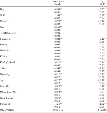
Table III
Venue Selection: Stage I Probit Model
The table provides probit models for the binary choice between electronic auctions and over-the-counter in investment-grade and high-yield bonds. The dependent variable is one if an electronic auction is selected; zero otherwise. Independent variables include dummy variables for the investor buying from a dealer,Buy, trade size,Oddlot ($100K–$1M),Roundlot ($1M–$5M), andMax
($5M+),A-BBB rating, industry (FinancialandUtility), and calendar time (Monday,Friday, and
End-of-month). The absolute value of the return on the issuer’s stock the day of the trade is|Ret|. Bond characteristics include the natural logarithm of the bond’s time to Maturity, time since issuance,Age,Issue Size, and issuer’sOther Issue Size. There is a dummy variable for the issuer’s
Most Liquidissue. All continuous independent variables are demeaned. Standard errors clustered on day and bond issue are in parentheses; ** and * denote statistical significance at the 0.01 and 0.05 level.
Investment High
Grade Yield
Buy −0.39** −0.51**
(0.01) (0.03)
Odd 1.00** 0.66**
(0.02) (0.04)
Round 0.70** −0.12*
(0.02) (0.05)
Max −0.46**
(0.02)
A-BBB Rating 0.04
(0.03)
Financial −0.24** −0.42**
(0.03) (0.06)
Utility 0.06 0.02
(0.04) (0.09)
Monday 0.03* 0.05*
(0.01) (0.02)
Friday −0.01 −0.03
(0.01) (0.02)
End-of-Month 0.21** 0.14**
(0.02) (0.02)
|Ret| −4.63** −2.94**
(0.36) (0.47)
Maturity −0.11** −0.11*
(0.02) (0.05)
Age −0.17** −0.10*
(0.02) (0.04)
Issue Size 0.22** 0.13**
(0.01) (0.03)
Other Issue Size −0.02** 0.01
(0.01) (0.00)
Most Liquid −0.08* −0.03
(0.04) (0.06)
Constant −1.25** −1.72**
(0.04) (0.05)
issuer. The trade size categories in Table IIare represented by Odd,Round, andMax. The dummy variableA-BBB Ratingis created for the lower quality investment-grade bonds, rated A through BBB. Issuer risk with significant time variation is proxied by|Ret|, defined as the absolute value of the issuer’s stock return that day. The calendar time dummiesMondayandFridayare used for the beginning and end of the week to capture inventory effects around the weekend, and dummies for the financial and utility sectors are also included as controls. A month-end dummy,End of Month, is one for the last trading day of the month and zero otherwise. Month-end trading is often related to index or rebalancing activity by institutions, so venue choice may differ.
We estimate the probit models for venue selection in TableIIIfor investment-grade and high-yield bonds, respectively. Standard errors control for contempo-raneous correlation across bonds on the same day and time-series correlation within bonds using the clustering approach of Petersen (2009) and Thompson (2011). All independent variables are demeaned to allow the trade-size dummy variables to be added together to calculate average trading costs in subsequent regressions. Consistent with TableI, larger issue size, younger, closer to ma-turity, and nonfinancial bonds are more likely to be traded electronically. Odd-and round-lot trades Odd-and bonds with larger issue sizes on Monday Odd-and at the end of the month are also more likely to be traded electronically. The smallest trades are most likely to be done by voice. Although most large investors use both electronic and voice, smaller retail-oriented traders may lack access to the auction platform, resulting in a smaller electronic market share in micro-sized trades. The calendar effects likely reflect greater opportunity costs of sequen-tial voice search on these days due to higher volumes (e.g., monthly rebalancing flows) and more intrinsic volatility (e.g., following the weekend).
The coefficient on the size of the issuer’s other bonds, Other Issue Size, is negative and significant for investment-grade bonds, indicating greater use of voice for bonds with multiple issues. In terms of the model, this is consistent with leakage costs arising from the ability to trade other bonds by the same issuer dominating the effect of lower inventory costs from better hedging. What is not clear is why the coefficient is not significant for high-yield bonds. This may reflect the much smaller sample size for auctions in high-yield bonds or the fact that the substitution effects of reduced risk but higher leakage offset each other in this category.
C. Regression Cost Estimates Controlling for Selection Bias
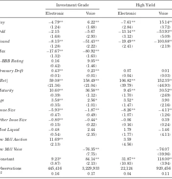
Table IV
Endogenous Selection of Trading Mechanism: Stage II Cost Model
In this table the probit specification in TableIIIis used to estimate the second-stage cost model for electronic auction and voice trades controlling for endogenous selection. Independent variables include dummy variables for the investor buying from a dealer (Buy), trade size (Oddlot ($100K– $1M),Roundlot ($1M–$5M), and Max ($5M+), and A-BBB rating. The absolute value of the return on the issuer’s stock the day of the trade is|Ret|. Bond characteristics include the natural logarithm of the bond’s time toMaturity, time since issuance (Age),Issue Size, and the issuer’s
Other Issue Size. There is a dummy variable for the issuer’sMost Liquidissue.Treasury Driftis the change in the yield in the benchmark Treasury at the time of the trade relative to yield at the time of the prior interdealer trade×Buy×years to maturity. All continuous independent bond variables are demeaned. The selectivity adjustment (Inverse Mill’s ratio) terms areInv Mill AuctionandInv Mill Voice. Standard errors clustered on day and bond issue are in parentheses; ** and * denote statistical significance at the 0.01 and 0.05 level.
Investment Grade High Yield
Electronic Voice Electronic Voice
Buy −4.79** 6.22** −7.61** 15.14**
(1.24) (1.68) (2.84) (3.72)
Odd −2.15 −5.67 −13.14** −53.93**
(1.68) (2.93) (3.12) (5.09)
Round −8.15** −51.43** −19.49** −100.88**
(1.28) (2.22) (2.41) (2.19)
Max −17.67** −80.92**
(1.32) (1.63)
A-BBB Rating 0.16 9.05**
(0.42) (1.46)
Treasury Drift 0.43** 0.23** 0.07 0.01
(0.01) (0.01) (0.04) (0.03)
|Ret| 59.08** 158.49** 106.82** 152.35**
(21.36) (21.04) (39.79) (46.93)
Maturity 10.60** 36.58** 9.45** 30.52**
(0.39) (1.12) (1.70) (2.69)
Age 3.58** 2.56* 3.52* 3.90
(0.35) (1.01) (1.47) (2.16)
Issue Size −5.93** −1.87** −8.26** −4.11**
(0.47) (0.49) (1.07) (1.26)
Other Issue Size −0.80** −0.44* −0.06 0.39
(0.15) (0.22) (0.16) (0.24)
Most Liquid −0.48 2.44 1.79 −1.46
(0.54) (2.35) (1.77) (4.11)
Inv Mill Auction 11.69** 3.59
(2.13) (4.56)
Inv Mill Voice −76.35** −76.07
(7.75) (39.96)
Constant 9.23* 84.14** 31.87** 118.00**
(3.87) (2.13) (10.83) (3.94)
Observations 445,416 3,229,933 22,124 920,456
are as described earlier. As before, all continuous independent variables are demeaned. The selectivity adjustment (Mill’s ratio) terms in equations(7)and
(8)areInv Mill VoiceandInv Mill Electronic, respectively.
The differences in size coefficients between the voice and electronic columns show that the relative advantage of the two types of trading depends on bond and market characteristics. The difference in independent variable coefficients (electronic minus voice) shows that the relative costs of electronic auctions decrease in issue size and increase in age, consistent with easier trades being done in electronic auctions. The inverse Mills ratio term for voice trades has a negative coefficient, consistent with our model of selection, which suggests that the voice market is chosen for orders with a higher likelihood of leakage and higher search costs. The omitted trade-size dummy variable is for the smallest trades. Therefore, the coefficients on other trade-size dummy variables represent differences in cost relative to the smallest trade size. Adding the intercept to the trade-size variable and incorporating the average inverse ratio term gives the selectivity-adjusted expected trading costs for an average trade in each trade size across the mechanisms.
For the smallest trade size in investment-grade bonds with the average bond and market characteristics, the expected trading cost is 67 basis points when using voice and 31 basis points when using the electronic mechanism. The difference between these estimates is narrower than the difference in Table II, but still substantial. The trade-size coefficients differ significantly between electronic and voice. For odd-lot trades the expected trading cost is 62 basis points when using voice and 29 basis points when using the electronic mechanism. The coefficients suggest that, for the two smallest trade sizes, trades with average characteristics are cheaper to execute electronically and the largest trades are cheaper to execute by voice.
The cost differentials are noteworthy for the smaller-sized trades. Clearly, the auction mechanism is preferred for this size over the OTC alternative. Given the relative size of the costs, the slippage term sor the probability of nontradingqwould need to be implausibly large to explain this selection. It is likely that this result reflects some of the differences in investor composition across the venues referred to earlier. Specifically, the results may reflect the fact that smaller and less active traders who could benefit from trading their odd lots in an auction framework are unwilling to bear the associated setup costs, closing out this option. It is also possible that voice is selected for small trades because of speed, research services, or broker relationships.
The value of optimal venue selection provides an opportunity to roughly as-sess the economic impact of the introduction of electronic auctions into an OTC environment. A conservative measure of the value from electronic auctions,
V(x), is the maximum of zero and the cost differential (weighted by volume of trade) between the voice and auction mechanisms, multiplied by the trading volume in that size category:
In other words, the calculation assumes that the default mechanism is OTC and asks how much could be gained from trading at a lower-cost auction if optimal. This calculation is conservative because the resulting value ignores the possible impact of auction competition on dealer quotes in the OTC market and further excludes any gains from the ability to trade more. Summing across all trade-size ranges yields the aggregate value of the auction mechanism.
Overall, we estimate that the auction mechanism could result in potential cost savings of at least $2 billion per annum on $1.4 trillion in trading volume. These savings should be reflected in higher realized investment returns to the ultimate investors of the bonds. Again, this is a conservative annual estimate and is likely to grow over time as the range of order sizes over which the elec-tronic auction mechanism dominates increases. Note that there are clear dif-ferences in the drift term coefficient between investment-grade and high-yield bonds, with the former positive and significant and the latter insignificant. One would expect such discrepancies because of differences in trading convention and more liquid bonds may well have greater loadings on the aggregate bond market, that is, less idiosyncratic noise.
The above analysis does not consider the costs of unfilled orders. SectionV
explores such costs for electronic auctions. We do not observe phone searches not resulting in trades, so a direct comparison across mechanisms for unfilled orders is not possible. In general, fully capturing expected trading costs across venues requires an experimental design where orders are randomly sent to different mechanisms. This study thus suffers from a shortcoming common to all studies of observed transaction costs.
D. Price Discovery and Permanent Price Impact
In addition to trading cost/liquidity, there are other measures of market qual-ity. An important consideration is price discovery. In particular, price changes can be decomposed into permanent (both public and private information re-lated) and transitory (liquidity) components. The transitory component largely reflects the trading costs measured above, so we focus on the permanent or information component of trading. There is no reason a priori to think that price pressure effects are different across the mechanisms as trades occur with the same intermediaries. However, the eventual information impact may be more clearly discerned by the market through one mechanism over another.
TableVreports regressions with the same control variables as in TableIV
Table V
Permanent Impact for Investment-Grade and High-Yield Bonds
The table presents the permanent impact, calculated similarly to the costs in equation (1) with the difference being that the trade price is replaced by the next benchmark price from an interdealer trade. Thus, if the trade is a buy and the next interdealer trade price is higher than the interdealer trade price preceding the trade, then the price impact is positive.Treasury Driftis the change in the benchmark treasury’s yield at the time of the next interdealer trade relative to yield at the prior interdealer trade×Buy× years to maturity. See TablesIIIandIVfor definitions of independent variables. In addition, the trade-size dummy variables are interacted with a dummy variable for electronic auction trades All continuous independent bond variables are demeaned. Standard errors clustered on day and bond issue are in parentheses; ** and * denote statistical significance at the 0.01 and 0.05 level.
Investment High
Grade Yield
Buy 4.74** 14.81**
(0.76) (1.98)
Odd −0.89** 0.14
(0.17) (0.66)
Round 2.10** 7.78**
(0.25) (1.07)
Max 3.00**
(0.26)
Auction*Micro 1.33** 4.24**
(0.19) (1.24)
Auction*Odd 2.88** 5.36**
(0.26) (1.26)
Auction*Round 0.91* −4.92*
(0.37) (2.20)
Auction*Max 1.06
(0.88)
A-BBB Rating −0.39*
(0.16)
Treasury Drift 0.28** −0.03
(0.01) (0.02)
|Ret| −8.89 −14.23
(8.77) (28.73)
Maturity −0.22 −0.36
(0.20) (0.80)
Age 0.29* −0.60
(0.14) (0.68)
Issue Size −0.29* 0.38
(0.13) (0.44)
Other Issue Size −0.11 0.01
(0.06) (0.07)
Constant −2.37** −9.38**
(0.44) (1.42)
Observations 3,216,546 824,483
interdealer benchmark trades used for calculating permanent price impacts. We interact the electronic auction dummy variableAuctionwith the trade size dummies to measure differences in price impact between the two mechanisms for each trade-size category.
TableVimplicitly decomposes the total price impact in TableIVinto its per-manent and transitory components. The transitory price impact is profit for the dealer while the permanent impact is interpreted as information impounded into price. Duffie, Giroux, and Manso (2010) model how information diffusion increases in the number of contacts traders make. If auctions expose trading intentions to more counterparties, then auctions should have a higher price impact. This is consistent with our model’s assumption that leakage of infor-mation increases in the number of dealers contacted. TableVshows that larger trades, buys, and smaller issues have larger price impacts. TableIIIshows that these characteristics lead to less electronic trading. Electronic trades thus have larger price impact, although the statistical significance fades in larger trade sizes.
V. Trading and Bidding Behavior in Electronic Auctions
As in our model, theory suggests that bidders’ participation is crucial for auc-tion performance (for example, Bulow and Klemperer (2009)). We next turn to detailed data on dealers’ bidding behavior and responses in electronic auctions. Our model predicts that factors that increase the probability of dealers bidding in an electronic auction should be the same factors that lead investors to choose an electronic auction over voice search. We first examine dealers’ bidding re-sponses to auctions. We then use those expected response rates to study how the response rates impact trading costs in the electronic auction. Finally, we provide evidence on the costs of auctions that fail to trade in repeated attempts electronically and the costs of completing the trade over the phone.
A. Dealers Bidding in Auctions
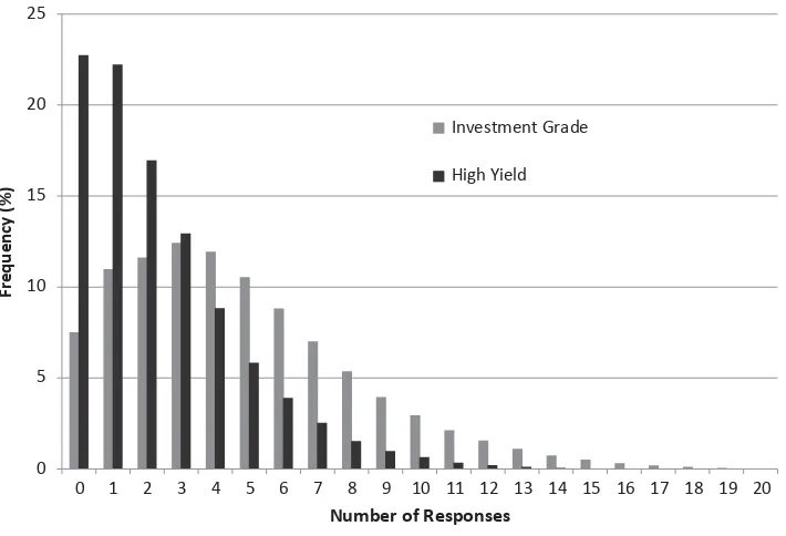
Figure 1 illustrates the frequency distribution of the number of dealer re-sponses in the auction market for investment-grade and high-yield bonds. For investment-grade bonds the modal response is three. With that number of dealers, the typical auction should approach a competitive outcome. In 7.3% of auctions, no dealers respond. Auctions in high-yield bonds have fewer dealers responding, with the modal number being zero and the next most frequent outcome being one bid. In roughly 60% of high-yield auctions there are two or fewer bids, suggesting that dealers’ propensity to bid may explain the low auction market share in these bonds.
0
Figure 1. Frequency distribution of dealer responses.The figure shows the frequency dis-tribution of the number of dealer responses in all electronic auctions in the sample, broken down for investment-grade and high-yield bonds. Data are from January 2010 through April 2011, excluding all interdealer trades.
The difference in dealers queried is not nearly enough to fully explain the lower the number of bids compared to investment-grade bonds. The response rate is about half as large in high-yield bonds. This leads to more high-yield auctions receiving no responses and fewer orders being filled.
For investment-grade bonds, the number of dealers queried decreases with trade size, which is consistent with leakage increasing in trade size. However, the numbers of dealers responding increases in trade size, that is, dealers are more likely to respond for large trades. The percentage of dealers responding increases substantially from 15.7% for the smallest trades to 28.9% for the largest trades. These results correspond to dealers’ cost of participation being fixed across auctions, so the participation cost per bond declines in trade size. Alternatively, large trades are done in bonds where dealers are more likely to respond. While dealers’ response rates increase with trade size, the fraction of auctions with no response also increases in trade size. This implies that dealers’ decisions to bid in particular auctions are not independent and bonds, trades, or market characteristics affect bidding propensity across dealers.
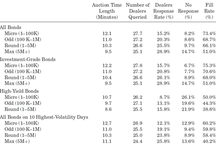
Table VI
Descriptive Statistics for Number of Dealers in an Auction
The table presents descriptive statistics from January 2010 through April 2011 for the length of time (in minutes) the auction is run, the number of dealers participating in electronic auctions, and the percentage of auctions that resulted in a trade. Four trade size categories by dollar size are represented, based on market conventions, up to a maximum of $5M and above. The 10 highest-volatility days are identified as the 10 days with the highest absolute CRSP value-weighted return. Figures reported are sample means.
Auction Time Number of Dealers No Fill Length Dealers Response Response Rate (Minutes) Queried Rate (%) (%) (%)
All Bonds
Micro (1–100K) 12.1 27.7 15.2% 8.2% 73.4%
Odd (100 K–1M) 11.0 27.2 20.3% 8.6% 68.7%
Round (1–5M) 10.3 26.6 25.5% 9.7% 66.1%
Max (5M+) 9.5 25.1 28.9% 14.7% 51.0%
Investment-Grade Bonds
Micro (1–100K) 12.2 27.8 15.7% 6.7% 75.3%
Odd (100 K–1M) 11.0 27.2 20.8% 7.7% 70.6%
Round (1–5M) 10.4 26.6 26.1% 8.9% 68.0%
Max (5M+) 9.5 25.1 28.9% 14.7% 51.0%
High-Yield Bonds
Micro (1–100K) 10.7 26.2 8.7% 26.1% 50.0%
Odd (100 K–1M) 9.7 27.1 13.1% 19.6% 44.3%
Round (1–5M) 8.6 25.5 15.8% 21.9% 38.6%
All Bonds on 10 Highest-Volatility Days
Micro (1–100K) 12.7 26.9 12.1% 12.9% 60.2%
Odd (100 K–1M) 11.0 25.5 19.1% 9.4% 59.8%
Round (1–5M) 10.3 25.0 23.8% 8.9% 58.4%
Max (5M+) 11.1 24.4 25.8% 13.6% 40.2%
rates are low when auctions are unlikely to get any dealer bids, and auctions with at least one dealer bid often do not result in a trade. The likelihood of the joint event that an auction receives a bid but no trade occurs is increasing in trade size. This last fact implies that investors are more sensitive to costs in larger trades, or bids are relatively less competitive in large trades. High-yield bonds exhibit similar properties with response rates increasing in trade size. Dealers are less likely to bid in high-yield bonds, resulting in less competition and more failed auctions. While fill rates range from 50% to 75% for different trade sizes in investment-grade bonds, fill rates are 50% or below for all trade sizes in high-yield bonds.
Almost all auctions are 5, 10, 15, or 20 minutes, with the approximate per-centages being 20, 50, 10, and 20, respectively.16Auctions for larger trades run
for shorter periods, consistent with greater information leakage concerns. This is also consistent with a higher response rate from dealers for larger orders. Auctions are short for high yield bonds, likely due to their lower liquidity and greater scope for information leakage.
Longer auctions allow dealers more time to bid, presumably increasing par-ticipation. However, auction length could also be associated with unobservable factors that proxy for more difficult trading conditions, which in turn induce lower dealer bidding. To examine this issue (and move beyond the simple aver-ages in TableVI), we model the number of dealersN(N=0,1,2 . . . ) respond-ing toMqueries, controlling for bond, trade, and market characteristicsz, as
E[N|M]=λ(z). Given that the number of dealers is integer valued, we esti-mate a count data model. This design also naturally allows for zero outcomes or auction failure. In particular, we model tradeias the outcome of a Poisson distribution with conditional mean,
ln (λi)=z
′
iβ+ui, (10)
where the error termui captures individual (unobserved) variation in dealer responses. It is important to allow for cross-sectional heterogeneity in estima-tion because our conceptual framework suggests that bargaining power and leakage vary across traders. When ui has a gamma distribution Ŵ(1, θ), this yields a negative binomial model. Unlike the Poisson model, we do not restrict the mean and variance of the sample data to be equal. Overdispersion (the variance exceeds the mean) is quite common with count data and hence the negative binomial is preferred. The distribution of the number of dealer re-sponses Ni in auctioniconditioned onzi is
P(Ni=ni|zi)=
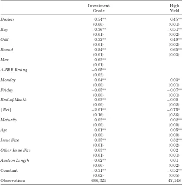
Table VII reports estimates of the dealer response model for investment-grade and high-yield bonds.
The log of the number of dealers is strongly positive as expected. Buy orders are less likely to have responses, consistent with short sale difficulties. This result is more apparent in high-yield bonds. The model can help traders better predict auction interest to utilize this mechanism more efficiently and reduce costs. The probability of the auction failing (with no responses at all) is
P(Ni=0|zi)=
θ
θ+λi θ
, (12)
which is the analog to the Poisson probability with no heterogeneity in re-sponses. There is a marked jump in the probability of auction failure as trade
Table VII
Negative Binomial Model for Number of Dealers Responding in Auction
The table presents regression models for the number of dealers responding for a sample of electronic auctions from January 2010 to April 2011. The logarithm of the length of the auction in minutes and the number ofDealerssent a request for a quote in the auction is included. See TablesIII
andIVfor definitions of the other independent variables. All continuous independent variables are demeaned. Standard errors clustered on day and bond issue are in parentheses; ** and * denote statistical significance at the 0.01 and 0.05 level.
Investment High
Grade Yield
Dealers 0.54** 0.45**
(0.00) (0.01)
Buy −0.36** −0.51**
(0.01) (0.02)
Odd 0.32** 0.49**
(0.01) (0.02)
Round 0.54** 0.65**
(0.01) (0.03)
Max 0.62**
(0.01)
A-BBB Rating −0.05**
(0.02)
Monday 0.04** 0.03*
(0.00) (0.01)
Friday −0.05** −0.07**
(0.00) (0.01)
End-of-Month 0.02** −0.00
(0.00) (0.02)
|Ret| −2.01** −0.75*
(0.16) (0.36)
Maturity 0.02** 0.02**
(0.00) (0.00)
Age 0.01** 0.05**
(0.00) (0.00)
Issue Size 0.35** 0.32**
(0.01) (0.02)
Other Issue Size 0.03** 0.02
(0.01) (0.01)
Auction Length −0.02** 0.01
(0.00) (0.02)
Constant −0.31** −0.52**
(0.02) (0.05)
Observations 606,325 47,148
-10 0 10 20 30 40 50 60
20 19 18 17 16 15 14 13 12 11 10 9 8 7 6 5 4 3 2 1
Cost in Basis Points
Number of Resposes
Investment Grade
High Yield
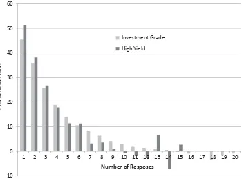
Figure 2. Transaction costs in basis points and number of dealers responding.The figure shows costs in basis points by the number of dealer responses in all electronic auctions in the sample with at least one response, broken down for investment-grade and high-yield bonds. Data are from January 2010 through April 2011, excluding all interdealer trades.
log number of dealers is less than one, which corresponds to the probability of dealers responding decreasing in the number of dealers queried. Larger trade size and issue size are positive predictors. Longer auctions are associated with more bidding in high-yield bonds, but not in investment-grade.
B. Trading Costs and Dealer Bidding
Auction theory predicts that the number of bids should be closely linked to the auction outcome. Figure2shows the costs in basis points as a function of the number of responding dealers for investment-grade and high-yield bonds. Competition lowers costs as is clear from the figure. For investment-grade bonds, when only a few dealers respond costs are high, ranging from 24 to 45 basis points. The mean realized costs approach 0 as the number of responses begins to exceed 10. This result is consistent with some dealers willing to price aggressively to liquidate unwanted inventory. The low realized costs could also result from dealers suffering from the winner’s curse.
Table VIII
Corporate Bond Trading Costs in an Auction Mechanism
The table presents regression models for trading costs for electronic auctions. The logarithm of the number ofExpected Dealer BidsandUnexpected Dealer Bidsbased on the estimates in TableVII
are included. See TablesIIIandIVfor definitions of the other independent variables. All continuous independent bond variables are demeaned. Standard errors clustered on day and bond issue are in parentheses; ** and * denote statistical significance at the 0.01 and 0.05 level.
Investment High
Grade Yield
Buy −4.07** −10.12**
(0.94) (2.44)
Odd −7.84** −9.49**
(0.39) (1.97)
Round −8.86** −9.42**
(0.51) (2.98)
Max −5.74**
(0.95)
A-BBB Rating 1.34**
(0.46)
Treasury Drift 0.44** 0.07
(0.01) (0.04)
|Ret| 91.68** 109.47**
(15.34) (36.87)
Maturity 0.76** 0.61**
(0.04) (0.19)
Age 0.09 0.49
(0.07) (0.38)
Issue Size −5.69** −6.98**
(0.40) (1.70)
Other Issue Size −0.43* −0.60
(0.19) (0.91)
Expected Dealer Bids −11.58** −17.08**
(0.68) (3.24)
Unexpected Dealer Bids −96.98** −134.26**
(4.28) (27.39)
Constant 360.36** 517.18**
(14.41) (95.38)
Observations 437,591 21,914
R2 0.19 0.06
conditional on the number of bids is much smaller than the unconditional differences shown in TableII. This result demonstrates that the lower response rates in Figure1and TableVIlargely explain the higher costs for high-yield bonds.
TableVIIIpresents cost estimates for the auction market incorporating the number of dealer bids.17 The estimates show that the finding that costs are
decreasing in the number of dealers responding (Figure 2) is robust to the
inclusion of bond and trade characteristics. Essentially, Table VIII can be thought of as a regression with the log of frequency response as an explanatory variable. We use the natural logarithm of the bids because Figure2 shows a clear nonlinearity in costs as a function of bids. The model decomposes the number of bidders into the expected and unexpected number of bidders from the negative binomial dealer response model in Table VII. The logarithm of expected and unexpected responses is taken after subtracting the overall mini-mum and adding one, ensuring that the minimini-mum of the logarithms of expected and unexpected responses is zero before demeaning. The coefficient on the un-expected number of bidders is significantly more negative than the coefficient on the expected number, showing that an unexpectedly lower number of bid-ders responding is particularly costly. The high costs of an unexpectedly lower number of bids could result from dealers being less likely to bid at times when liquidity is lower.
Interestingly, the costs of trading are no longer monotonically decreasing in trade size once we condition on the number of bids, demonstrating that dealer bidding behavior drives the decline in costs for larger trades. This finding enhances the standard argument that costs decrease in trade size because investors’ bargaining power increases with trade size.18 Our results suggest
that a source of declining dealer market power is greater bidding competition for larger trades. If dealer behavior is similar in the voice market, then the same effect should be present. TableVIIIalso shows that the cost differences between investment-grade and high-yield bonds are largely driven by dealer bidding behavior. The inclusion of the dealer bidding variables in TableVIII
makes the difference in trading costs between investment-grade and high-yield bonds in TablesIIandIVshrink to close to zero. This suggests that the trade, bond, and market characteristics that drive differences in liquidity in electronic auctions operate through their impact on dealer bidding behavior.
C. Failed Auctions and Trading Costs
The analysis of trading costs thus far does not capture the opportunity cost associated with the time to trade or the cost of failed trades. This is common as the data required to make such inferences are rarely present, and not present for the voice trades from TRACE. However, for the MarketAxess trades, we have information about auctions that did not lead to trades. Comparing Ta-blesVIIandVIIIshows that of the 609,455 auctions in investment-grade bonds, 438,829 or about 72% resulted in trades. For high-yield bonds only 21,887 or 46% of the 47,396 auctions led to trades. When the auction does not lead to a trade, the investor can give up, attempt another auction, or try to bilaterally negotiate a trade with a dealer. In this subsection, we attempt to quantify the costs after electronic auctions that did not lead to trade. A significant challenge
Table IX
Regression Models of Costs Incorporating Unfilled Auctions
The table reports the costs of electronic auctions including failed electronic auction inquiries, defined as auctions that ended up with no trade occurring in that auction. The first dummy variable,Repeat Auction,is for an electronic auction trade where there is a failed auction inquiry by the same investor, bond, day, size, and buy/sell direction. The second dummy,Auction Voice,is for an inquiry that did not result in a trade, where the cost is the cost in TRACE for the same bond, day, size, and buy/sell direction; we assume that the investor on Market Axess would have gotten this price going to the voice channel. See TablesIIIandIVfor definitions of the other independent variables. All continuous independent bond variables are demeaned. Standard errors clustered on day and bond issue are in parentheses; ** and * denote statistical significance at the 0.01 and 0.05 level.
Investment High
Grade Yield
Repeat Auction 2.51** 6.50*
(0.63) (2.54)
Auction Voice 11.61** 24.79**
(0.55) (1.99)
Buy −1.63 −3.02
(0.98) (2.14)
Odd −11.94** −17.23**
(0.43) (1.43)
Round −16.37** −23.40**
(0.56) (2.31)
Max −17.24**
(1.02)
A-BBB Rating 0.88*
(0.44)
Treasury Drift 0.43** 0.04
(0.01) (0.04)
|Ret| 127.97** 185.20**
(16.66) (36.22)
Maturity 0.92** 0.92**
(0.03) (0.19)
Age 0.77** 0.62*
(0.07) (0.29)
Issue Size −6.99** −7.91**
(0.37) (1.46)
Other Issue Size −0.66** −1.00
(0.20) (0.82)
Constant 24.32** 33.78**
(0.78) (2.07)
Observations 469,125 26,313
R2 0.15 0.05
is that our data do not unambiguously identify future trades linked to auctions that do not result in an immediate trade.
ended in a trade. We construct the dummy variableRepeat Auctionto identify these auctions. For the remaining electronic auctions that do not lead to an immediate trade, we look for a voice trade in the same bond, on the same day, on the same side, and for the same quantity. We find 34,273 such auctions/trades for which we set the dummy variable Auction Voiceequal to one. We use the trading cost for these trades as the cost associated with that auction.
Table IXreports cost regressions analogous to those in Table VIIwith the dummy variables described above and the additional observations where the trading costs for the corresponding voice trade are used for auctions without trades. Table IXshows that, for investment-grade bonds, repeated auctions have transaction costs that are on average 2.5 basis points higher than auctions leading to an immediate trade. For auctions without trades, the corresponding voice cost is 11.6 basis points higher than auctions with electronic trades. These effects are more than twice as large for high-yield bonds.
VI. Conclusion
The continued growth of electronic trading is an important driver of changes in liquidity, trading costs, and risk-sharing ability. Using a large sample of cor-porate bond transactions, we analyze the types of bonds, trades, and market conditions when electronic auctions offer lower costs and are chosen over voice negotiations. Electronic auctions are preferred for more active, liquid securi-ties or trades where the cost of leakage is lower and dealers are more likely to bid.
The approach here has many investment applications. Institutions and hedge funds can use our cost estimates to gauge the profitability and capacity of in-vestment strategies. Often a strategy may appear profitable on paper only to have the “alpha” dissipate in implementation or fail to reach an econom-ical scale due to market impact costs. Estimates by mechanism type can also be used by buy-side traders to improve their venue selection depend-ing on bond and market characteristics. The results confirm the value to traders and investors from sourcing liquidity widely and optimally selecting venue.
structure and fixed income markets by allowing traders to more easily engage in multilateral trading.19
Our results indicate that electronic auction markets are a viable and im-portant source of liquidity even in inactively traded instruments, although the benefits are concentrated in the most liquid bonds and in the easiest trades. Auction-like systems may add considerable value in liquid fixed income prod-ucts such as to-be-announced (TBA) mortgage-backed securities. Overall, we estimate that the option to trade corporate bonds in an electronic auction im-proves prices with an annual savings of $2 billion. This figure is likely to increase over time and represents a transfer from dealers to the ultimate in-vestors in these bonds.
Growing awareness of the magnitude of trading costs in fixed income mar-kets is spurring further market structure innovation. For example, both buy-and sell-side institutions buy-and existing trading venues are developing electronic crossing systems to directly match buyers and sellers of bonds. From a pub-lic popub-licy perspective the electronic auction mechanism offers a possible path through technological advances from an OTC structure to centralized, continu-ous trading. These are important considerations for recent regulations such as Dodd-Frank that seek to force significant derivatives trading from OTC onto centralized exchanges.
Initial submission: September 4, 2012; Final version received: January 24, 2014 Editor: Campbell Harvey
REFERENCES
Asquith, Paul, Andrea Au, Thomas Covert, and Parag Pathak, 2011, The market for borrowing corporate bonds, Working paper, MIT.
Barclay, Michael, Terrence Hendershott, and Kenneth Kotz, 2006, Automation versus intermedi-ation: Evidence from Treasuries going off the run,Journal of Finance61, 2395–2414. Barclay, Michael, Terrence Hendershott, and Timothy McCormick, 2003, Competition among
trad-ing venues: Information and tradtrad-ing on electronic communications networks,Journal of Fi-nance58, 2637–2666.
Bernhardt, Dan, Vladimir Dvoracek, Eric Hughson, and Ingrid M. Werner, 2005, Why do larger orders receive discounts on the London Stock Exchange? Review of Financial Studies18, 1343–1368.
Bessembinder, Hendrik, and Herbert M. Kaufman, 1997, A cross-exchange comparison of execution costs and information flow for NYSE-listed stocks,Journal of Financial Economics46, 293– 319.
Bessembinder, Hendrik, and William Maxwell, 2008, Transparency and the corporate bond market,
Journal of Economic Perspectives22, 217–234.
Bessembinder, Hendrik, William Maxwell, and Kumar Venkataraman, 2006, Market transparency, liquidity externalities, and institutional trading costs in corporate bonds,Journal of Financial Economics82, 251–288.