䊏
䊏
䊏
䊏
䊏
䊏
䊏
䊏
䊏
䊏
䊏
Queuing Theory
Each of us has spent a great deal of time waiting in lines. In this chapter, we develop mathe-matical models for waiting lines, or queues. In Section 20.1, we begin by discussing some ter-minology that is often used to describe queues. In Section 20.2, we look at some distributions (the exponential and the Erlang distributions) that are needed to describe queuing models. In Section 20.3, we introduce the idea of a birth–death process, which is basic to many queu-ing models involvqueu-ing the exponential distribution. The remainder of the chapter examines sev-eral models of queuing systems that can be used to answer questions like the following:
1 What fraction of the time is each server idle?
2 What is the expected number of customers present in the queue? 3 What is the expected time that a customer spends in the queue?
4 What is the probability distribution of the number of customers present in the queue? 5 What is the probability distribution of a customer’s waiting time?
6 If a bank manager wants to ensure that only 1% of all customers will have to wait more than 5 minutes for a teller, how many tellers should be employed?
20.1
Some Queuing Terminology
To describe a queuing system, an input process and an output process must be specified. Some examples of input and output processes are given in Table 1.
The Input or Arrival Process
The input process is usually called the arrival process.Arrivals are called customers.In all models that we will discuss, we assume that no more than one arrival can occur at a given instant. For a case like a restaurant, this is a very unrealistic assumption. If more than one arrival can occur at a given instant, we say that bulk arrivalsare allowed.
Usually, we assume that the arrival process is unaffected by the number of customers present in the system. In the context of a bank, this would imply that whether there are 500 or 5 people at the bank, the process governing arrivals remains unchanged.
future. Models in which arrivals are drawn from a small population are called finite source models.Another situation in which the arrival process depends on the number of customers present occurs when the rate at which customers arrive at the facility decreases when the facility becomes too crowded. For example, if you see that the bank parking lot is full, you might pass by and come another day. If a customer arrives but fails to enter the system, we say that the customer has balked.The phenomenon of balking was de-scribed by Yogi Berra when he said, “Nobody goes to that restaurant anymore; it’s too crowded.”
If the arrival process is unaffected by the number of customers present, we usually de-scribe it by specifying a probability distribution that governs the time between successive arrivals.
The Output or Service Process
To describe the output process (often called the service process) of a queuing system, we usually specify a probability distribution—the service time distribution—which governs a customer’s service time. In most cases, we assume that the service time distribution is independent of the number of customers present. This implies, for example, that the server does not work faster when more customers are present.
In this chapter, we study two arrangements of servers: servers in paralleland servers in series.Servers are in parallel if all servers provide the same type of service and a cus-tomer need only pass through one server to complete service. For example, the tellers in a bank are usually arranged in parallel; any customer need only be serviced by one teller, and any teller can perform the desired service. Servers are in series if a customer must pass through several servers before completing service. An assembly line is an example of a series queuing system.
Queue Discipline
To describe a queuing system completely, we must also describe the queue discipline and the manner in which customers join lines.
The queue disciplinedescribes the method used to determine the order in which cus-tomers are served. The most common queue discipline is the FCFS discipline(first come, first served), in which customers are served in the order of their arrival. Under the LCFS discipline(last come, first served), the most recent arrivals are the first to enter service. If we consider exiting from an elevator to be service, then a crowded elevator illustrates an LCFS discipline. Sometimes the order in which customers arrive has no effect on the
or-T A B L E 1 Examples of Queuing Systems
Situation Input Process Output Process
Bank Customers arrive at bank Tellers serve the customers
Pizza parlor Requests for pizza delivery Pizza parlor sends out
are received truck to deliver pizzas
Hospital blood bank Pints of blood arrive Patients use up pints of blood
Naval shipyard Ships at sea break down Ships are repaired and and are sent to shipyard return to sea
der in which they are served. This would be the case if the next customer to enter service is randomly chosen from those customers waiting for service. Such a situation is referred to as the SIRO discipline(service in random order). When callers to an airline are put on hold, the luck of the draw often determines the next caller serviced by an operator.
Finally, we consider priority queuing disciplines.A priority discipline classifies each arrival into one of several categories. Each category is then given a priority level, and within each priority level, customers enter service on an FCFS basis. Priority disciplines are often used in emergency rooms to determine the order in which customers receive treatment, and in copying and computer time-sharing facilities, where priority is usually given to jobs with shorter processing times.
Method Used by Arrivals to Join Queue
Another factor that has an important effect on the behavior of a queuing system is the method that customers use to determine which line to join. For example, in some banks, customers must join a single line, but in other banks, customers may choose the line they want to join. When there are several lines, customers often join the shortest line. Unfortunately, in many situations (such as a supermarket), it is difficult to define the shortest line. If there are sev-eral lines at a queuing facility, it is important to know whether or not customers are allowed to switch, or jockey, between lines. In most queuing systems with multiple lines, jockeying is permitted, but jockeying at a toll booth plaza is not recommended.
20.2
Modeling Arrival and Service Processes
Modeling the Arrival Process
As previously mentioned, we assume that at most one arrival can occur at a given instant of time. We define tito be the time at which the ith customer arrives. To illustrate this,
consider Figure 1. For i1, we define Titi1tito be the ith interarrival time. Thus,
in the figure, T1 8 3 5, and T2 15 8 7. In modeling the arrival process,
we assume that the Ti’s are independent, continuous random variables described by the
random variable A. The independence assumption means, for example, that the value of T2has no effect on the value of T3, T4, or any later Ti. The assumption that each Tiis
con-tinuous is usually a good approximation of reality. After all, an interarrival time need not be exactly 1 minute or 2 minutes; it could just as easily be, say, 1.55892 minutes. The as-sumption that each interarrival time is governed by the same random variable implies that the distribution of arrivals is independent of the time of day or the day of the week. This is the assumption of stationary interarrival times. Because of phenomena such as rush hours, the assumption of stationary interarrival times is often unrealistic, but we may of-ten approximate reality by breaking the time of day into segments. For example, if we were modeling traffic flow, we might break the day up into three segments: a morning rush hour segment, a midday segment, and an afternoon rush hour segment. During each of these segments, interarrival times may be stationary.
We assume that Ahas a density function a(t). Recall from Section 12.5 that for small
t, P(t At t) is approximately ta(t). Of course, a negative interarrival time is impossible. This allows us to write
P(Ac)
冕
c0
a(t)dt and P(Ac)
冕
∞c
L E M M A 1
We define l1 to be the mean or average interarrival time. Without loss of generality, we assume that time is measured in units of hours. Then l1 will have units of hours per ar-rival. From Section 12.5, we may compute l1 from a(t) by using the following equation:
l
1
冕
∞0
ta(t)dt (2)
We define lto be the arrival rate,which will have units of arrivals per hour.
In most applications of queuing, an important question is how to choose Ato reflect reality and still be computationally tractable. The most common choice for Ais the expo-nential distribution.An exponential distribution with parameter l has a density a(t) lelt. Figure 2 shows the density function for an exponential distribution. We see that a(t) decreases very rapidly for tsmall. This indicates that very long interarrival times are unlikely. Using Equation (2) and integration by parts, we can show that the average or mean interarrival time (call it E(A)) is given by
E(A) l
1
(3)
Using the fact that var AE(A2) E(A)2, we can show that
var A l
1
2 (4)
No-Memory Property of the Exponential Distribution
The reason the exponential distribution is often used to model interarrival times is em-bodied in the following lemma.
If Ahas an exponential distribution, then for all nonnegative values of tand h,
P(A t h|At) P(Ah) (5)
Proof First note that from Equation (1), we have
P(Ah)
冕
∞h
lelt[elt] h ∞
elh (6)
Then
P(A t h|At)
From (6),
P(Ath傽A t) el(th) and P(At) elt Thus,
P(Ath|At) e
e
l
(t
l
t h)
elh P(Ah) P(Ath傽At)
P(At) t1 = 3
T1 = 8 – 3 = 5 T2 = 15 – 8 = 7 t2 = 8 t3 = 15
F I G U R E 1
T H E O R E M 1
It can be shown that no other density function can satisfy (5) (see Feller (1957)). For reasons that become apparent, a density that satisfies (5) is said to have the no-memory property.Suppose we are told that there has been no arrival for the last thours (this is equivalent to being told that A t) and are asked what the probability is that there will be no arrival during the next hhours (that is, Ath). Then (5) implies that this prob-ability does not depend on the value of t, and for all values of t, this probability equals P(Ah). In short, if we know that at least ttime units have elapsed since the last arrival occurred, then the distribution of the remaining time until the next arrival (h) does not de-pend on t. For example, if h4, then (5) yields, for t5, t3, t2, and t0,
P(A9|A5) P(A 7|A3) P(A6|A2)
P(A4|A0) e4l
The no-memory property of the exponential distribution is important, because it implies that if we want to know the probability distribution of the time until the next arrival, then it does not matter how long it has been since the last arrival.To put it in concrete terms, sup-pose interarrival times are exponentially distributed with l6. Then the no-memory prop-erty implies that no matter how long it has been since the last arrival, the probability dis-tribution governing the time until the next arrival has the density function 6e6t. This means
that to predict future arrival patterns, we need not keep track of how long it has been since the last arrival. This observation can appreciably simplify analysis of a queuing system.
To see that knowledge of the time since the last arrival does affect the distribution of time until the next arrival in most situations, suppose that Ais discrete with P(A5)
P(A100) 12. If we are told that there has been no arrival during the last 6 time units, we know with certaintythat it will be 100 6 94 time units until the next arrival. On the other hand, if we are told that no arrival has occurred during the last time unit, then there is some chance that the time until the next arrival will be 5 1 4 time units and some chance that it will be 100 1 99 time units. Hence, in this situation, the distri-bution of the next interarrival time cannot easily be predicted with knowledge of the time that has elapsed since the last arrival.
Relation Between Poisson Distribution and Exponential Distribution
If interarrival times are exponential, the probability distribution of the number of arrivals occurring in any time interval of length tis given by the following important theorem.
Interarrival times are exponential with parameter lif and only if the number of ar-rivals to occur in an interval of length t follows a Poisson distribution with para-meter lt.
a(t) = e
t t
e t
F I G U R E 2
A discrete random variable Nhas a Poisson distribution with parameter lif, for n
0, 1, 2, . . . ,
P(Nn) e
n
l
!
ln
(n0, 1, 2, . . .) (7)
If Nis a Poisson random variable, it can be shown that E(N) var Nl. If we define
Ntto be the number of arrivals to occur during any time interval of length t, Theorem 1
states that
P(Ntn)
el n
t(
!
lt)n
(n 0, 1, 2, . . .)
Since Ntis Poisson with parameter lt, E(Nt) var Ntlt. An average of ltarrivals
occur during a time interval of length t, so lmay be thought of as the average number of arrivals per unit time, or the arrival rate.
What assumptions are required for interarrival times to be exponential? Theorem 2 pro-vides a partial answer. Consider the following two assumptions:
1 Arrivals defined on nonoverlapping time intervals are independent (for example, the number of arrivals occurring between times 1 and 10 does not give us any information about the number of arrivals occurring between times 30 and 50).
2 For small t (and any value of t), the probability of one arrival occurring between times tand t tis lto(t), where o(t) refers to any quantity satisfying
lim
t→0 o(
t t)
0
Also, the probability of no arrival during the interval between tand t tis 1 lt
o(t), and the probability of more than one arrival occurring between t and t t is o(t).
T H E O R E M 2
If assumptions 1 and 2 hold, then Ntfollows a Poisson distribution with parameter lt, and interarrival times are exponential with parameter l; that is, a(t) lelt.
In essence, Theorem 2 states that if the arrival rate is stationary, if bulk arrivals can-not occur, and if past arrivals do can-not affect future arrivals, then interarrival times will fol-low an exponential distribution with parameter l, and the number of arrivals in any in-terval of length tis Poisson with parameter lt. The assumptions of Theorem 2 may appear to be very restrictive, but interarrival times are often exponential even if the assumptions of Theorem 2 are not satisfied (see Denardo (1982)). In Section 20.12, we discuss how to use data to test whether the hypothesis of exponential interarrival times is reasonable. In many applications, the assumption of exponential interarrival times turns out to be a fairly good approximation of reality.
Using Excel to Compute Poisson and Exponential Probabilities
Excel contains functions that facilitate the computation of probabilities concerning the Poisson and exponential random variables.
The syntax of the Excel POISSON function is as follows:
■ POISSON(x,MEAN,TRUE) gives the probability that a Poisson random variable
■ POISSON(x,MEAN,FALSE) gives probability that a Poisson random variable
with mean Mean is equal to x.
For example, if an average of 40 customers arrive per hour and arrivals follow a Poisson distribution then the function POISSON(40,40,TRUE) yields the probability .542 that 40 or fewer customers arrive during an hour. The function POISSON(40,40,FALSE) yields the probability .063 thatexactly40 customers arrive during an hour.
The syntax of the Excel EXPONDIST function is as follows:
■ EXPONDIST(x,LAMBDA,TRUE) gives the probability that an exponential
ran-dom variable with parameter lassumes a value less than or equal to x.
■ EXPONDIST(x,LAMBDA,FALSE) gives the value of the density function for
an exponential random variable with parameter l.
For example, suppose the average time between arrivals follows an exponential distribu-tion with mean 10. Then l.1, and EXPONDIST(10,0.1,TRUE) yields the probabil-ity .632 that the time between arrivals is 10 minutes or less.
The function EXPONDIST(10,.1,FALSE) yields the height .037 of the density func-tion for x10 and l.1. See file Poissexp.xls and Figure 3.
Example 1 illustrates the relation between the exponential and Poisson distributions.
E X A M P L E 1
The number of glasses of beer ordered per hour at Dick’s Pub follows a Poisson distri-bution, with an average of 30 beers per hour being ordered.
1 Find the probability that exactly 60 beers are ordered between 10 P.M. and 12 midnight.
2 Find the mean and standard deviation of the number of beers ordered between 9 P.M.
and 1 A.M.
3 Find the probability that the time between two consecutive orders is between 1 and 3 minutes.
Solution 1 The number of beers ordered between 10 P.M. and 12 midnight will follow a Poisson
distribution with parameter 2(30) 60. From Equation (7), the probability that 60 beers are ordered between 10 P.M. and 12 midnight is
e6 6
0
0 6
! 060
Alternatively, we can find the answer with the Excel function POISSON(60,60,FALSE). This yields .051.
Beer Orders
F I G U R E 3
Poissexp.xls
3 4 5 6 7 8 9 10 11 12 13 14 15 16
C D E
Poisson Lambda
P(X=40) 40 0.541918
P(X<=40) 40 0.062947
Exponential
Lambda
P(X<=10) 0.1 0.632121
Density for X = 10 0.1 0.036788
2 We have l30 beers per hour; t4 hours. Thus, the mean number of beers ordered between 9 P.M. and 1 A.M. is 4(30) 120 beers. The standard deviation of the number of
beers ordered between 10 P.M. and 1 A.M. is (120)1/210.95.
3 Let Xbe the time (in minutes) between successive beer orders. The mean number of orders per minute is exponential with parameter or rate 3600 0.5 beer per minute. Thus, the probability density function of the time between beer orders is 0.5e0.5t. Then
P(1 X 3)
冕
3
1
(0.5e0.5t)dte0.5e1.5.38
Alternatively, we can use Excel to find the answer with the formula
EXPONDIST(3,.5,TRUE)EXPONDIST(1,.5,TRUE)
This yields a probability of .383.
The Erlang Distribution
If interarrival times do not appear to be exponential, they are often modeled by an Erlang distribution. An Erlang distribution is a continuous random variable (call it T) whose den-sity function f(t) is specified by two parameters: a rate parameter Rand a shape parame-ter k(kmust be a positive integer). Given values of R and k, the Erlang density has the following probability density function:
f(t) R(
( R
k t)
k1
1 e
)
!
Rt
(t 0) (8)
Using integration by parts, we can show that if Tis an Erlang distribution with rate pa-rameter Rand shape parameter k, then
E(T)
R k
and var T
R k
2 (9)
To see how varying the shape parameter changes the shape of the Erlang distribution, we consider for a given value of l, a family of Erlang distributions with rate parameter kl
and shape parameter k. By (9), each of these Erlangs has a mean of l1. As kvaries, the Erlang distribution takes on many shapes. For example, Figure 4 shows, for a given value of l, the density functions for Erlang distributions having shape parameters 1, 2, 4, 6, and 20. For k 1, the Erlang density looks similar to an exponential distribution; in fact, if we set k1 in (8), we find that for k 1, the Erlang distribution is an exponential dis-tribution with parameter R. As kincreases, the Erlang distribution behaves more and more like a normal distribution. For extremely large values of k, the Erlang distribution ap-proaches a random variable with zero variance (that is, a constant interarrival time). Thus, by varying k, we may approximate both skewed and symmetric distributions.
It can be shown that an Erlang distribution with shape parameter kand rate parameter klhas the same distribution as the random variable A1A2 Ak, where each
Aiis an exponential random variable with parameter kl, and the Ai’s are independent
ran-dom variables.
Modeling the Service Process
We now turn our attention to modeling the service process. We assume that the service times of different customers are independent random variables and that each customer’s service time is governed by a random variable Shaving a density function s(t). We let m1 be the mean service time for a customer. Of course,
m
1
冕
∞0 ts(t)dt
The variable m1 will have units of hours per customer, so mhas units of customers per hour. For this reason, we call mthe service rate. For example, m 5 means that if cus-tomers were always present, the server could serve an average of 5 cuscus-tomers per hour, and the average service time of each customer would be 15hour. As with interarrival times, we hope that service times can be accurately modeled as exponential random variables. If we can model a customer’s service time as an exponential random variable, we can de-termine the distribution of a customer’s remaining service time without having to keep track of how long the customer has been in service. Also note that if service times follow an exponential density s(t) memt, then a customer’s mean service time will be m1.
As an example of how the assumption of exponential service times can simplify com-putations, consider a three-server system in which each customer’s service time is gov-erned by an exponential distribution s(t) memt. Suppose all three servers are busy, and a customer is waiting (see Figure 5). What is the probability that the customer who is waiting will be the last of the four customers to complete service? From Figure 5, it is clear that the following will occur. One of customers 1–3 (say, customer 3) will be the first to complete service. Then customer 4 will enter service. By the no-memory property, customer 4’s service time has the same distribution as the remaining service times of cus-tomers 1 and 2. Thus, by symmetry, cuscus-tomers 4, 1, and 2 will have the same chance of being the last customer to complete service. This implies that customer 4 has a 13 chance of being the last customer to complete service. Without the no-memory property, this problem would be hard to solve, because it would be very difficult to determine the
prob-f(t)
k = 20
k = 6
k = 4
k = 2
k = 1
t 1
F I G U R E 4
ability distribution of the remaining service time (after customer 3 completes service) of customers 1 and 2.
Unfortunately, actual service times may not be consistent with the no-memory prop-erty. For this reason, we often assume that s(t) is an Erlang distribution with shape para-meter kand rate parameter km. From (9), this yields a mean service time of m1. Modeling service times as an Erlang distribution with shape parameter kalso implies that a cus-tomer’s service time may be considered to consist of passage through kphases of service, in which the time to complete each phase has the no-memory property and a mean of k1m (see Figure 6). In many situations, an Erlang distribution can be closely fitted to observed service times.
In certain situations, interarrival or service times may be modeled as having zero vari-ance; in this case, interarrival or service times are considered to be deterministic.For ex-ample, if interarrival times are deterministic, then each interarrival time will be exactly l1, and if service times are deterministic, each customer’s service time will be exactly m1.
The Kendall–Lee Notation for Queuing Systems
We have now developed enough terminology to describe the standard notation used to scribe many queuing systems. The notation that we discuss in this section is used to de-scribe a queuing system in which all arrivals wait in a single line until one of sidentical parallel servers is free. Then the first customer in line enters service, and so on (see Fig-ure 7). If, for example, the customer in server 3 is the next customer to complete service, then (assuming an FCFS discipline) the first customer in line would enter server 3. The next customer in line would enter service after the next service completion, and so on.
To describe such a queuing system, Kendall (1951) devised the following notation. Each queuing system is described by six characteristics:
1/2/3/4/5/6 Customer 1
Customer 2
Customer 3 Customer 4
F I G U R E 5
Example of Usefulness of Exponential Distribution
Phase 1 Service
begins
Service ends
Exponential with mean
1/kµ
Exponential with mean
1/kµ
Exponential with mean
1/kµ
Phase 2 Phase k
F I G U R E 6
The first characteristic specifies the nature of the arrival process. The following stan-dard abbreviations are used:
MInterarrival times are independent, identically distributed (iid)
random variables having an exponential distribution. DInterarrival times are iid and deterministic.
EkInterarrival times are iid Erlangs with shape parameter k.
GIInterarrival times are iid and governed by some general distribution. The second characteristic specifies the nature of the service times:
M Service times are iid and exponentially distributed. D Service times are iid and deterministic.
Ek Service times are iid Erlangs with shape parameter k.
G Service times are iid and follow some general distribution.
The third characteristic is the number of parallel servers. The fourth characteristic de-scribes the queue discipline:
FCFS First come, first served LCFS Last come, first served SIRO Service in random order
GD General queue discipline
The fifth characteristic specifies the maximum allowable number of customers in the system (including customers who are waiting and customers who are in service). The sixth characteristic gives the size of the population from which customers are drawn. Unless the number of potential customers is of the same order of magnitude as the number of servers, the population size is considered to be infinite. In many important models 4/5/6 is GD/∞/∞. If this is the case, then 4/5/6 is often omitted.
As an illustration of this notation, M/E2/8/FCFS/10/∞might represent a health clinic
with 8 doctors, exponential interarrival times, two-phase Erlang service times, an FCFS queue discipline, and a total capacity of 10 patients.
The Waiting Time Paradox
We close this section with a brief discussion of an interesting paradox known as the wait-ing time paradox.
Server 1
Server 2 Customers
leave Customer goes to
first empty server
Server 3
F I G U R E 7
Suppose the time between the arrival of buses at the student center is exponentially distributed, with a mean of 60 minutes. If we arrive at the student center at a randomly chosen instant, what is the average amount of time that we will have to wait for a bus?
The no-memory property of the exponential distribution implies that no matter how long it has been since the last bus arrived, we would still expect to wait an average of 60 minutes until the next bus arrived. This answer is indeed correct, but it appears to be con-tradicted by the following argument. On the average, somebody who arrives at a random time should arrive in the middle of a typical interval between arrivals of successive buses. If we arrive at the midpoint of a typical interval, and the average time between buses is 60 minutes, then we should have to wait, on the average, (12)60 30 minutes for the next bus. Why is this argument incorrect? Simply because the typical interval between buses is longerthan 60 minutes. The reason for this anomaly is that we are more likely to ar-rive during a longer interval than a shorter interval. Let’s simplify the situation by as-suming that half of all buses run 30 minutes apart and half of all buses run 90 minutes apart. One might think that since the average time between buses is 60 minutes, the av-erage wait for a bus would be (12)60 30 minutes, but this is incorrect. Look at a typi-cal sequence of bus interarrival times (see Figure 8). Half of the interarrival times are 30 minutes, and half are 90 minutes. Clearly, there is a 309090 34chance that one will arrive during a 90-minute interarrival time and a 30309014chance that one will arrive during a 30-minute interarrival time. Thus, the average-size interarrival time into which a customer arrives is (34)(90) (14)(30) 75 minutes. Since we do arrive, on the average, in the middle of an interarrival time, our average wait will be (34)(21)90 (14)(12)30 37.5 minutes, which is longer than 30 minutes.
Returning to the case where interarrival times are exponential with mean 60 minutes, the average size of a typical interarrival time turns out to be 120 minutes. Thus, the av-erage time that we will have to wait for a bus is (12)(120) 60 minutes. Note that if buses alwaysarrived 60 minutes apart, then the average time a person would have to wait for a bus would be (12)(60) 30 minutes. In general, it can be shown that if Ais the random variable for the time between buses, then the average time until the next bus (as seen by an arrival who is equally likely to come at any time) is given by
1
2
冢
E(A) vE a
( r
A A
)
冣
For our bus example, l 610, so Equations (3) and (4) show that E(A) 60 minutes and var A3,600 minutes2. Substituting into this formula yields
Expected waiting time 12(60 3,66000) 60 minutes
P R O B L E M S
Group A
30 90 90
Arrival of a bus
30
F I G U R E 8
The Waiting Time Paradox
1 Suppose I arrive at an M/M/7/FCFS/8/∞queuing system
when all servers are busy. What is the probability that I will complete service before at least one of the seven customers in service?
3 There are four sections of the third grade at Jefferson Elementary School. The number in each section is as follows: section 1, 20 students; section 2, 25 students; section 3, 35 students; section 4, 40 students. What is the average size of a third-grade section? Suppose the board of education randomly selects a Jefferson third-grader. On the average, how many students will be in her class?
4 The time between arrivals of buses follows an exponential distribution, with a mean of 60 minutes.
a What is the probability that exactly four buses will arrive during the next 2 hours?
b That at least two buses will arrive during the next 2 hours?
c That no buses will arrive during the next 2 hours?
d A bus has just arrived. What is the probability that it will be between 30 and 90 minutes before the next bus arrives?
5 During the year 2000, there was an average of .022 car accident per person in the United States. Using your knowledge of the Poisson random variable, explain the truth in the statement, “Most drivers are better than average.”
6 Suppose it is equally likely that a plane flight is 50%, 60%, 70%, 80%, or 90% full.
a What fraction of seats on a typical flight are full? This is known as the flight load factor.
b We are always complaining that there are never empty seats on our plane flights. Given the previous in-formation, what is the average load factor on a plane trip I take?
7 An average of 12 jobs per hour arrive at our departmental printer.
a Use two different computations (one involving the Poisson and another the exponential random variable) to determine the probability that no job will arrive during the next 15 minutes.
b What is the probability that 5 or fewer jobs will ar-rive during the next 30 minutes?
T A B L E 2
Time Between
Buses Probability
30 minutes 14
1 hour 14
2 hours 12
20.3
Birth–Death Processes
In this section, we discuss the important idea of a birth–death process. We subsequently use birth–death processes to answer questions about several different types of queuing systems. We define the number of people present in any queuing system at time tto be the stateof the queuing system at time t. For t0, the state of the system will equal the number of peo-ple initially present in the system. Of great interest to us is the quantity Pij(t) which is defined
as the probability that jpeople will be present in the queuing system at time t, given that at time 0, ipeople are present. Note that Pij(t) is analogous to the n-step transition probability
Pij(n) (the probability that after ntransitions, a Markov chain will be in state j, given that the
chain began in state i), discussed in Chapter 17. Recall that for most Markov chains, the Pij(n)
approached a limit pj, which was independent of the initial state i. Similarly, it turns out that
for many queuing systems, Pij(t) will, for large t, approach a limit pj, which is independent
of the initial state i. We call pjthe steady state,or equilibrium probability, of state j.
For the queuing systems that we will discuss, pjmay be thought of as the probability
that at an instant in the distant future, jcustomers will be present. Alternatively, pjmay be
thought of (for time in the distant future) as the fraction of the time that jcustomers are present. In most queuing systems, the value of Pij(t) for small twill critically depend on
i, the number of customers initially present. For example, if tis small, then we would ex-pect that P50,1(t) and P1,1(t) would differ substantially. However, if steady-state
probabili-ties exist, then for large t, both P50,1(t) and P1,1(t) will be near p1. The question of how
large tmust be before the steady state is approximately reached is difficult to answer. The behavior of Pij(t) before the steady state is reached is called the transient behaviorof the
We now discuss a certain class of continuous-time stochastic processes, called birth–death processes, which includes many interesting queuing systems. For a birth–death process, it is easy to determine the steady-state probabilities (if they exist).
A birth–death processis a continuous-time stochastic process for which the system’s state at any time is a nonnegative integer (see Section 17.1 for a definition of a continuous-time stochastic process). If a birth–death process is in state jat time t, then the motion of the process is governed by the following laws.
Laws of Motion for Birth–Death Processes
Law 1 With probability ljto(t), a birth occurs between time tand time t t. †
A birth increases the system state by 1, to j1. The variable ljis called the birth ratein
state j. In most queuing systems, a birth is simply an arrival.
Law 2 With probability mjto(t), a death occurs between time tand time t t. A
death decreases the system state by 1, to j1. The variable mjis the death ratein state
j. In most queuing systems, a death is a service completion. Note that m00 must hold,
or a negative state could occur.
Law 3 Births and deaths are independent of each other.
Laws 1–3 can be used to show that the probability that more than one event (birth or death) occurs between t and t tis o(t). Note that any birth–death process is com-pletely specified by knowledge of the birth rates ljand the death rates mj. Since a
nega-tive state cannot occur, any birth–death process must have m0 0.
Relation of Exponential Distribution
to Birth–Death Processes
Most queuing systems with exponential interarrival times and exponential service times may be modeled as birth–death processes. To illustrate why this is so, consider an M/M/1/FCFS/∞/∞queuing system in which interarrival times are exponential with para-meter l and service times are exponentially distributed with parameter m. If the state (number of people present) at time t is j, then the no-memory property of the exponen-tial distribution implies that the probability of a birth during the time interval [t, t t] will not depend on how long the system has been in state j. This means that the proba-bility of a birth occurring during [t, t t] will not depend on how long the system has been in state j and thus may be determined as if an arrival had just occurred at time t. Then the probability of a birth occurring during [t, t t] is
冕
t 0leltdt1 elt
By the Taylor series expansion given in Section 11.1,
elt 1 lto(t)
This means that the probability of a birth occurring during [t, t t] is lt o(t). From this we may conclude that the birth rate in state jis simply the arrival rate l.
To determine the death rate at time t, note that if the state is zero at time t, then nobody is in service, so no service completion can occur between t and t t. Thus, m0 0.
†Recall from Section 20.2 that o(t) means that lim
t→0
o(
t t)
If the state at time tis j1, then we know (since there is only one server) that exactly one customer will be in service. The no-memory property of the exponential distribution then implies that the probability that a customer will complete service between tand t tis given by
冕
t 0memtdt1 emtmto(t)
Thus, for j1, mjm. In summary, if we assume that service completions and arrivals
occur independently, then an M/M/1/FCFS/∞/∞queuing system is a birth–death process. The birth and death rates for the M/M/1/FCFS/∞/∞queuing system may be represented in a rate diagram (see Figure 9).
More complicated queuing systems with exponential interarrival times and exponen-tial service times may often be modeled as birth–death processes by adding the service rates for occupied servers and adding the arrival rates for different arrival streams. For ex-ample, consider an M/M/3/FCFS/∞/∞queuing system in which interarrival times are ex-ponential with l4 and service times are exponential with m 5. To model this sys-tem as a birth–death process, we would use the following parameters (see Figure 10):
lj4 (j0, 1, 2, . . .)
m00, m15, m25 5 10, mj5 5 5 15 (j3, 4, 5, . . .)
If either interarrival times or service times are nonexponential, then the birth–death process model is not appropriate.†Suppose, for example, that service times are not
ex-ponential and we are considering an M/G/1/FCFS/∞/∞queuing system. Since the service times for an M/G/1/FCFS/∞/∞system may be nonexponential, the probability that a death (service completion) occurs between tand t twill depend on the time since the last service completion. This violates law 2, so we cannot model an M/G/1/FCFS/∞/∞system as a birth–death process.
µ µ
0 1 2 j – 1 j j + 1
µ µ
Represents a “death (service completion)
“
Represents a “birth (arrival)
“
State
F I G U R E 9
Rate Diagram for
M/M/1/FCFS/∞/∞ Queuing System
0 State
4
5
4
10
4 = 4 = 5
15
4
15
4
15
1 2 3 4 5
µ
F I G U R E 10
Rate Diagram for
M/M/3/FCFS/∞/∞ Queuing System
Derivation of Steady-State Probabilities
for Birth–Death Processes
We now show how the pj’s may be determined for an arbitrary birth–death process. The
key is to relate (for small t) Pij(t t) to Pij(t). The way to do this is to note that there
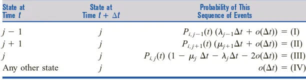
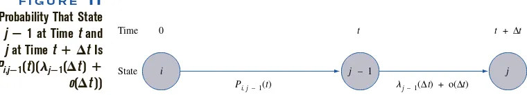
are four ways for the state at time t tto be j. For j 1, the four ways are shown in Table 3. For j1, the probability that the state of the system will be j1 at time tand jat time t tis (see Figure 11)
Pi,j1(t)(lj1to(t))
Similar arguments yield (II) and (III). (IV) follows, because if the system is in a state other than j, j1, or j1 at time t, then to end up in state jat time t t, more than one event (birth or death) must occur between tand t t. By law 3, this has probabil-ity o(t). Thus,
Pij(t t) (I) (II) (III) (IV)
After regrouping terms in this equation, we obtain
Pij(t t) Pij(t)
t(lj1Pi,j1(t) mj1Pi,j1(t) Pij(t)mjPij(t)lj) (10) o(t)(Pi,j1(t) Pi,j1(t) 1 2Pij(t))
Since the underlined term may be written as o(t), we rewrite (10) as
Pij(t t) Pij(t) t(lj1Pi,j1(t) mj1Pi,j1(t) Pij(t)mj Pij(t)lj) o(t)
Dividing both sides of this equation by tand letting tapproach zero, we see that for all iand j1,
Pij(t) lj1Pi,j1(t) mj1Pi,j1(t) Pij(t)mj Pij(t)lj (10ⴕ)
Since for j0, Pi,j1(t) 0 and mj0, we obtain, for j0,
Pi,0(t) m1Pi,1(t) l0Pi,0(t)
This is an infinite system of differential equations. (A differential equation is simply an equation in which a derivative appears.) In theory, these equations may be solved for the Pij(t). In reality, however, this system of equations is usually extremely difficult to solve.
All is not lost, however. We can use (10) to obtain the steady-state probabilities pj(j
0, 1, 2, . . .). As with Markov chains, we define the steady-state probability pjto be
lim
t→∞
Pij(t)
Then for large t and any initial state i, Pij(t) will not change very much and may be
thought of as a constant. Thus, in the steady state (tlarge), Pij(t) 0. In the steady state,
T A B L E 3
Computations of Probability That State at Time tⴙtIs j
State at State at Probability of This
Time t Time tⴙt Sequence of Events
j1 j Pi, j1(t) (lj1to(t)) (I)
j1 j Pi, j1(t) (mj1to(t)) (II)
j j Pi, j(t) (1 mjt ljt2o(t)) (III)
also, Pi,j1(t) pj1, Pi,j1(t) pj1, and Pij(t) pjwill all hold. Substituting these
relations into (10), we obtain, for j 1,
lj1pj1mj1pj1pjmjpjlj0 (10ⴖ) lj1pj1mj1pj1pj(ljmj) (j1, 2, . . .)
For j0, we obtain
m1p1p0l0
Equations (10) are an infinite system of linearequations that can be easily solved for the
pj’s. Before discussing how to solve (10), we give an intuitive derivation of (10), based
on the following observation: At any time t that we observe a birth–death process, it must be true that for each state j, the number of times we have entered state j differs by at most 1 from the number of times we have left state j.
Suppose that by time t, we have entered state 6 three times. Then one of the cases in Table 4 must have occurred. For example, if Case 2 occurs, we begin in state 6 and end up in some other state. Since we have observed three transitions into state 6 by time t, the following events (among others) must have occurred:
Start in state 6 Enter state 6 (second time) Leave state 6 (first time) Leave state 6 (third time) Enter state 6 (first time) Enter state 6 (third time) Leave state 6 (second time) Leave state 6 (fourth time)
Hence, if Case 2 occurs, then by time t, we must have left state 6 four times.
This observation suggests that for large t and for j 0, 1, 2, . . . (and for any initial conditions), it will be true that
(11)
Assuming the system has settled down into the steady state, we know that the system spends a fraction pjof its time in state j. We can now use (11) to determine the
steady-state probabilities pj. For j1, we can only leave state jby going to state j1 or state
j1, so for j1, we obtain
pj(lj mj) (12)
Since for j1 we can only enter state jfrom state j1 or state j1,
pj1lj1pj1mj1 (13)
Substituting (12) and (13) into (11) yields
pj1lj1pj1mj1pj(ljmj) (j 1, 2, . . .) (14)
Expected no. of entrances into state j
Expected no. of departures from state j
Expected no. of entrances into state j
Expected no. of departures from state j
j – 1 State
Time 0 t
Pi, j – 1(t) j – 1(∆t) + o(∆t)
t + ∆t
i j
F I G U R E 11
Probability That State Is jⴚ1 at Time tand
jat Time tⴙ ⌬tIs
Pi,jⴚ1(t)(ljⴚ1(⌬t) ⴙ
For j0, we know that m0p10, so we also have
p1m1p0l0 (14ⴕ)
Equations (14) and (14) are often called the flow balance equations,or conservation of flow equations,for a birth–death process. Note that (14) expresses the fact that in the steady state, the rate at which transitions occur into any state imust equal the rate at which transitions occur out of state i. If (14) did not hold for all states, then probability would “pile up” at some state, and a steady state would not exist.
Writing out the equations for (14) and (14), we obtain the flow balance equations for a birth–death process:
(j0) p0l0p1m1
(j1) (l1m1)p1l0p0m2p2
(j2) (l2m2)p2l1p1m3p3 (15)
(jth equation) (ljmj)pj lj1pj1mj1pj1
Solution of Birth–Death Flow Balance Equations
To solve (15), we begin by expressing all the pj’s in terms of p0. From the (j0)
equa-tion, we obtain
p1 p
m 0l
1 0
Substituting this result into the (j1) equation yields
l0p0m2p2
(l1 m
m
1 1)p0l0
m2p2 p0(
m l0
1 l1)
Thus,
p2 p0
m
(l
1m 0l
2 1)
We could now use the (j 3) equation to solve for p3in terms of p0and so on. If we
define
cj
l
m 0l
1m 1
2
l
m j
j 1
T A B L E 4
Relation between Number of Transitions into and out of a State by Time t
Number of Transitions Initial State State of Time t Out of State 6 by Time t
Case 1: state 6 State 6 3
Case 2: state 6 Any state except 6 4
Case 3: any state
except state 6 State 6 2
Case 4: any state
then it can be shown that
pjp0cj (16)
(See Problem 1 at the end of this section.) Since at any given time, we must be in some state, the steady-state probabilities must sum to 1:
冱
j∞
j0
pj1 (17)
Substituting (16) into (17) yields
p0
冢
1冱
j∞j1
cj
冣
1 (18)If 冱jj∞1 cjis finite, we can use (18) to solve for p0:
p0 (19)
Then (16) can be used to determine p1, p2, . . . . It can be shown that if 冱jj∞1 cjis
infi-nite, then no steady-state distribution exists. The most common reason for a steady-state failing to exist is that the arrival rate is at least as large as the maximum rate at which customers can be served.
Using a Spreadsheet to Compute Steady-State Probabilities
The following example illustrates how a spreadsheet can be used to compute steady-state probabilities for a birth–death process.
E X A M P L E 2
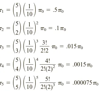
Indiana Bell customer service representatives receive an average of 1,700 calls per hour. The time between calls follows an exponential distribution. A customer service represen-tative can handle an average of 30 calls per hour. The time required to handle a call is also exponentially distributed. Indiana Bell can put up to 25 people on hold. If 25 people are on hold, a call is lost to the system. Indiana Bell has 75 service representatives.
1 What fraction of the time are all operators busy?
2 What fraction of all calls are lost to the system?
Solution In Figure 12 (file Bell.xls), we set up a spreadsheet to compute the steady-state probabil-ities for this birth–death process. We let the state iat any time equal the number of callers whose calls are being processed or are on hold. We have that for i 0, 1, 2, . . . , 99,
li1,700. The fact that any calls received when 75 25 100 calls are in the system are lost to the system implies that l1000. Then no state i100 can occur (why?). We
have u00 and for i1, 2, . . . , 75, mi30i. For i75, mi30(75) 2,250.
To answer parts (1) and (2), we need to compute the steady-state probabilities pi
fraction of the time the state is i. In cells A4:A104, we enter the possible states of the sys-tem (0–100). To do this, enter 0 in cell A4 and 1 in A5. Then select the range A4:A5 and drag the cursor to A6:A104. In B4, type the arrival rate of 1,700 and just drag the cursor
Indiana Bell
1
1
冱
j∞j1 cj
1
INDIANA BELL EXAMPLE 0 .012759326
STATE LAMBDA MU CJ PROB
0 1700 0 1 2.451E-25
1 1700 30 56.6666667 1.3889E-23
2 1700 60 1605.55556 3.9352E-22
3 1700 90 30327.1605 7.4332E-21
4 1700 120 429634.774 1.053E-19
5 1700 150 4869194.1 1.1934E-18
6 1700 180 45986833.2 1.1271E-17
7 1700 210 372274364 9.1244E-17
8 1700 240 2636943411 6.4631E-16 9 1700 270 1.6603E+10 4.0694E-15 10 1700 300 9.4084E+10 2.306E-14 11 1700 330 4.8467E+11 1.1879E-13 12 1700 360 2.2887E+12 5.6097E-13 13 1700 390 9.9765E+12 2.4452E-12 14 1700 420 4.0381E+13 9.8974E-12 15 1700 450 1.5255E+14 3.739E-11 16 1700 480 5.4029E+14 1.3242E-10 17 1700 510 1.801E+15 4.4141E-10 18 1700 540 5.6697E+15 1.3896E-09 19 1700 570 1.691E+16 4.1445E-09 20 1700 600 4.791E+16 1.1743E-08 21 1700 630 1.2928E+17 3.1687E-08
22 1700 660 3.33E+17 8.1618E-08
23 1700 690 8.2043E+17 2.0109E-07 24 1700 720 1.9371E+18 4.7479E-07 25 1700 750 4.3908E+18 1.0762E-06 26 1700 780 9.5697E+18 2.3455E-06 27 1700 810 2.0085E+19 4.9227E-06 28 1700 840 4.0648E+19 9.9627E-06 29 1700 870 7.9426E+19 1.9467E-05 30 1700 900 1.5003E+20 3.6772E-05 31 1700 930 2.7424E+20 6.7217E-05 32 1700 960 4.8564E+20 0.00011903 33 1700 990 8.3393E+20 0.00020439 34 1700 1020 1.3899E+21 0.00034066 35 1700 1050 2.2503E+21 0.00055154 36 1700 1080 3.5421E+21 0.00086817 37 1700 1110 5.4248E+21 0.00132962 38 1700 1140 8.0897E+21 0.00198277 39 1700 1170 1.1754E+22 0.00288095 40 1700 1200 1.6652E+22 0.00408134 41 1700 1230 2.3015E+22 0.00564088 42 1700 1260 3.1052E+22 0.00761072 43 1700 1290 4.0921E+22 0.01002963 44 1700 1320 5.2701E+22 0.01291694 45 1700 1350 6.6364E+22 0.01626578 46 1700 1380 8.1753E+22 0.02003755 47 1700 1410 9.8567E+22 0.02415875 48 1700 1440 1.1636E+23 0.02852075 49 1700 1470 1.3457E+23 0.03298318 50 1700 1500 1.5251E+23 0.03738094 51 1700 1530 1.6946E+23 0.04153437 52 1700 1560 1.8467E+23 0.04526182 53 1700 1590 1.9744E+23 0.04839314 54 1700 1620 2.0719E+23 0.05078292 55 1700 1650 2.1347E+23 0.0523218 56 1700 1680 2.1601E+23 0.05294468
E F
F I G U R E 12
down to B5:B104 to create the arrival rates for all states. To create the service rates, en-ter 0 in cell C4. Then enen-ter 30 in C5 and 60 in cell C6. Then select the range C5:C6 and drag the cursor down to C79. This creates the service rates for states 0–75. In C80, enter 2,250 and drag that result down to C81:C104. This creates the service rate (2,250) for states 76–100. In the cell range D4:D104, we calculate the cj’s that are needed to
com-pute the steady-state probabilities. To begin, we enter a 1 in D4. Since c1l0/m1, we
en-ter B4/C5 in cell D5. Since c2c1l1/m2, we enter D5*B5/C6 into D6. Copying from
D6 to D7:D104 now generates the rest of the cj’s. In E4, we compute p0 by entering
SUM(D$4:D$104). In E5, we compute p1 by entering D5*E$4. Copying from the
range E5 to the range E5:E104 generates the rest of the steady-state probabilities. We can now answer questions (1) and (2).
1 We seek p75 p76 p100. To obtain this, we enter the command
SUM(E79:E104) in cell F2 and obtain .013.
2 An arriving call is turned away if the state equals 100. A fraction p100.0000028 of
all arrivals will be turned away. Thus, the phone company is providing very good service!
In Sections 20.4–20.6 and 20.9–20.10, we apply the theory of birth–death processes to determine the steady-state probability distributions for a variety of queuing systems. Then we use the steady-state probability distributions to determine other quantities of interest (such as expected waiting time and expected number of customers in the system).
Birth–death models have been used to model phenomena other than queuing systems. For example, the number of firms in an industry can be modeled as a birth–death process: The state of the industry at any given time is the number of firms that are in business; a birth corresponds to a firm entering the industry; and a death corresponds to a firm go-ing out of business.
P R O B L E M S
Group A
1 Show that the values of the pj’s given in (16) do indeed satisfy the flow balance equations (14) and (14).
2 My home uses two light bulbs. On average, a light bulb lasts for 22 days (exponentially distributed). When a light bulb burns out, it takes an average of 2 days (exponentially distributed) before I replace the bulb.
a Formulate a three-state birth–death model of this situation.
b Determine the fraction of the time that both light bulbs are working.
c Determine the fraction of the time that no light bulbs are working.
Group B
3 You are doing an industry analysis of the Bloomington pizza industry. The rate (per year) at which pizza restaurants enter the industry is given by p, where pprice of a pizza in dollars. The price of a pizza is assumed to be max(0, 16 .5F), where F number of pizza restaurants in Bloomington. During a given year, the probability that a pizza restaurant fails is 1/(10 p). Create a birth–death model of this situation.
a In the steady state, estimate the average number of pizza restaurants in Bloomington.
b What fraction of the time will there be more than 20 pizza restaurants in Bloomington?
20.4
The
M
/
M
/1/
GD
/
∞
/
∞
Queuing System
and the Queuing Formula
L
ⴝ
l
W
We now use the birth–death methodology explained in the previous section to analyze the properties of the M/M/1/GD/∞/∞queuing system. Recall that the M/M/1/GD/∞/∞ queuing system has exponential interarrival times (we assume that the arrival rate per unit time is l) and a single server with exponential service times (we assume that each customer’s service time is exponential with rate m). In Section 20.3, we showed that an M/M/1/GD/∞/∞queuing system may be modeled as a birth–death process with the following parameters:
ljl (j0, 1, 2, . . .)
m00 (20)
Derivation of Steady-State Probabilities
We can use Equations (15)–(19) to solve for pj, the steady-state probability that j cus-tomers will be present. Substituting (20) into (16) yields
p1 l
m p0
, p2
l m 2
p 2 0
, . . . , pj l m
jp
j 0
(21)
We define r ml. For reasons that will become apparent later, we call rthe traffic
in-tensityof the queuing system. Substituting (21) into (17) yields
p0(1 rr2 ) 1 (22)
We now assume that 0 r 1. Then we evaluate the sum S 1 rr2 as follows: Multiplying Sby ryields rSr r2 r3 . Then SrS 1, and
S
1
1
r (23)
Substituting (23) into (22) yields
p01 r (0 r1) (24)
Substituting (24) into (21) yields
pjrj(1 r) (0 r1) (25)
If r1, however, the infinite sum in (22) “blows up” (try r1, for example, and you get 1 1 1 ). Thus, if r1, no steady-state distribution exists. Since r ml, we see that if lm(that is, the arrival rate is at least as large as the service rate), then no steady-state distribution exists.
If r1, it is easy to see why no steady-state distribution can exist. Suppose l 6 customers per hour and m 4 customers per hour. Even if the server were working all the time, she could only serve an average of 4 people per hour. Thus, the average num-ber of customers in the system would grow by at least 6 4 2 customers per hour. This means that after a long time, the number of customers present would “blow up,” and no steady-state distribution could exist. If r1, the nonexistence of a steady state is not quite so obvious, but our analysis does indicate that no steady state exists.
Derivation of L
Throughout the rest of this section, we assume that r 1, ensuring that a steady-state probability distribution, as given in (25), does exist. We now use the steady-state proba-bility distribution in (25) to determine several quantities of interest. For example, assum-ing that the steady state has been reached, the average number of customers present in the queuing system (call it L) is given by
L
冱
j∞
j0
jpj
冱
j∞j0
jrj(1 r)
(1 r)
冱
j∞
j0 jrj
Defining
S
冱
j∞
j0
we see that rS r2 2r33r4 . Subtracting yields
In some circumstances, we are interested in the expected number of people waiting in line (or in the queue). We denote this number by Lq. Note that if 0 or 1 customer is present in
the system, then nobody is waiting in line, but if jpeople are present (j1), there will be j1 people waiting in line. Thus, if we are in the steady state,
Since every customer who is present is either in line or in service, it follows that for any queuing system (not just an M/M/1/GD/∞/∞system), LLsLq. Thus, using our
for-Often we are interested in the amount of time that a typical customer spends in a queu-ing system. We define Was the expected time a customer spends in the queuing system, including time in line plus time in service, and Wqas the expected time a customer spends
waiting in line. Both Wand Wqare computed under the assumption that the steady state
Wq may be easily computed from L and Lq. We first define (for any queuing system or
any subset of a queuing system) the following quantities:
l average number of arrivals enteringthe system per unit time L average number of customers present in the queuing system Lq average number of customers waiting in line
Ls average number of customers in service
W average time a customer spends in the system Wq average time a customer spends in line
Ws average time a customer spends in service
In these definitions, all averages are steady-state averages. For most queuing systems, Lit-tle’s queuing formula may be summarized as in Theorem 3.
T H E O R E M 3
For anyqueuing system in which a steady-state distribution exists, the following re-lations hold:
L lW (28)
Lq lWq (29)
Ls lWs (30)
Before using these important results, we present an intuitive justification of (28). First note that both sides of (28) have the same units (we assume the unit of time is hours). This follows, because L is expressed in terms of number of customers, lis expressed in terms of customers per hour, and W is expressed in hours. Thus, lW has the same units (customers) as L. For a rigorous proof of Little’s theorem, see Ross (1970). We content ourselves with the following heuristic discussion.
Consider a queuing system in which customers are served on a first come, first served basis. An arbitrary arrival enters the system (assume that the steady state has been reached). This customer stays in the system until he completes service, and upon his de-parture, there will be (on the average) L customers present in the system. But when this customer leaves, who will be left in the system? Only those customers who arrive during the time the initial customer spends in the system. Since the initial customer spends an average of Whours in the system, an average of lWcustomers will arrive during his stay in the system. Hence, LlW. The “real” proof of LlWis virtually independent of the number of servers, the interarrival time distribution, the service discipline, and the ser-vice time distribution. Thus, as long as a steady state exists, we may apply Equations (28)–(30) to any queuing system.
To illustrate the use of (28) and (29), we determine Wand Wqfor an M/M/1/GD/∞/∞
queuing system. From (26),
L
1
r
r
Then (28) yields
W L
l l(1
r
r) m
1
From (27), we obtain
Lq
m(m l
2
l) and (29) implies
Wq
L
l q
m(m
l
l) (32)
Notice that (as expected) as rapproaches 1, both Wand Wqbecome very large. For rnear
zero, Wqapproaches zero, but for small r, Wapproaches m1, the mean service time.
The following three examples show applications of the formulas we have developed.
E X A M P L E 3
An average of 10 cars per hour arrive at a single-server drive-in teller. Assume that the average service time for each customer is 4 minutes, and both interarrival times and ser-vice times are exponential. Answer the following questions:
1 What is the probability that the teller is idle?
2 What is the average number of cars waiting in line for the teller? (A car that is being served is not considered to be waiting in line.)
3 What is the average amount of time a drive-in customer spends in the bank parking lot (including time in service)?
4 On the average, how many customers per hour will be served by the teller?
Solution By assumption, we are dealing with an M/M/1/GD/∞/∞queuing system for which l
10 cars per hour and m15 cars per hour. Thus, r 1105 23.
1 From (24), p01 r1 23 13. Thus, the teller will be idle an average of
one-third of the time.
2 We seek Lq. From (27),
Lq
1
r
2
r
4
3 customers
3 We seek W. From (28), W Ll. Then from (26).
L
1
r
r
2 customers
Thus, W 120 15 hour 12 minutes (Wwill have the same units as l).
4 If the teller were always busy, he would serve an average of m 15 customers per hour. From part (1), we know that the teller is only busy two-thirds of the time. Thus, dur-ing each hour, the teller will serve an average of (23)(15) 10 customers. This must be the case, because in the steady state, 10 customers are arriving each hour, so each hour, 10 customers must leave the system.
E X A M P L E 4
Suppose that all car owners fill up when their tanks are exactly half full.†At the present time, an average of 7.5 customers per hour arrive at a single-pump gas station. It takes an
Service Station
2 3
(23)2
1 23
Drive-in Banking