http://doi.org/10.17576/jsm-2022-5104-22
The Occurred Error in Microdosimetry Calculations while Using Water Instead of the Body Organs in Proton Therapy and a New Formula for an Estimate of the
Statistical Uncertainty of Microdosimetric Quantities
(Ralat Berlaku dalam Pengiraan Mikrodosimetri semasa Menggunakan Air Bukan Organ Badan dalam Terapi Proton dan Formula Baharu untuk Anggaran Ketidakpastian Statistik Kuantiti Mikrodosimetrik)
SOMAYEH JAHANFAR& HOSSEIN TAVAKOLI-ANBARAN*
Faculty of Physics and Nuclear Engineering, Shahrood University of Technology, Shahrood, Iran Received: 4 June 2021/Accepted: 26 August 2021
ABSTRACT
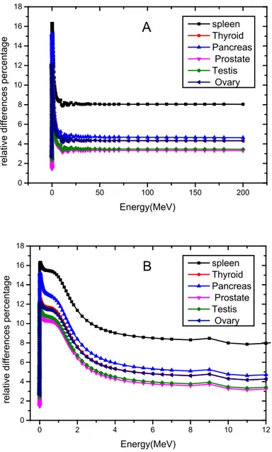
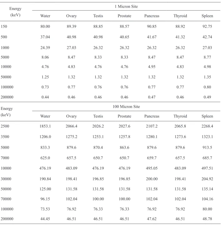
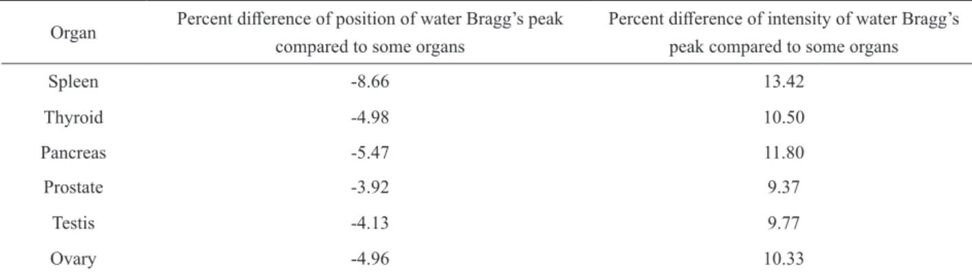
In many experimental and simulation researches, water phantom is used instead of most body organs. Therefore, in this study, we replaced the water phantom instead of some organs to calculate its effect on the proton stopping-power, and range and the consequence of deposited energy and microdosimetric spectra in small sites. Some organs such as the spleen, thyroid, pancreas, prostate, testis, and ovaries are considered. We calculated the proton stopping-power in these organs using the SRIM code. Then using these results, we wrote a program in the programming language of Fortran and computed the proton range and deposited energy in two sites of 1 and 100 micron. Also, using the Geant4-10-4 code, we simulated these sites and obtained microdosimetric spectra of protons at 1 and 5MeV energies. In order to compare different states, the frequency-mean lineal energy, dose-mean lineal energy, these statistical uncertainties and absorb dose in each case were calculated and reported. Also, we estimated the statistical uncertainty of quantities with a new formula. We observed that using water instead of the organs causes a significant error in the calculations of the range and the maximum relative difference percentage of 18% and 22% in deposited energy in 1 and 100 micron sites, respectively. These differences depend on the energy of the incident proton, organ, and size site. Also, this replacement changes microdosimetric spectra, the location, and intensity of the Bragg’s peak. The percent difference of location and intensity of the Bragg’s peak for water instead of the spleen is -8.66 and 13.42%, respectively. Therefore, using water instead of the body organs in microdosimetry calculations is not recommended.
Keywords: Body organs and water; microdosimetry; proton range and stopping power; proton therapy; statistical uncertainty
ABSTRAK
Dalam banyak penyelidikan uji kaji dan simulasi, fantom air digunakan sebagai ganti kebanyakan organ tubuh. Oleh itu, dalam kajian ini, kami menggantikan fantom air dan bukannya beberapa organ untuk menghitung kesannya pada daya berhenti proton dan julat serta akibat daripada tenaga dan spektrum mikrodosimetri yang tersimpan di lokasi kecil. Beberapa organ seperti limpa, tiroid, pankreas, prostat, testis dan ovari dipertimbangkan. Kami menghitung daya berhenti proton pada organ-organ ini menggunakan kod SRIM. Kemudian, menggunakan hasil ini, kami menulis sebuah program dalam bahasa pengaturcaraan Fortran dan menghitung julat proton dan menyimpan tenaga di dua lokasi antara 1 dan 100 mikron. Juga, menggunakan kod Geant4-10-4, kami mensimulasi lokasi ini dan memperoleh spektrum mikrodosimetri proton pada tenaga 1 dan 5MeV. Untuk membandingkan keadaan yang berlainan, tenaga linear frekuensi-min, tenaga garis lurus-dosis, ketidakpastian statistik ini dan penyerap dos dalam setiap kes dihitung dan dilaporkan. Kami juga menganggarkan ketidaktentuan statistik kuantiti dengan formula baru. Kami memerhatikan bahawa penggunaan air sebagai ganti organ telah menyebabkan ralat yang ketara dalam pengiraan julat dan peratusan perbezaan relatif maksimum 18% dan 22% tenaga yang tersimpan masing-masing di lokasi 1 dan 100 mikron. Perbezaan ini bergantung pada tenaga proton, organ dan ukuran saiz lokasi. Juga, penggantian ini mengubah spektrum mikrodosimetri, lokasi dan keamatan puncak Bragg. Perbezaan peratus lokasi dan keamatan puncak Bragg untuk air dan bukannya limpa masing-masing adalah -8.66 dan 13.42%. Oleh itu, penggunaan air bukan organ tubuh dalam pengiraan mikrodosimetri tidak digalakkan.
Kata kunci: Julat proton dan daya berhenti; ketidaktentuan statistik; mikrodosimetri; organ badan dan air; terapi proton
INTRODUCTION
In radiation therapy, cancer organs are exposed to ionizing radiation to prevent their growth and proliferation. To treat various cancers such as cancer of the brain, breast, lung, prostate, stomach, and other benign tumors, radiation therapy is used (Shahrabi et al.
2015). The beam emits energy along the path it travels, and so the stopping power is obtained from (1):
(1) In this regard, L(s) are the stop numbers and include correction factors with different powers for high-velocity particles,β υ= / c, κ =4πe N m c4 / e 2 and Z1 is the charge of the incident particle and z2 is the atomic number of matter (Ziegler 1999; Ziegler et al. 2008). Due to the fact that the body organs are composed of different elements, so the calculation of the stopping power in the organ must include the formula of composition which is as follows:
(2) In the above relation, ρ is the density and wi is the weight fraction of each element (Tsoulfanidis 2015).
And the range is obtained by (3):
(3) Proton therapy (direct) and neutron therapy (backscattering of the nucleus of hydrogen atoms) require accurate information on the mechanism of energy transfer of protons to the organ (Khan et al. 2014).
Therefore, according to the different sensitivities of the organs to radiation in order to calculate the deposited energy in the organ (Rasouli et al. 2017), gathering accurate information about the stopping power and consequently the range of the beam in different organs is important. On the other hand, due to the easy access and homogeneity of water and the proximity of water absorption properties to soft tissues (Liu et al. 2003) as well as the proximity of water density to body organs, this substance has become an important substance in biology and in most researches, the water is used instead of body organs (Akiyama et al. 1992; Blosser et al. 1964;
Thomas et al. 1979; Toburen et al. 1977).
According to Mitchell et al. (1945), the chemical composition of different organs is different and therefore
the share of water in them is also different. In adults, for example, the brain, heart, pancreas, lungs, kidneys, spleen, liver, and skin are made up of 73.33, 73.69, 73.08, 83.74, 79.47, 78.69, 71.46, and 64.68% water, respectively, and even the bones are made up of 31.81%
water (Mitchell et al. 1945). Also, because the human body is made up of different organs with different densities, using water instead of the real organ can be one of the sources of error (Ahmadi & Tavakoli-Anbaran 2015) to determine the stopping power and range and consequently deposited energy in tissue accurately.
In the following, it is necessary to briefly state the quantities used in microdosimetry. Lineal energy (
y ε1
= ι ) is expressed as 𝑘𝑘𝑘𝑘𝑘𝑘𝜇𝜇𝜇𝜇 and ι is the mean chord length, and ε1 is the energy imparted in the target in a single event (Cornelius et al. 2002; Lindborg et al. 2017;
Northum et al. 2012; Reniers et al. 2004; Rosenfeld et al. 2000; Tsuda et al. 2010). Cauchy’s theorem for a convex object states: The mean chord length is4 /V S, where V and S are the volume and surface of the site, respectively. Lineal energy distribution f(y) is the probability density of lineal energy and f(y)dy is the probability of lineal energy being in the event of an interval of
[
y y dy, +]
(Bolst et al. 2017; Rossi et al. 2011).The dose probability density is defined as follow:
(4)
In the above relation, yF is known as the frequency- mean lineal energy, as follows (Burigo et al. 2013;
ICRU 1983; Kliauga & Rossi 1982; Rosenfeld 2016).
(5)
Also, the dose-mean lineal energy defines as follows (Chattaraj et al. 2018; Pan et al. 2015).
(6)
The statistical uncertainty estimated in yF using the error propagation formula is given as:
(7)
2 2
2 1 0 1 1 1 2
2 ( ( ) ( ) ( ) ..., )
S z Z L Z L Z L
= + + +
( )compound i( )
i i
dE w dE
dx dx
− =
−
, ( ) ( )
( )
dE dE
R f E
f E dx
=
− =2 2
2 1 0 1 1 1 2
2 ( ( ) ( ) ( ) ..., )
S z Z L Z L Z L
= + + +
( )compound i( )
i i
dE w dE
dx dx
− =
−
, ( ) ( )
( )
dE dE
R f E
f E dx
=
− =2 2
2 1 0 1 1 1 2
2 ( ( ) ( ) ( ) ..., )
S z Z L Z L Z L
= + + +
( )compound i( )
i i
dE w dE
dx dx
− =
−
, ( ) ( )
( )
dE dE
R f E
f E dx
=
− =( ) ( )
F
d y y f y
= y
0 F ( )
y =
yf y dy2 0 0
0
( ) ( )
( )
D
y f y dy y yd y dy
yf y dy
= =
𝜎𝜎𝑦𝑦̅𝑦𝑦̅𝐹𝐹
𝐹𝐹
= √
(∑ 𝑦𝑦∑ 𝑦𝑦𝑖𝑖 𝑖𝑖2𝑓𝑓(𝑦𝑦𝑖𝑖)𝑖𝑖𝑓𝑓(𝑦𝑦𝑖𝑖)
𝑖𝑖 )2
+
(∑ 𝑓𝑓(𝑦𝑦∑ 𝑓𝑓(𝑦𝑦𝑖𝑖 𝑖𝑖)𝑖𝑖)
𝑖𝑖 )2
( ) ( )
F
d y y f y
=y
0 F ( )
y =
yf y dy2 0 0
0
( ) ( )
( )
D
y f y dy y yd y dy
yf y dy
= =
𝜎𝜎𝑦𝑦̅𝑦𝑦̅𝐹𝐹
𝐹𝐹
= √
(∑ 𝑦𝑦∑ 𝑦𝑦𝑖𝑖 𝑖𝑖2𝑓𝑓(𝑦𝑦𝑖𝑖)𝑖𝑖𝑓𝑓(𝑦𝑦𝑖𝑖)
𝑖𝑖 )2
+
(∑ 𝑓𝑓(𝑦𝑦∑ 𝑓𝑓(𝑦𝑦𝑖𝑖 𝑖𝑖)𝑖𝑖)
𝑖𝑖 )2
( ) ( )
F
d y y f y
=y
0 F ( )
y =
yf y dy2 0 0
0
( ) ( )
( )
D
y f y dy y yd y dy
yf y dy
= =
𝜎𝜎𝑦𝑦̅𝑦𝑦̅𝐹𝐹
𝐹𝐹
= √
(∑ 𝑦𝑦∑ 𝑦𝑦𝑖𝑖 𝑖𝑖2𝑓𝑓(𝑦𝑦𝑖𝑖)𝑖𝑖𝑓𝑓(𝑦𝑦𝑖𝑖)
𝑖𝑖 )2
+
(∑ 𝑓𝑓(𝑦𝑦∑ 𝑓𝑓(𝑦𝑦𝑖𝑖 𝑖𝑖)𝑖𝑖)
𝑖𝑖 )2
( ) ( )
F
d y y f y
= y
0 F ( )
y =
yf y dy2 0 0
0
( ) ( )
( )
D
y f y dy y yd y dy
yf y dy
= =
𝜎𝜎𝑦𝑦̅𝑦𝑦̅𝐹𝐹
𝐹𝐹
= √
(∑ 𝑦𝑦∑ 𝑦𝑦𝑖𝑖 𝑖𝑖2𝑓𝑓(𝑦𝑦𝑖𝑖)𝑖𝑖𝑓𝑓(𝑦𝑦𝑖𝑖)
𝑖𝑖 )2
+
(∑ 𝑓𝑓(𝑦𝑦∑ 𝑓𝑓(𝑦𝑦𝑖𝑖 𝑖𝑖)𝑖𝑖)
𝑖𝑖 )2 ,
A similar expression results for
y
D (Aslam et al.2003). In this article, we examined what errors and changes that occur in the calculations of stopping power and range and consequently, the deposited energy in the site and also in microdosimetric spectra through placing water instead of some organs in proton therapy.
We also estimated the statistical uncertainty of quantities with a new formula and compared these quantities in different states with two formulas.
MATERIALS AND METHODS
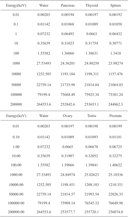
In this article, using the SRIM code, we obtained the proton stopping power in liquid water and six organs of
the body’s important organs, including the spleen, thyroid, pancreas, prostate, testicles, and ovaries, the elements of each are stated in Table 1.
Since the stopping power is a complicated expression, a numerical integration is required. In order to calculate the range and deposited energy, we wrote a program in the Fortran programming language using formula 3, the proton stopping power data of the SRIM code for water and the mentioned organs and dimension site. Formula 3 is divided into N segments of ∆Ei,
( / )
N i
i i
R E
dE dx
= ∆
∑
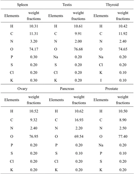
− , where (dE dx/ )i is the stopping power calculated for the kinetic energy of the particle at the beginning of the segment ∆Ei.TABLE 1. Elements and weight fractions of some organs of the body (Ziegler et al. 2008)
Spleen Testis Thyroid
Elements weight
fractions Elements weight
fractions Elements weight fractions
H 10.31 H 10.61 H 10.42
C 11.31 C 9.91 C 11.92
N 3.20 N 2.00 N 2.40
O 74.17 O 76.68 O 74.65
P 0.30 Na 0.20 Na 0.20
S 0.20 S 0.20 Cl 0.20
Cl 0.20 Cl 0.20 K 0.10
K 0.30 K 0.20 I 0.10
Ovary Pancreas Prostate
Elements weight
fractions Elements weight
fractions Elements weight fractions
H 10.52 H 10.62 H 10.50
C 9.32 C 16.93 C 8.90
N 2.40 N 2.20 N 2.50
O 76.95 O 69.54 O 77.40
P 0.20 P 0.20 Na 0.20
S 0.20 S 0.10 P 0.10
Cl 0.20 Cl 0.20 S 0.20
K 0.20 K 0.20 K 0.20
Then to verify our program, we wrote an input file using the MCNPX code for the proton point source at 200 MeV. We placed a sphere of the water in front of the source. In this code, we obtained the stopping power of the proton using the print card and output table 85.
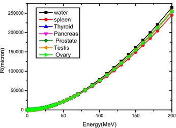
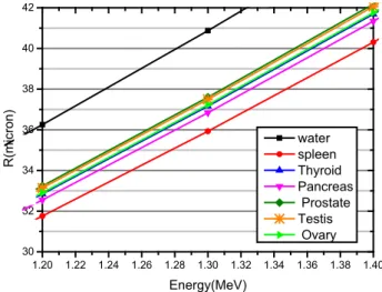
We compared results of the proton range of our own program in Fortran with the results obtained from the MCNPX code, and after ensuring the performance of our program, we calculated the range and deposited energy in the 1 and 100 micron sites using this program. We also calculated the relative difference of proton range in water and each of these organs. In addition, we calculated and plotted the Bragg peak curve in terms of different thicknesses of water and organs. In the following, using the Geant4-10-4 code, we simulated sites of 1 and 100 microns of water and body organs for the proton with energies of 1 and 5 MeV and 0 micron cut-off.
Micron sites with water materials and organs were simulated in the detector-construction class and physics were also simulated using reference physics lists of QGSP_BIC_HP in the physics-list class. We considered the 300 logarithmic intervals of lineal energy from 0.001 to 1000𝑘𝑘𝑘𝑘𝑘𝑘
𝜇𝜇𝜇𝜇 and 50 logarithmic intervals per decade, the probability density of lineal energy or f(y) in each interval is calculated so that finally we calculated the microdosimetric spectra using formulas 4 and 5.
We also used formulas 5, 6, and 7 to calculate other microdosimetric quantities and statistical uncertainty of these quantities. It is worth noting that the information required for Monte Carlo simulations according to Sechopoulos et al. (2018) is stated.
We also estimated the statistical uncertainty of quantities with a new formula. Assume that in arbitrary function f(x), the quantity x is examined. In the problems studied by the Monte Carlo method, f (xi) is counts or frequency of quantity x in the bin “i”, N is the total number of bins, f (xi) =
, 𝑓𝑓(𝑥𝑥𝑖𝑖) = 𝑛𝑛𝑖𝑖/∆𝑦𝑦𝑖𝑖, standard deviation of Poisson distribution function 𝜎𝜎𝑓𝑓(𝑥𝑥𝑖𝑖)= √𝑛𝑛𝑖𝑖/∆𝑦𝑦𝑖𝑖 and 𝐺𝐺(𝑥𝑥) = 𝑥𝑥𝑏𝑏𝑓𝑓(𝑥𝑥). If the lineal energy widths of the intervals are the same𝜎𝜎𝑓𝑓(𝑥𝑥𝑖𝑖)= √𝑛𝑛𝑖𝑖/∆𝑦𝑦.
, standard deviation of Poisson distribution function
, 𝑓𝑓(𝑥𝑥𝑖𝑖) = 𝑛𝑛𝑖𝑖/∆𝑦𝑦𝑖𝑖, standard deviation of Poisson distribution function 𝜎𝜎𝑓𝑓(𝑥𝑥𝑖𝑖)= √𝑛𝑛𝑖𝑖/∆𝑦𝑦𝑖𝑖 and 𝐺𝐺(𝑥𝑥) = 𝑥𝑥𝑏𝑏𝑓𝑓(𝑥𝑥). If the lineal energy widths of the intervals are the same𝜎𝜎𝑓𝑓(𝑥𝑥𝑖𝑖)= √𝑛𝑛𝑖𝑖/∆𝑦𝑦.
and G(x)
= xb f (x). If the lineal energy widths of the intervals are the same
, 𝑓𝑓(𝑥𝑥𝑖𝑖) = 𝑛𝑛𝑖𝑖/∆𝑦𝑦𝑖𝑖, standard deviation of Poisson distribution function 𝜎𝜎𝑓𝑓(𝑥𝑥𝑖𝑖)= √𝑛𝑛𝑖𝑖/∆𝑦𝑦𝑖𝑖 and 𝐺𝐺(𝑥𝑥) = 𝑥𝑥𝑏𝑏𝑓𝑓(𝑥𝑥). If the lineal energy widths of the intervals are the same𝜎𝜎𝑓𝑓(𝑥𝑥𝑖𝑖)= √𝑛𝑛𝑖𝑖/∆𝑦𝑦.
. The average or the expectation value of x, is defined by the equation:
(8)
we have from the error propagation formula:
(9)
We will have:
(10)
We rewrite (10) by f (xi ) = ni/∆y:
(11)
By replacing xi to yi we have:
(12)
If b = 0 then
( ) 1 𝜎𝜎𝑥𝑥̅2=∑𝑁𝑁𝑖𝑖=1𝑥𝑥𝑀𝑀𝑖𝑖2𝑏𝑏+2𝑓𝑓(𝑥𝑥𝑖𝑖)
𝑏𝑏2 −2 𝑆𝑆𝑏𝑏∑𝑁𝑁𝑖𝑖=1𝑀𝑀𝑥𝑥𝑖𝑖2𝑏𝑏+1𝑓𝑓(𝑥𝑥𝑖𝑖)
𝑏𝑏3 +𝑆𝑆𝑏𝑏2∑𝑁𝑁𝑖𝑖=1𝑀𝑀𝑥𝑥𝑖𝑖2𝑏𝑏𝑓𝑓(𝑥𝑥𝑖𝑖)
𝑏𝑏4
By replacing 𝑥𝑥𝑖𝑖 to 𝑦𝑦𝑖𝑖 we have:
( ) 2 𝜎𝜎𝑥𝑥̅2=∑𝑁𝑁𝑖𝑖=1𝑦𝑦𝑖𝑖𝑀𝑀2𝑏𝑏+2𝑓𝑓(𝑦𝑦𝑖𝑖)
𝑏𝑏2 −2 𝑆𝑆𝑏𝑏∑𝑁𝑁𝑖𝑖=1𝑀𝑀𝑦𝑦𝑖𝑖2𝑏𝑏+1𝑓𝑓(𝑦𝑦𝑖𝑖)
𝑏𝑏3 +𝑆𝑆𝑏𝑏2∑𝑁𝑁𝑖𝑖=1𝑀𝑀𝑦𝑦𝑖𝑖2𝑏𝑏𝑓𝑓(𝑦𝑦𝑖𝑖)
𝑏𝑏4
If b =0 then ∑∑𝑁𝑁𝑖𝑖=1𝑦𝑦𝑓𝑓(𝑦𝑦𝑖𝑖𝑓𝑓(𝑦𝑦𝑖𝑖)
𝑖𝑖)
𝑁𝑁𝑖𝑖=1 =𝑀𝑀𝑆𝑆0
0 and the statistical uncertainty of y will be as follows F (
) 3 𝜎𝜎𝑦𝑦̅̅̅̅2𝐹𝐹=∑𝑁𝑁𝑖𝑖=1𝑀𝑀𝑦𝑦𝑖𝑖2𝑓𝑓(𝑦𝑦𝑖𝑖)
02 −2 𝑆𝑆0∑𝑁𝑁𝑖𝑖=1𝑀𝑀 𝑦𝑦𝑖𝑖𝑓𝑓(𝑦𝑦𝑖𝑖)
03 +𝑆𝑆02∑𝑀𝑀𝑁𝑁𝑖𝑖=1𝑓𝑓(𝑦𝑦𝑖𝑖)
04
Finally, (13) is obtained:
( 4 𝜎𝜎𝑦𝑦̅̅̅̅2𝐹𝐹 =∑𝑁𝑁𝑖𝑖=1𝑀𝑀𝑦𝑦𝑖𝑖2𝑓𝑓(𝑦𝑦𝑖𝑖) )
02 −2 𝑆𝑆𝑀𝑀02
03 +𝑀𝑀𝑆𝑆02
03=∑𝑁𝑁𝑖𝑖=1𝑀𝑀𝑦𝑦𝑖𝑖2𝑓𝑓(𝑦𝑦𝑖𝑖)
02 −𝑀𝑀 𝑆𝑆02
03
𝜎𝜎𝑦𝑦̅̅̅̅2𝐹𝐹=∑𝑁𝑁𝑖𝑖=1𝑦𝑦𝑖𝑖2𝑓𝑓(𝑦𝑦𝑖𝑖)
(∑𝑁𝑁𝑖𝑖=1𝑓𝑓(𝑦𝑦𝑖𝑖))2−(∑ 𝑦𝑦𝑁𝑁𝑖𝑖=1 𝑖𝑖𝑓𝑓(𝑦𝑦𝑖𝑖))2 (∑ 𝑓𝑓(𝑦𝑦𝑁𝑁𝑖𝑖=1 𝑖𝑖))3 and the statistical uncertainty of yFwill be as follows
(13)
Finally, (14) is obtained:
(14)
If b =1 then If b =1 then ∑∑𝑁𝑁𝑖𝑖=1𝑦𝑦𝑖𝑖2𝑓𝑓(𝑦𝑦𝑖𝑖)
𝑦𝑦𝑖𝑖𝑓𝑓(𝑦𝑦𝑖𝑖)
𝑁𝑁𝑖𝑖=1 =𝑀𝑀𝑆𝑆1
1 and the statistical uncertainty of yDwill be as follows:
( ) 1
𝜎𝜎𝑦𝑦̅̅̅̅2𝐷𝐷 =∑𝑁𝑁𝑖𝑖=1𝑀𝑀𝑦𝑦𝑖𝑖4𝑓𝑓(𝑦𝑦𝑖𝑖)
12 −2 𝑆𝑆1∑𝑁𝑁𝑖𝑖=1𝑀𝑀𝑦𝑦𝑖𝑖3𝑓𝑓(𝑦𝑦𝑖𝑖)
13 +𝑆𝑆12∑𝑁𝑁𝑖𝑖=1𝑀𝑀𝑦𝑦𝑖𝑖2𝑓𝑓(𝑦𝑦𝑖𝑖)
14 And finally, (15) is obtained:
( ) 2 𝜎𝜎𝑦𝑦̅̅̅̅2𝐷𝐷=∑𝑁𝑁𝑖𝑖=1𝑀𝑀𝑦𝑦𝑖𝑖4𝑓𝑓(𝑦𝑦𝑖𝑖)
12 −2 𝑆𝑆1∑𝑁𝑁𝑖𝑖=1𝑀𝑀𝑦𝑦𝑖𝑖3𝑓𝑓(𝑦𝑦𝑖𝑖)
13 +𝑀𝑀𝑆𝑆13
14 𝜎𝜎𝑦𝑦̅̅̅̅2𝐷𝐷=(∑∑𝑁𝑁𝑖𝑖=1𝑦𝑦𝑦𝑦𝑖𝑖4𝑓𝑓(𝑦𝑦𝑖𝑖)
𝑖𝑖𝑓𝑓(𝑦𝑦𝑖𝑖)
𝑁𝑁𝑖𝑖=1 )2−2 ∑ 𝑦𝑦(∑𝑖𝑖2𝑓𝑓(𝑦𝑦𝑖𝑖𝑦𝑦) ∑𝑁𝑁𝑖𝑖=1𝑦𝑦𝑖𝑖3𝑓𝑓(𝑦𝑦𝑖𝑖)
𝑖𝑖𝑓𝑓(𝑦𝑦𝑖𝑖)
𝑁𝑁𝑖𝑖=1 )3 +(∑(∑𝑁𝑁𝑖𝑖=1𝑦𝑦𝑦𝑦𝑖𝑖2𝑓𝑓(𝑦𝑦𝑖𝑖))3
𝑖𝑖𝑓𝑓(𝑦𝑦𝑖𝑖)
𝑁𝑁𝑖𝑖=1 )4 and the statistical
uncertainty of yDwill be as follows:
(15) (
1 〈x〉 = x̅ =∫ xG(x)dx∫ G(x)dx0∞∞ )
0 =∑∑Ni=1xxixibf(xi)
ibf(xi)
Ni=1 =∑∑Ni=1xixb+1ni
ibni
Ni=1 =MSb
b
𝜎𝜎𝑥𝑥̅2= (𝜕𝜕𝑓𝑓𝜕𝜕𝑥𝑥̅
1𝜎𝜎𝑓𝑓1)2+ ⋯ + (𝜕𝜕𝑓𝑓𝜕𝜕𝑥𝑥̅
𝑖𝑖𝜎𝜎𝑓𝑓𝑖𝑖)2+ ⋯ = ∑ (𝜕𝜕𝑓𝑓𝜕𝜕𝑥𝑥̅
𝑖𝑖𝜎𝜎𝑓𝑓𝑖𝑖)2 𝜎𝜎𝑥𝑥̅2= ∑ (𝑥𝑥𝑖𝑖𝑏𝑏+1𝑀𝑀𝑏𝑏− 𝑥𝑥𝑖𝑖𝑏𝑏𝑆𝑆𝑏𝑏
𝑀𝑀𝑏𝑏2 𝜎𝜎𝑓𝑓𝑖𝑖)
𝑁𝑁 2 𝑖𝑖=1
= ∑(𝑥𝑥𝑖𝑖2𝑏𝑏+2𝑀𝑀𝑏𝑏2− 2𝑥𝑥𝑖𝑖2𝑏𝑏+1𝑀𝑀𝑏𝑏𝑆𝑆𝑏𝑏+ 𝑥𝑥𝑖𝑖2𝑏𝑏𝑆𝑆𝑏𝑏2) 𝑀𝑀𝑏𝑏4
𝑁𝑁 𝑖𝑖=1
𝜎𝜎𝑓𝑓2𝑖𝑖= 1
(∆𝑦𝑦)2(∑ 𝑥𝑥𝑁𝑁 𝑖𝑖2𝑏𝑏+2𝑀𝑀𝑏𝑏2𝑛𝑛𝑖𝑖 𝑖𝑖=1
𝑀𝑀𝑏𝑏4 −∑ 2 𝑥𝑥𝑁𝑁 𝑖𝑖2𝑏𝑏+1𝑀𝑀𝑏𝑏𝑆𝑆𝑏𝑏𝑛𝑛𝑖𝑖 𝑖𝑖=1
𝑀𝑀𝑏𝑏4 +∑ 𝑥𝑥𝑁𝑁 𝑖𝑖2𝑏𝑏𝑆𝑆𝑏𝑏2𝑛𝑛𝑖𝑖 𝑖𝑖=1
𝑀𝑀𝑏𝑏4 )
( ) 1 𝜎𝜎𝑥𝑥̅2 =∆𝑦𝑦1 (∑𝑁𝑁𝑖𝑖=1𝑥𝑥𝑀𝑀𝑖𝑖2𝑏𝑏+2𝑓𝑓(𝑥𝑥𝑖𝑖)
𝑏𝑏2 −2 𝑆𝑆𝑏𝑏∑𝑁𝑁𝑖𝑖=1𝑀𝑀𝑥𝑥𝑖𝑖2𝑏𝑏+1𝑓𝑓(𝑥𝑥𝑖𝑖)
𝑏𝑏3 +𝑆𝑆𝑏𝑏2∑𝑁𝑁𝑖𝑖=1𝑀𝑀𝑥𝑥𝑖𝑖2𝑏𝑏𝑓𝑓(𝑥𝑥𝑖𝑖)
𝑏𝑏4 )
( ) 1 𝜎𝜎𝑥𝑥̅2=∆𝑦𝑦1 (∑𝑁𝑁𝑖𝑖=1𝑥𝑥𝑀𝑀𝑖𝑖2𝑏𝑏+2𝑓𝑓(𝑥𝑥𝑖𝑖)
𝑏𝑏2 −2 𝑆𝑆𝑏𝑏∑𝑁𝑁𝑖𝑖=1𝑀𝑀𝑥𝑥𝑖𝑖2𝑏𝑏+1𝑓𝑓(𝑥𝑥𝑖𝑖)
𝑏𝑏3 +𝑆𝑆𝑏𝑏2∑𝑁𝑁𝑖𝑖=1𝑀𝑀𝑥𝑥𝑖𝑖2𝑏𝑏𝑓𝑓(𝑥𝑥𝑖𝑖)
𝑏𝑏4 )
( ) 1 𝜎𝜎𝑥𝑥̅2=∆𝑦𝑦1 (∑𝑁𝑁𝑖𝑖=1𝑦𝑦𝑀𝑀𝑖𝑖2𝑏𝑏+2𝑓𝑓(𝑦𝑦𝑖𝑖)
𝑏𝑏2 −2 𝑆𝑆𝑏𝑏∑𝑁𝑁𝑖𝑖=1𝑀𝑀𝑦𝑦𝑖𝑖2𝑏𝑏+1𝑓𝑓(𝑦𝑦𝑖𝑖)
𝑏𝑏3 +𝑆𝑆𝑏𝑏2∑𝑁𝑁𝑖𝑖=1𝑀𝑀𝑦𝑦𝑖𝑖2𝑏𝑏𝑓𝑓(𝑦𝑦𝑖𝑖)
𝑏𝑏4 )
( ) 1 𝜎𝜎𝑥𝑥̅2=∆𝑦𝑦1 (∑𝑁𝑁𝑖𝑖=1𝑦𝑦𝑀𝑀𝑖𝑖2𝑏𝑏+2𝑓𝑓(𝑦𝑦𝑖𝑖)
𝑏𝑏2 −2 𝑆𝑆𝑏𝑏∑𝑁𝑁𝑖𝑖=1𝑀𝑀𝑦𝑦𝑖𝑖2𝑏𝑏+1𝑓𝑓(𝑦𝑦𝑖𝑖)
𝑏𝑏3 +𝑆𝑆𝑏𝑏2∑𝑁𝑁𝑖𝑖=1𝑀𝑀𝑦𝑦𝑖𝑖2𝑏𝑏𝑓𝑓(𝑦𝑦𝑖𝑖)
𝑏𝑏4 )
𝜎𝜎
𝑦𝑦̅̅̅̅2𝐹𝐹=
∆𝑦𝑦1(
∑𝑁𝑁𝑖𝑖=1𝑀𝑀𝑦𝑦𝑖𝑖2𝑓𝑓(𝑦𝑦𝑖𝑖)02
−
2 𝑆𝑆0∑𝑁𝑁𝑖𝑖=1𝑀𝑀 𝑦𝑦𝑖𝑖𝑓𝑓(𝑦𝑦𝑖𝑖)03
+
𝑆𝑆02∑𝑀𝑀𝑁𝑁𝑖𝑖=1𝑓𝑓(𝑦𝑦𝑖𝑖)04
)
𝜎𝜎
𝑦𝑦̅̅̅̅2𝐹𝐹=
∆𝑦𝑦1(
∑𝑁𝑁𝑖𝑖=1𝑀𝑀𝑦𝑦𝑖𝑖2𝑓𝑓(𝑦𝑦𝑖𝑖)02
−
2 𝑆𝑆0∑𝑁𝑁𝑖𝑖=1𝑀𝑀 𝑦𝑦𝑖𝑖𝑓𝑓(𝑦𝑦𝑖𝑖)03
+
𝑆𝑆02∑𝑀𝑀𝑁𝑁𝑖𝑖=1𝑓𝑓(𝑦𝑦𝑖𝑖)04
)
( 1 𝜎𝜎𝑦𝑦̅̅̅̅2𝐹𝐹 =∆𝑦𝑦1 (∑𝑁𝑁𝑖𝑖=1𝑀𝑀𝑦𝑦𝑖𝑖2𝑓𝑓(𝑦𝑦𝑖𝑖) )
02 −2 𝑆𝑆𝑀𝑀02
03 +𝑀𝑀𝑆𝑆02
03) =∆𝑦𝑦1 (∑𝑁𝑁𝑖𝑖=1𝑀𝑀𝑦𝑦𝑖𝑖2𝑓𝑓(𝑦𝑦𝑖𝑖)
02 −𝑀𝑀 𝑆𝑆02
03)
𝜎𝜎𝑦𝑦̅̅̅̅2𝐹𝐹= 1
∆𝑦𝑦(∑ 𝑦𝑦𝑖𝑖
2𝑓𝑓(𝑦𝑦𝑖𝑖)
𝑁𝑁𝑖𝑖=1
(∑𝑁𝑁𝑖𝑖=1𝑓𝑓(𝑦𝑦𝑖𝑖))2−(∑𝑁𝑁𝑖𝑖=1𝑦𝑦𝑖𝑖𝑓𝑓(𝑦𝑦𝑖𝑖))2 (∑𝑁𝑁𝑖𝑖=1𝑓𝑓(𝑦𝑦𝑖𝑖))3 )
( 1 𝜎𝜎𝑦𝑦̅̅̅̅2𝐹𝐹=∆𝑦𝑦1(∑𝑁𝑁𝑖𝑖=1𝑀𝑀𝑦𝑦𝑖𝑖2𝑓𝑓(𝑦𝑦𝑖𝑖) )
02 −2 𝑆𝑆𝑀𝑀02
03 +𝑀𝑀𝑆𝑆02
03) =∆𝑦𝑦1(∑𝑁𝑁𝑖𝑖=1𝑀𝑀𝑦𝑦𝑖𝑖2𝑓𝑓(𝑦𝑦𝑖𝑖)
02 −𝑀𝑀 𝑆𝑆02
03)
𝜎𝜎𝑦𝑦̅̅̅̅2𝐹𝐹= 1
∆𝑦𝑦(∑ 𝑦𝑦𝑖𝑖
2𝑓𝑓(𝑦𝑦𝑖𝑖)
𝑁𝑁𝑖𝑖=1
(∑ 𝑓𝑓(𝑦𝑦𝑁𝑁𝑖𝑖=1 𝑖𝑖))2−(∑ 𝑦𝑦𝑁𝑁𝑖𝑖=1 𝑖𝑖𝑓𝑓(𝑦𝑦𝑖𝑖))2 (∑ 𝑓𝑓(𝑦𝑦𝑁𝑁𝑖𝑖=1 𝑖𝑖))3 )
𝜎𝜎𝑦𝑦̅̅̅̅2𝐷𝐷=∆𝑦𝑦1 (∑𝑁𝑁𝑖𝑖=1𝑀𝑀𝑦𝑦𝑖𝑖4𝑓𝑓(𝑦𝑦𝑖𝑖)
12 −2 𝑆𝑆1∑𝑁𝑁𝑖𝑖=1𝑀𝑀𝑦𝑦𝑖𝑖3𝑓𝑓(𝑦𝑦𝑖𝑖)
13 +𝑆𝑆12∑𝑁𝑁𝑖𝑖=1𝑀𝑀𝑦𝑦𝑖𝑖2𝑓𝑓(𝑦𝑦𝑖𝑖)
14 )
𝜎𝜎𝑥𝑥̅2=(∆𝑦𝑦1)2(∑𝑁𝑁𝑖𝑖=1𝑀𝑀𝑥𝑥𝑖𝑖2𝑏𝑏+2𝑏𝑏2 𝑛𝑛𝑖𝑖−2 𝑆𝑆𝑏𝑏∑𝑁𝑁𝑖𝑖=1𝑀𝑀𝑏𝑏𝑥𝑥3𝑖𝑖2𝑏𝑏+1𝑛𝑛𝑖𝑖+𝑆𝑆𝑏𝑏2∑𝑁𝑁𝑖𝑖=1𝑀𝑀𝑏𝑏4𝑥𝑥𝑖𝑖2𝑏𝑏𝑛𝑛𝑖𝑖) 𝜎𝜎𝑥𝑥̅2=(∆𝑦𝑦1)2(∑𝑁𝑁𝑖𝑖=1𝑀𝑀𝑥𝑥𝑖𝑖2𝑏𝑏+2𝑛𝑛𝑖𝑖
𝑏𝑏2 −2 𝑆𝑆𝑏𝑏∑𝑁𝑁𝑖𝑖=1𝑀𝑀𝑥𝑥𝑖𝑖2𝑏𝑏+1𝑛𝑛𝑖𝑖
𝑏𝑏3 +𝑆𝑆𝑏𝑏2∑𝑁𝑁𝑖𝑖=1𝑀𝑀 𝑥𝑥𝑖𝑖2𝑏𝑏𝑛𝑛𝑖𝑖
𝑏𝑏4 )
And finally, (16) is obtained:
(16)
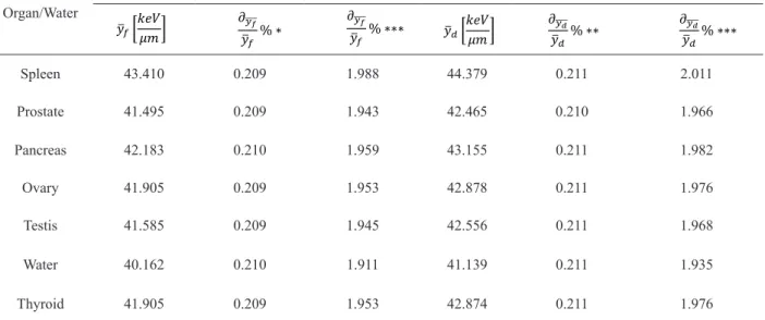
In order to compare different states, the frequency- mean lineal energy, dose-mean lineal energy, and these statistical uncertainties with the formulas 7, 14, and 16 and absorb dose in each case were calculated and reported, which its results are described in the next section.
1E-6 1E-5 1E-4 1E-3 0.01 0.1 1 10 100
0 20000 40000 60000 80000 100000
stopping power(MeV/m)
Energy(MeV)
water spleen Thyroid Pancreas
A
1E-6 1E-5 1E-4 1E-3 0.01 0.1 1 10 100
0 20000 40000 60000 80000 100000
stopping power(MeV/m)
Energy(MeV)
water Prostate Testis Ovary
B
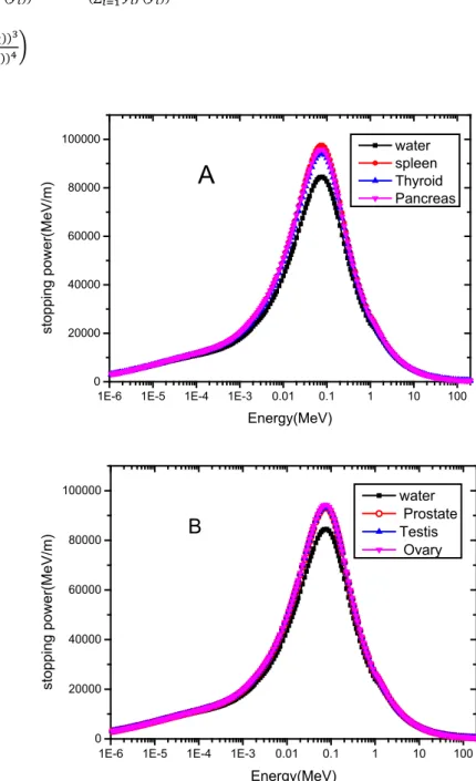
FIGURE 1. Stopping power curve versus proton energy in water (black curve) in comparison with organs of (a) spleen (red curve),
thyroid (blue curve) and pancreas (purple curve) (b) prostate (red curve), testis (blue curve), and ovary (purple curve)
( ) 1 𝜎𝜎𝑦𝑦̅̅̅̅2𝐷𝐷=∆𝑦𝑦1(∑𝑁𝑁𝑖𝑖=1𝑀𝑀𝑦𝑦𝑖𝑖4𝑓𝑓(𝑦𝑦𝑖𝑖)
12 −2 𝑆𝑆1∑𝑁𝑁𝑖𝑖=1𝑀𝑀𝑦𝑦𝑖𝑖3𝑓𝑓(𝑦𝑦𝑖𝑖)
13 +𝑀𝑀𝑆𝑆13
14) 𝜎𝜎𝑦𝑦̅̅̅̅2𝐷𝐷=∆𝑦𝑦1((∑∑𝑁𝑁𝑖𝑖=1𝑦𝑦𝑦𝑦𝑖𝑖4𝑓𝑓(𝑦𝑦𝑖𝑖)
𝑖𝑖𝑓𝑓(𝑦𝑦𝑖𝑖)
𝑁𝑁𝑖𝑖=1 )2−2 ∑ 𝑦𝑦(∑𝑖𝑖2𝑓𝑓(𝑦𝑦𝑖𝑖𝑦𝑦) ∑𝑁𝑁𝑖𝑖=1𝑦𝑦𝑖𝑖3𝑓𝑓(𝑦𝑦𝑖𝑖)
𝑖𝑖𝑓𝑓(𝑦𝑦𝑖𝑖)
𝑁𝑁𝑖𝑖=1 )3 +(∑(∑𝑁𝑁𝑖𝑖=1𝑦𝑦𝑦𝑦𝑖𝑖2𝑓𝑓(𝑦𝑦𝑖𝑖))3
𝑖𝑖𝑓𝑓(𝑦𝑦𝑖𝑖)
𝑁𝑁𝑖𝑖=1 )4)
( ) 1 𝜎𝜎𝑦𝑦̅̅̅̅2𝐷𝐷=∆𝑦𝑦1 (∑𝑁𝑁𝑖𝑖=1𝑀𝑀𝑦𝑦𝑖𝑖4𝑓𝑓(𝑦𝑦𝑖𝑖)
12 −2 𝑆𝑆1∑𝑁𝑁𝑖𝑖=1𝑀𝑀𝑦𝑦𝑖𝑖3𝑓𝑓(𝑦𝑦𝑖𝑖)
13 +𝑀𝑀𝑆𝑆13
14) 𝜎𝜎𝑦𝑦̅̅̅̅2𝐷𝐷=∆𝑦𝑦1 ((∑∑𝑁𝑁𝑖𝑖=1𝑦𝑦𝑦𝑦𝑖𝑖4𝑓𝑓(𝑦𝑦𝑖𝑖)
𝑖𝑖𝑓𝑓(𝑦𝑦𝑖𝑖)
𝑁𝑁𝑖𝑖=1 )2−2 ∑ 𝑦𝑦(∑𝑖𝑖2𝑓𝑓(𝑦𝑦𝑖𝑖𝑦𝑦) ∑𝑁𝑁𝑖𝑖=1𝑦𝑦𝑖𝑖3𝑓𝑓(𝑦𝑦𝑖𝑖)
𝑖𝑖𝑓𝑓(𝑦𝑦𝑖𝑖)
𝑁𝑁𝑖𝑖=1 )3 +(∑(∑𝑁𝑁𝑖𝑖=1𝑦𝑦𝑦𝑦𝑖𝑖2𝑓𝑓(𝑦𝑦𝑖𝑖))3
𝑖𝑖𝑓𝑓(𝑦𝑦𝑖𝑖)
𝑁𝑁𝑖𝑖=1 )4) (
) 1 𝜎𝜎𝑦𝑦̅̅̅̅2𝐷𝐷=∆𝑦𝑦1 (∑𝑁𝑁𝑖𝑖=1𝑀𝑀𝑦𝑦𝑖𝑖4𝑓𝑓(𝑦𝑦𝑖𝑖)
12 −2 𝑆𝑆1∑𝑁𝑁𝑖𝑖=1𝑀𝑀𝑦𝑦𝑖𝑖3𝑓𝑓(𝑦𝑦𝑖𝑖)
13 +𝑀𝑀𝑆𝑆13
14) 𝜎𝜎𝑦𝑦̅̅̅̅2𝐷𝐷=∆𝑦𝑦1 ((∑∑𝑁𝑁𝑖𝑖=1𝑦𝑦𝑦𝑦𝑖𝑖4𝑓𝑓(𝑦𝑦𝑖𝑖)
𝑖𝑖𝑓𝑓(𝑦𝑦𝑖𝑖)
𝑁𝑁𝑖𝑖=1 )2−2 ∑ 𝑦𝑦(∑𝑖𝑖2𝑓𝑓(𝑦𝑦𝑖𝑖𝑦𝑦) ∑𝑁𝑁𝑖𝑖=1𝑦𝑦𝑖𝑖3𝑓𝑓(𝑦𝑦𝑖𝑖)
𝑖𝑖𝑓𝑓(𝑦𝑦𝑖𝑖)
𝑁𝑁𝑖𝑖=1 )3 +(∑(∑𝑁𝑁𝑖𝑖=1𝑦𝑦𝑦𝑦𝑖𝑖2𝑓𝑓(𝑦𝑦𝑖𝑖))3
𝑖𝑖𝑓𝑓(𝑦𝑦𝑖𝑖)
𝑁𝑁𝑖𝑖=1 )4)