A Spatiotemporal Prediction Framework for Air Pollution Based on Deep RNN
Junxiang Fan a, b, *, Qi Li a, b, *, Junxiong Hou a, b, Xiao Feng a, Hamed Karimian a, Shaofu Lin ba Institute of Remote Sensing and GIS, Peking University, 100871 Beijing, China - [email protected] (J. Fan)
b Beijing Advanced Innovation Center for Future Internet Technology, Beijing University of Technology - [email protected] (Q. Li)
KEY WORDS: air pollution, missing value, RNN, LSTM, deep learning
ABSTRACT:
Time series data in practical applications always contain missing values due to sensor malfunction, network failure, outliers etc. In order to handle missing values in time series, as well as the lack of considering temporal properties in machine learning models, we propose a spatiotemporal prediction framework based on missing value processing algorithms and deep recurrent neural network (DRNN). By using missing tag and missing interval to represent time series patterns, we implement three different missing value fixing algorithms, which are further incorporated into deep neural network that consists of LSTM (Long Short-term Memory) layers and fully connected layers. Real-world air quality and meteorological datasets (Jingjinji area, China) are used for model training and testing. Deep feed forward neural networks (DFNN) and gradient boosting decision trees (GBDT) are trained as baseline models against the proposed DRNN. Performances of three missing value fixing algorithms, as well as different machine learning models are evaluated and analysed. Experiments show that the proposed DRNN framework outperforms both DFNN and GBDT, therefore validating the capacity of the proposed framework. Our results also provides useful insights for better understanding of different strategies that handle missing values.
* Corresponding author
1. INTRODUCTION
Air pollution remains a serious concern in developing countries such as China and India and has attracted much attention. Typical sources of air pollution include industrial emission and traffic emission, and the main pollutants are PM2.5, PM10, NO2,
SO2, O3 etc. Among the pollutants PM2.5 has attracted immense
attention. PM2.5 is fine particulate matter or particles that are
less than 2.5 micrometers in diameter, usually consisting of solid or liquid particles. The correlation between health risk and the concentration of air pollutants have been studied (Stieb et al., 2008, Chen et al., 2013). Organizations and governments, such as the World Health Organization (WHO, 2006), the USA Environmental Protection Agency (Laden et al., 2000), Japan (Wakamatsu et al., 2013) have implemented policies to support air pollution countermeasures.
Presently the models for predicting air pollutants can be classified into two types. The first type includes mechanism models that tracks the generation, dispersion and transmission process of pollutants, and predictive results are given by numerical simulations. Two commonly used mechanism models are CMAQ (Byun & Ching, 1999) and WRF/Chem (Grell et al., 2005). Both of these two models incorporate physical and chemical models. Physical models are used to generate meteorological environment parameters, while chemical models are for pollutant transmission simulations. The second type of models usually used in air pollution predictions are statistical learning models or machine learning models. These models attempt to find patterns directly from the input data, rather than numerical simulations. Some of the widely used models are linear regression, Geographically Weighted Regression (Ma et al., 2014), Land Use Regression (Eeftens et al., 2012), Support Vector Machine (Osowski et al., 2007) and Artificial Neural Networks (Voukantsis et al., 2011, Feng et al., 2015). Various attempts have also been made to combine different methods in order to achieve better performance (Sanchez et al., 2013; Adams & Kanaroglou, 2016). A form of neural networks known
as recurrent neural networks (RNN) has exhibited very ideal performance in modelling temporal structures (Graves & Schmidhuber, 2009, Lipton et al., 2015). While open datasets grow more rapidly than ever, traditional machine learning methods may not be able to depict complex patterns within the massive datasets. But since the difficulty of training huge neural networks has been alleviated (Hinton & Salakhutdinov, 2006, Hinton et al., 2006), and hardware developments grants researchers stronger computational resources, constructing deep neural networks (DNN) for learning complex patterns has become possible.
On the other hand, forecasting air pollution requires time series data, which may contain discontinuities due to malfunction of sensors, delay of networks etc. Therefore the gaps within data must be handled before training machine learning models. Various solutions have been proposed to alleviate the missing data problem, including smoothing, interpolation and kernel methods (Kreindler et al., 2006; White et al., 2011, Rehfeld et al., 2011). But many of these methods require knowledge of the full dataset before fixing gaps, so the fixing phase and model training phase have to be separated. This may influence the efficiency in a real world application.
In this paper, our goal is to develop a spatiotemporal framework that is able to deal with missing values in time series data. To exploit the informative missingness patterns, we design three real-time/semi real-time interpolation algorithms. Then we introduce a spatiotemporal prediction framework incorporating deep recurrent neural networks (DRNN) and the interpolation algorithms. Numerical results demonstrate that our proposed DRNN outperforms strong baseline models including deep feed forward neural networks and GBDT. The main contributions of this paper as follows:
(a) We introduce three missing value fixing algorithms by characterizing the missing patterns of not missing-completely-at-random time series data.
(b) We propose a general spatiotemporal framework based on deep recurrent neural works (DRNN), that takes advantage of both spatial and temporal correlations. The capacity of the framework is further enhanced by the fixing algorithms.
2. PROBLEM STATEMENT AND KEY MODELS 2.1 Spatiotemporal Forecasting
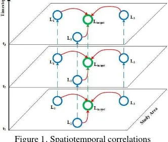
Both spatial and temporal information should be considered when forecasting the spatiotemporal distribution of air pollutants. Firstly, the air quality data at given spatial point or within certain area has internal temporal correlation. Historical states can affect current and future states, e.g. the air quality during the last hour will affect the air quality during the next hour. Secondly, air pollutants may disperse or transmit through the atmosphere, and this process is highly related to wind direction and wind speed, therefore air quality of adjacent areas will also influence the local air quality. In order to construct a precise forecasting model, both spatial and temporal correlations should be taken into account. The sources of air pollutants can be classified into two different types: local source of emission and outside emission that transported into local area, and their properties can be depicted by temporal and spatial correlations, respectively. Spatial and temporal correlations are illustrated in figure 1, where blue circles represent adjacent points, green circles represent target point, dashed lines are the temporal correlations between local air quality conditions, and the red arrows are spatial correlations.
Figure 1. Spatiotemporal correlations
For N different monitoring stations, the input dataset can be
denoted as N time series, ST={
st
1,st
2 ,…,st
N }, wheren
st
={X1,X2,…,XT}(n=1,…,N) is the data sequence of a singlestation n (T timesteps), and each observation Xt in the sequence
is a d dimensional vector. Therefore the spatiotemporal forecasting task can be defined as: At given timestep t, find a subset STsub of ST for target station n. Then predict the value of
n on timestep (t+1,t+2,…,t+F) based on the historical records of
n
st
∪STsub at timestep (t,t-1,…,t-H). We can use the neareststations from station n as the subset, so that the spatial correlations are reflected in the model. The input of the forecasting system is the historical data, including air quality data and meteorological data, and the output is the air pollutant prediction value for single stations. Spatial distribution for the whole research area can be generated by interpolating prediction values. The data flow of spatiotemporal forecasting is shown in figure 2 (nn1/nn2/nn3 denote the three nearest neighbouring stations of station n).
Figure 2. Data flow of spatiotemporal forecasting
2.2 Fixing Missing Values
One way of handling missing values in time series prediction is to directly omit the missing sections, and use only the consecutive parts. But this method is only applicable when missing values do not occur randomly and frequently. Also, the missing pattern of time series data may also contain information that could improve the performance of model prediction. The other option is to fix the missing values by resampling or interpolation, but these methods may require knowledge of the whole dataset before dealing with missing data, and may result in a two-staged modelling process (Wells et al., 2013). Recent works tried to model explicitly the missingness of various datasets (Wu et al., 2015), or interpolate according to the time series information of missing data in health care dataset (Che et al., 2016). We implemented three missing value fixing methods based on similar ideas for air pollution time series data. These methods are real-time or semi real-time because the missing data can be fixed in an “online” or batched fashion.
Let
st
n={X1,X2,…,XT} be a time sequence with missing values. dimension, which is the number of timesteps since the last time this dimension has valid value.
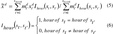
td can be represent as belowWe implemented and compared three different interpolation methods for fixing missing values in air quality data sequence: (a) Fix the missing values using the latest valid observation sees the whole dataset, therefore it is a real-time algorithm. (b) Fix the missing values using mean value of the same time point in the whole month (mean-fix).
d
dWhere
~
x
d denotes the average value of all valid obervations of the dth dimension at the same timepoint each day in the same month. The method produces substitution of missing values after reading data for a whole month, so it is semi real-time.
(c) Fix the missing values using a weighted sum of (a) and (b). The logic is that for a given observation variable, there could be a long term default value, but it could also be affected by sudden changes. Therefore by assigning a exponential decay weight, we can combine latest observation and long term average value. In this combination, the effect of latest valid observation decreases as the missing period extends. Since it combines the two methods above, it is a semi real-time method.
d neural network (FNN): FNN consists of layers stacked on top of each other, where each layer is composed of neurons, and all connections between layers follow the same direction. RNN introduces cyclic structure into the network, which is implemented by connection of neurons. By using self-connected neurons, historical inputs can be ‘memorized’ by RNN and therefore influence the network output. The ‘memory’ that RNN holds enables it to outperform FNN in many real-world applications.The inference process of RNN is similar to that of FNN, which is finished by forward propagation. Training of FNN is done by back propagation (BP) algorithm. While RNN models sequence data and takes the transfer of ‘memory’ into account, therefore its training process should stack BP results over time dimension, resulting in the back propagation through time (BPTT) algorithm.
For a basic RNN structure composed of one input layer of I neurons, one hidden layer of H neurons and one output layer of K neurons, its forward and back propagations are as below. The input of the network is a sequence X of length T.
The forward propagation process is as follows:
represents the activation function of neuron h. The BPTT algorithm of RNN is as follows:
t timesteps, gradient may tend to be 0, leaving the parameters of a network with long-term dependency hard to train (Bengio et al., 1994; Hochreiter et al., 2001). This problem is called ‘vanishing gradient’.
In order to solve the vanishing gradient problem, the Long Short-Term Memory (LSTM) structure was introduced (Hochreiter & Schmidhuber, 1997). LSTM has the similar basic structure as RNN, but the neurons are replaced by memory blocks. Each memory block contains one or more memory cells and three nonlinear units (gates): input gate, output gate and forget gate. By doing matrix multiplication, the input gate, output gate and forget gate controls the input, output and state reset of the memory cell, respectively. Two kinds of information flow exist within LSTM, the first is from each memory block to other blocks/neurons, e.g. the output value of memory cell. And the second is within the same memory block, e.g. the cell state or ‘memory’ of the memory cell, the input of the memory cell, and the activation of each gate unit. The gates ensure that gradient information of LSTM will not vanish through back propagation, thus enable LSTM to learn dependencies across long time period. Parameters of LSTM are trained using BPTT. Core structure of LSTM is illustrated as follows (Graves, 2012):
Figure 3. Structure of LSTM memory block
3. EXPERIMENTS 3.1 Data Description
The study area is Jingjinji area of northern China, which suffers from severe air pollution events that frequently occur during heating seasons. The data comes from APIs provided by the Ministry of Environmental Protection of PRC and China Meteorological Administration. Two kinds of original data are used: (a) air quality data, including air quality records from monitoring stations, and station information, (b) meteorological data at county level. There are 80 air quality monitoring stations and 25 corresponding counties for meteorological data in Jingjinji area. Our dataset covers the period from September 2013 to January 2015, and by performing fixing algorithms, we make up of the discontinuous parts of the original data. Statistics of the data before and after fixing are shown in table 1. ISPRS Annals of the Photogrammetry, Remote Sensing and Spatial Information Sciences, Volume IV-4/W2, 2017
Type Before Fixing After Fixing Missing Rate
Air Quality 826930 911660 10%
Meteorology 446228 460141 4%
Table 1. Statistics of data before and after fixing missing values.
3.2 Methods and Implementation Details
In our proposed framework, spatial and temporal correlations are represented by neighbouring stations and the ‘memory’ of LSTM, respectively. The final input includes 5 kinds of information: (a) local air quality properties, e.g. PM2.5, PM10,
O3, SO2, NO2, CO, (b) local meteorological properties, e.g.
temperature, wind direction, wind speed, humidity, (c) air quality of neighbouring stations, (d) time properties, e.g. weekday, date, month and hour, (e) spatial properties, e.g. longitude and latitude of stations. The dimensions of inputs are as follows:
Variable unit
PM2.5 μg/m3
PM10 μg/m3
O3 ppb
SO2 ppb
NO2 ppb
CO ppb
Temperature °C
Wind_direction NA
Wind_speed NA
humidity NA
weekday NA
month NA
day NA
hour NA
longitude °
latitude °
Nearest Neighbour1 PM2.5 μg/m3
Nearest Neighbour 2 PM2.5 μg/m3
Nearest Neighbour 3 PM2.5 μg/m3
Table 2. Features of input data
Our model predicts the future 1~8 hour PM2.5 concentration
based on the historical records from the past 48 hours. Therefore the raw data should be re-organized to generate a time dimension after fixing missing values. Data from January 2014 to January 2015 is used, 60% of is used as training set, 20% used as validation set and 20% used as test set.
The models that are implemented and evaluated can be categorized into three following groups:
(a) Non-RNN Machine Learning Baselines: We evaluate GBDT (Gradient Boosting Decision Tree) which is widely used in both regression and classification problem, and outperforms many other models in generalization ability.
(b) Non-RNN Deep Learning Baselines: We take deep feed forward neural networks which share the number of layers with the deep recurrent neural networks that we propose as baselines. (c) Proposed Deep Learning Methods: This is our proposed model based on LSTM.
On top of three kinds of missing value fixing algorithms (forward-fix/mean-fix/decay-fix), we propose two deep neural networks based on LSTM (DRNN-1 & DRNN-2). GBDT and two deep feed forward neural networks (DFNN-1 & DFNN-2) are used as baseline models. DFNN shares the basic structure with DRNN, but all layers of DFNN are fully-connected layers. Network structure of DFNN1, DFNN2, DRNN1 and DRNN2 are shown in figure 4. Structure details of GBDT and neural networks are provided in table 3 and table 4, respectively.
a DFNN1 b DFNN2
(c) DRNN1 (d) DRNN2
Figure 4. Structrures of proposed deep neural networks and baseline models. (a) DFNN1, (b) DFNN2, (c) DRNN1, (d)
DRNN2.
parameter Value
Number of trees 100
Depth of tree 4
Shrinkage 0.1
Loss function Mean Square Error
Table 3. Parameters of GBDT
Fix method Network Name Layers
Forward DRNN1forward 1 LSTM + 2 Dense DRNN2forward 2 LSTM + 2 Dense
DFNN1forward 3 Dense
DFNN2forward 4 Dense
Mean DRNN1mean 1 LSTM + 2 Dense
DRNN2mean 2 LSTM + 2 Dense
DFNN1mean 3 Dense
DFNN2mean 4 Dense
decay DRNN1decay 1 LSTM + 2 Dense DRNN2decay 2 LSTM + 2 Dense
DFNN1decay 3 Dense
DFNN2decay 4 Dense
Table 4. Structures of deep neural networks Training details of the deep neural networks are as follows:
Parameter Value
Number of Records 597727
Time Interval 1
Training set 60%
Validation set 20%
Test set 20%
Prediction Length (F, hour) 1~8
History Length (L, hour) 48
Number of nearest neighbours 3
Parameter Update RMSprop
Training Epochs 100
Batch Size DRNN/DFNN:256/32
Loss Function Mean Square Error
Table 5. Training details of deep neural networks
Deep neural networks may suffer the problem of overfitting, therefore we use dropout to regularize the neural networks, and the basic idea is to randomly remove neurons and connections from network during training (Srivastava et al., 2014). In our model, the dropout rate is set to 0.1.
Performances of each model is measured by RMSE, MSE and IA (index of agreement) defined below:
n
i i
i y
y n RMSE
1
2
ˆ
1 (14)
n
i i i y
y n MAE
1
ˆ
1 (15)
Index of agreement is an dimensionless index proposed by Willmott to assess the average loss of model predictions (Willmott, 1981):
n
i
i i
n
i i i
O O O P
O P IA
1
2 1
2
1
(16)
The proposed models and baseline models are implemented using Python, Theano, Keras and Scikit-learn (Al-Rfou et al., 2016; Chollet, 2015; Pedregosa, 2011), and executed on a computer with Intel Core i5-4590 CPU 3.30 GHz, 16 GB RAM and NVIDIA GeForce GTX 750 Ti graphics card.
3.3 Quantitative Results and Discussion
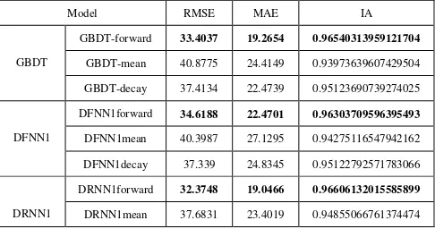
Precision measurements of models when performing 1 and 8 hours prediction are provided separately in table 6 and table 7 (measurements for 2~7 hours prediction are not presented due to length limit of this paper).
Model RMSE MAE IA
GBDT
GBDT-forward 33.4037 19.2654 0.96540313959121704 GBDT-mean 40.8775 24.4149 0.93973639607429504 GBDT-decay 37.4134 22.4739 0.95123690739274025
DFNN1
DFNN1forward 34.6188 22.4701 0.96303709596395493 DFNN1mean 40.3987 27.1295 0.94275116547942162 DFNN1decay 37.339 24.8345 0.95122792571783066
DRNN1
DRNN1forward 32.3748 19.0466 0.96606132015585899 DRNN1mean 37.6831 23.4019 0.94855066761374474
DRNN1decay 34.7096 21.5057 0.9573289193212986
DFNN2
DFNN2forward 32.078 19.0256 0.96985132247209549 DFNN2mean 38.6887 24.1764 0.9470319040119648 DFNN2decay 35.4674 22.1008 0.95896736159920692
DRNN2
DRNN2forward 29.0978 16.5493 0.97368617355823517 DRNN2mean 31.172 18.8931 0.96755732223391533 DRNN2decay 29.476 17.5485 0.9715470764786005
Table 6. Model accuracy of proposed models and baseline models for 1-hour prediction.
Model RMSE MAE IA
GBDT
GBDT-forward 60.1087 40.018 0.85550019145011902 GBDT-mean 60.2848 40.7778 0.83446812629699707 GBDT-decay 59.0271 39.6728 0.8464382141828537
DFNN1
DFNN1forward 51.5646 35.5507 0.91059249639511108 DFNN1mean 53.0535 36.7613 0.8925386369228363 DFNN1decay 52.3769 36.2841 0.89876601099967957
DRNN1
DRNN1forward 49.1941 33.5947 0.9178883358836174 DRNN1mean 50.6616 35.2142 0.90207912027835846 DRNN1decay 48.6082 33.6893 0.91163397580385208
DFNN2
DFNN2forward 44.9636 30.3586 0.93633241951465607 DFNN2mean 47.87 32.5431 0.91608843207359314 DFNN2decay 45.3751 30.8343 0.92688383907079697
DRNN2
DRNN2forward 35.7362 23.721 0.96116474643349648 DRNN2mean 38.1375 25.3731 0.95056585595011711 DRNN2decay 36.6295 24.3019 0.95535894483327866
Table 7. Model accuracy of proposed models and baseline models for 8-hour prediction.
From the comparisons we may obtain two basic conclusions: (a) In short-time prediction (< 4 hours), the models that are based on forward-fix have the best performance, and models based on mean-fix are poorer than those based on forward-fix or decay-fix. (b) With the same input data and similar network structure, deep recurrent neural networks get better results than deep feed forward neural networks and GBDT.
A possible explanation for the first conclusion is that air pollution events in Jingjinji area are mostly due to sudden changes of atmosphere conditions. Therefore when doing short-time predictions, forward-fix can always stay close to the original air quality fluctuation trend, while mean-fix may over-smooth the sudden events in original data, resulting in a less precise model. But for the performances of long-time predictions (≥ 4 hours), models based on forward-fix may not always be the best choice. For some long-time prediction tasks, both DRNN1 and DRNN2 achieve best results when using decay-fix. This is illustrated in figure 5 and figure 6.
Figure 5. RMSE of DRNN1 models
Figure 6. RMSE of DRNN2 models
When using DRNN1 to predict PM2.5 concentrations for 7~8
hours in the future, it achieves best result when using decay-fix. While DRNN1 has the best performance with decay-fix when predicting for 4~5 hours in the future. These figures illustrate that considering the long-term average pattern may also improve the performance of predicting models.
As for the second conclusion, we can get some more profound results if we compare different models based on the same fixing algorithm. Below are the performance measurements of models based on decay-fix method:
Prediction Length
GBDT-decay
DFNN1 decay
DFNN2 decay
DRNN1 decay
DRNN2 decay 1h 37.4134 37.339 35.4674 34.7096 29.476 2h 43.7124 41.8736 40.0298 39.7054 34.1725 3h 47.361 44.6763 41.9434 42.8865 38.1135 4h 51.0985 47.6545 44.1036 46.5324 37.0615 5h 53.8403 48.9523 44.9586 46.8369 35.9535 6h 55.9714 49.9253 45.2652 47.4329 36.7823 7h 58.0017 50.9427 45.7488 48.2162 37.3184 8h 59.0271 52.3769 45.3751 48.6082 36.6295
Table 8. Accuracy of models based on decay-fix
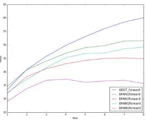
Performances of models based on three fix methods are illustrated in figure 7~9 below.
Figure 7. RMSE of models based on forward-fix
Figure 8. RMSE of models based on mean-fix
Figure 9. RMSE of models based on decay-fix
Based on table 8 and figure 7~9, we find that prediction models based on deep neural networks (DFNN/DRNN) have better performances than traditional machine learning methods (GBDT). While basic structures are similar, DRNN has better predicting power than DFNN, e.g. both DRNN1 and DRNN2 achieve higher precisions than DFNN2 when predicting for 2 hours in the future.
DRNN has better explanation capacity than the others. Possible explanation could be that the model abstracts input data as sequential states, and transmits the states through timesteps, while DFNN and GBDT cannot explicitly model the temporal states. The difference also results in higher loss of precision for DFNN and GBDT when predicting length extends.
Training and validation loss of methods based on forward-fix are illustrated in figure below. The training process of DFNN is less stable than DRNN. Although increasing layers may improve model performances, the improvement for DFNN is lower than DRNN.
(a) DFNN1forward (b) DFNN2forward
(c) DRNN1forward (d) DRNN2forward
Figure 10. Training and validation loss of models based on forward-fix. (a) DFNN1forward, (b) DFNN2forward, (c)
DRNN1forward, (d) DRNN2forward
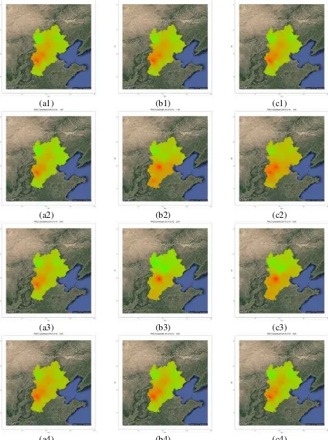
By spatially interpolating the time series prediction results, we can get the spatiotemporal distribution of air pollutants in the study area. One heavy pollution event was reported on November 10th, 2014, therefore we use the proposed DRNN2
based on three fixing algorithms to generate hourly predictions of PM2.5, and compare their forecasting performances. The
PM2.5 concentration at each station 1 hour in the future is
predicted, using historical data from the past 48 hours, then we use inverse distance weighted interpolation to generate spatial distribution at each future time point.
The predicted spatiotemporal PM2.5 distributions from 0:00 to
3:00 a.m. on that day are illustrated in figure 11.
(a1) (b1) (c1)
(a2) (b2) (c2)
(a3) (b3) (c3)
(a4) (b4) (c4)
Figure 11. Prediction distribution of PM2.5 by DRNN2 models
from 0:00 to 3:00 a.m. on 12/10/2014. (a) forward-fix, (b) mean-fix, (c) decay-fix.
According to history data, records between 1:00 am to 2:00 am were missing on November 10th, 2014, and the heavy pollution
events starts on November 9th. Our results show that the region
around Shijiazhuang (station id 1028A) should be heavily polluted during the missing period, but prediction results of mean-fix based method only shows light pollution, while the other two methods predicts the heavy pollution successfully. This is consistent with our assumption that methods based on mean-fix tend to smooth out the trend between 1:00 am to 2:00 am.
By plotting the spatial distribution of meteorological conditions, we can also find some other properties of air pollutions in this area: (a) Spatiotemporal distribution of humidity has real-time correlation with PM2.5, which is consistent with the
requirements of smog generation. (b) Negative correlation exists between wind speed and PM2.5 concentration, and the
correlation has a 1~2 hours’ lag, suggesting that smog in the area is highly affected by wind.
4. CONCLUSIONS
In this paper, we proposed novel deep learning frameworks that can efficiently handle missing values in spatiotemporal forecasting tasks. The motivation is that real-world time series dataset is prone to be discontinuous, and models can be enhanced if the gaps within data are fixed properly. In light of this, we proposed three real-time/semi real-time fixing methods that impute the missing values in an ‘online’ or ‘batch’ way. We have then introduced a deep recurrent neural network constructed with LSTM on top of the fixing methods. Numerical results on datasets of Jingjinji area showed that by taking advantage of the ‘memory’ property, neural networks with LSTM outperforms baseline models such as deep feed forward neural networks and GBDT. Our DRNN framework can predict both sudden heavy pollution events and average patterns with relatively high precisions. Performances of three fixing methods revealed that forward-fix is generally the best choice among the three methods, which is consistent with the fact that air pollution in Jingjinji area are often caused by sudden changes of atmosphere environments. But decay-fix may achieve better results than the other two in long time predictions (4~8 hours), showing that adding long term average patterns may improve model accuracy.
ACKNOWLEDGEMENTS (OPTIONAL)
This work was supported by the National Key Technology R&D Program of the Ministry of Science and Technology of China (Grant No. 2012BAC20B06).
REFERENCES
Adams, Matthew D., and Pavlos S. Kanaroglou. "Mapping real-time air pollution health risk for environmental management: Combining mobile and stationary air pollution monitoring with neural network models." Journal of environmental management 168 (2016): 133-141.
Al-Rfou, Rami, et al. "Theano: A Python framework for fast computation of mathematical expressions." arXiv preprint arXiv:1605.02688 (2016).
Bengio, Yoshua, Patrice Simard, and Paolo Frasconi. "Learning long-term dependencies with gradient descent is difficult." IEEE transactions on neural networks 5.2 (1994): 157-166.
Byun, Daewon W., and J. K. S. Ching, eds. Science algorithms of the EPA Models-3 community multiscale air quality (CMAQ) modeling system. Washington, DC: US Environmental Protection Agency, Office of Research and Development, 1999.
Chen, Renjie, et al. "Communicating air pollution-related health risks to the public: an application of the Air Quality Health Index in Shanghai, China." Environment international 51 (2013): 168-173.
Che, Zhengping, et al. "Recurrent neural networks for multivariate time series with missing values." arXiv preprint arXiv:1606.01865 (2016).
Eeftens, Marloes, et al. "Development of land use regression models for PM2. 5, PM2. 5 absorbance, PM10 and PMcoarse in 20 European study areas; results of the ESCAPE project." Environmental science & technology 46.20 (2012): 11195-11205.
Feng, Xiao, et al. "Artificial neural networks forecasting of PM 2.5 pollution using air mass trajectory based geographic model and wavelet transformation." Atmospheric Environment 107 (2015): 118-128.
François Chollet. Keras. GitHub repository: https://github.com/fchollet/keras, 2015.
Graves, Alex. "Supervised sequence labelling." Supervised Sequence Labelling with Recurrent Neural Networks. Springer Berlin Heidelberg, 2012. 5-13.
Graves, Alex, and Jürgen Schmidhuber. "Offline handwriting recognition with multidimensional recurrent neural networks." Advances in neural information processing systems. 2009.
Grell, Georg A., et al. "Fully coupled “online” chemistry within the WRF model." Atmospheric Environment 39.37 (2005): 6957-6975.
Hinton, Geoffrey E., and Ruslan R. Salakhutdinov. "Reducing the dimensionality of data with neural networks." science 313.5786 (2006): 504-507.
Hinton, Geoffrey E., Simon Osindero, and Yee-Whye Teh. "A fast learning algorithm for deep belief nets." Neural computation 18.7 (2006): 1527-1554.
Hochreiter, Sepp, and Jürgen Schmidhuber. "Long short-term memory." Neural computation 9.8 (1997): 1735-1780.
Hochreiter, Sepp, et al. "Gradient flow in recurrent nets: the difficulty of learning long-term dependencies." (2001).
Kreindler, David M., and Charles J. Lumsden. "The effects of the irregular sample and missing data in time series analysis." Nonlinear Dynamical Systems Analysis for the Behavioral Sciences Using Real Data (2012): 135.
Laden, Francine, et al. "Association of fine particulate matter from different sources with daily mortality in six US cities." Environmental health perspectives 108.10 (2000): 941.
Lipton, Zachary C., John Berkowitz, and Charles Elkan. "A critical review of recurrent neural networks for sequence learning." arXiv preprint arXiv:1506.00019 (2015).
Ma, Zongwei, et al. "Estimating ground-level PM2. 5 in China using satellite remote sensing." Environmental science & technology 48.13 (2014): 7436-7444.
Osowski, Stanislaw, and Konrad Garanty. "Forecasting of the daily meteorological pollution using wavelets and support vector machine." Engineering Applications of Artificial Intelligence 20.6 (2007): 745-755.
Pedregosa, Fabian, et al. "Scikit-learn: Machine learning in Python." Journal of Machine Learning Research 12.Oct (2011): 2825-2830.
Rehfeld, Kira, et al. "Comparison of correlation analysis techniques for irregularly sampled time series." Nonlinear Processes in Geophysics 18.3 (2011): 389-404.
Sánchez, Antonio Bernardo, et al. "Forecasting SO2 pollution incidents by means of Elman artificial neural networks and ARIMA models." Abstract and Applied Analysis. Vol. 2013. Hindawi Publishing Corporation, 2013.
Srivastava, Nitish, et al. "Dropout: a simple way to prevent neural networks from overfitting." Journal of Machine Learning Research 15.1 (2014): 1929-1958.
Stieb, David M., et al. "A new multipollutant, no-threshold air quality health index based on short-term associations observed in daily time-series analyses." Journal of the Air & Waste Management Association 58.3 (2008): 435-450.
Voukantsis, Dimitris, et al. "Intercomparison of air quality data using principal component analysis, and forecasting of PM 10 and PM 2.5 concentrations using artificial neural networks, in Thessaloniki and Helsinki." Science of the Total Environment 409.7 (2011): 1266-1276.
Wakamatsu, Shinji, Tazuko Morikawa, and Akiyoshi Ito. "Air pollution trends in Japan between 1970 and 2012 and impact of urban air pollution countermeasures." Asian Journal of Atmospheric Environment 7.4 (2013): 177-190.
Wells, Brian J., et al. "Strategies for handling missing data in electronic health record derived data." eGEMs 1.3 (2013).
White, Ian R., Patrick Royston, and Angela M. Wood. "Multiple imputation using chained equations: issues and guidance for practice." Statistics in medicine 30.4 (2011): 377-399.
Willmott, Cort J. "On the validation of models." Physical geography 2.2 (1981): 184-194.
World Health Organization. Air quality guidelines: global update 2005: particulate matter, ozone, nitrogen dioxide, and sulfur dioxide. World Health Organization, 2006.
Wu, Shin-Fu, Chia-Yung Chang, and Shie-Jue Lee. "Time series forecasting with missing values." Industrial Networks and Intelligent Systems (INISCom), 2015 1st International Conference on. IEEE, 2015.