www.elsevier.com/locate/dsw
An optimal replenishment policy for deteriorating items with
time-varying demand and partial–exponential
type – backlogging
S. Papachristos
a;∗, K. Skouri
baDepartment of Mathematics, Statistics and Operational Research Section, University of Ioannina, 45110 Ioannina, Greece bDepartment of Mathematics, University of Ioannina, 45110 Ioannina, Greece
Received 1 July 1999; received in revised form 1 June 2000; accepted 1 June 2000
Abstract
We study a continuous review inventory model over a nite-planning horizon with deterministic varying demand and constant deterioration rate. The model allows for shortages, which are partially backlogged at a rate which varies exponentially with time. For this model an optimal replenishment policy is established. c 2000 Elsevier Science B.V. All rights reserved.
Keywords:Inventory; Lot sizing; Deterioration; Shortage; Partial backlogging
1. Introduction
The deterioration of many items during storage period is a real fact. Foods, pharmaceuticals, chemicals, blood, drugs are a few examples of such items. Chare and Schrader [9], rst, proposed an inventory model having a constant rate of deterioration and a constant rate of demand over a nite-planning horizon. Covert and Phillip [4] extended Chare and Schrader’s model by considering variable rate of deterioration. Shah [15] suggested a further generalization of all these models by allowing shortages and using a general distribution for the deterioration rate. The common characteristic of these articles was that demand rate was taken as a constant over the whole planning horizon.
The assumption of a constant demand rate is usually valid in the mature stage of the life cycle of the product. In the growth and=or end stage of the product life cycle demand rate can be well approximated by a linear function. Donaldson [7] developed an exact replenishment policy concerning this case.
Dave and Patel [6] studied an inventory model with deterministic but linearly changing demand rate and constant deterioration rate over a nite planning horizon. In their formulation they assumed replenishment
∗Corresponding author. Fax: +30-651-98297. E-mail address: spapachr@cc.uoi.gr (S. Papachristos).
results by introducing a logconcave function to describe the demand rate. Chakrabarti and Chaudhurri [3] studied an inventory model with linearly changing demand rate, constant deterioration rate and shortages over a nite-planning horizon. In their model they assumed cycles of equal lengths (each cycle starts with shortages) and the initial and nal inventory levels are both zero. Teng et al. [16] presented an inventory model under a general-demand function constant deterioration rate and shortages over a nite-planning horizon. Moreover, their model starts with shortages and ends with shortages. The characteristic of all the above articles is that they allow shortages, while unsatised demand is completely backlogged.
For models where shortages are allowed, complete backlogging, or complete loss of unsatised demand are two extreme cases. So researchers have turned their attention to models that allow partial backlogging, (e.g. Wee [17,18]).
In this article, we develop an EOQ inventory model over a nite planning horizon, with constant deteri-oration rate, time-varying demand rate and time-dependent partial backlogging. More explicitly, we suppose that the rate of backlogged demand increases exponentially as the waiting time for the next replenishment decreases. We believe that this is a quite reasonable assumption since as the waiting time decreases, more and more customers are willing to wait to get their orders as soon as the backlogged demand reaches the system at the next replenishment.
The paper is organized as follows. In Section 2 we give the assumptions of the model and the notation used. We continue with the mathematical formulation of the model in Section 3. In Section 4 we present results, theorems and lemmas, which ensure the existence of the optimal plan and we give the algorithm that can be used to nd the parameters of the optimal policy. The paper continues with Section 5 where we give a numerical example, explaining the procedure proposed in Section 4. Some comments and conclusions are given in Section 6. The paper closes with an appendix where we provide proofs for some of the results stated in previous sections.
2. Assumptions and notation
The inventory model is a continuous review model developed under the following assumptions:
1. The planning horizon of the system is nite and is taken asH time units. The initial and the nal inventory
levels are both zero during this time horizon.
2. Replenishment is instantaneous (replenishment rate is innite). 3. The lead time is zero.
4. The on hand inventory deteriorates at a constant rate (0¡ ¡1) per time unit. The deteriorated items
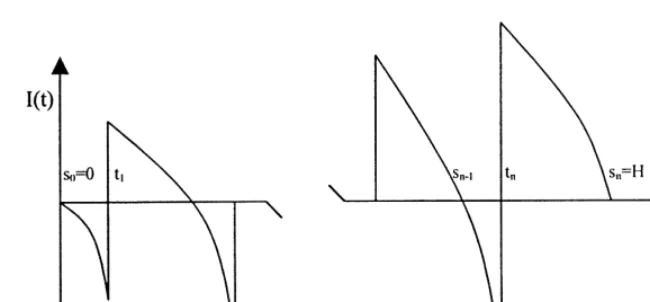
Fig. 1. Graphical representation of inventory.
5. The rate of demand,f(t); t∈[0; H]; is a continuous, logconcave function of t; withf′
(t)6= 0∀t.
6. The system allows for shortages in all cycles and each cycle starts with shortages.
7. Unsatised demand is backlogged at a rate exp(−x); wherexis the time up to the next replenishment and
a parameter 0¡ ¡(1=H).
Nomenclature
C the replenishment cost per order.
C1 holding cost per unit of stock carried per unit time.
C2 shortage cost per unit of shortage per unit time.
C3 deterioration cost per unit of deteriorated items.
CIi the amount of inventory carried during the ith cycle.
DIi the amount of deteriorated items during the ith cycle.
SIi the amount of units in shortages during the ith cycle.
I(t) the inventory level at time t.
n the number of replenishment cycles during the planning horizon.
si time at which shortage starts during the ith cycle i= 1; : : : ; n−1.
ti time at which the ith replenishment is madei= 1; : : : ; n.
Ti length of the ith cycle
3. Mathematical formulation of the model
The uctuation of the inventory level in the system is given in Fig. 1. The depletion of inventory during
the interval [ti; si]; of theith replenishment cycle, is due to the joint eect of the demand and the deterioration
of items. Hence the dierential equation, which describes the variation of inventory level, I(t); with respect
to time t; is
dI(t)
dt =−I(t) −f(t); ti6t ¡ si (1)
with boundary condition I(si) = 0; i= 1; : : : ; n.
The solution of (1) is
I(t) = e−tZ si t
with boundary condition I(si−1) = 0; i= 1; : : : ; n.
The solution of (5) is
I(t) =−
Z t
si−1
e−(ti−u)f(u) du; s
i−16t ¡ ti: (6)
From (6) the amount of shortage during the ith cycle is given by
SIi=
Now, we have all quantities needed to formulate the total inventory cost as the sum of ordering, holding,
deterioration and shortage cost, for any policy with n replenishments:
TC(n; si; ti) =nC+C1
The goals of this paper are: (1) to present an algorithm which, for a given number of replenishments, n;
can be used to determine the optimal replenishment points, t∗
i, and the optimal shortage points, s
∗
i and (2) to
obtain the overall optimal policy, i.e. nd the optimal values for the parameters, n; ti and si.
4. The optimal replenishment procedure
In this section, we shall present all the results which will lead to the construction of the algorithm giving the
optimal ti; si; values, for any policy withn replenishments. The continuity off(t) guarantees that TC(n; si; ti)
is a continuous function of si; ti and its rst- and second-order partial derivatives exist.
In Appendix A we prove that the solution, t∗
i; s
∗
i; i= 1;2; : : : ; n; of the above system of equations, satises
the second-order conditions for a minimum. Moreover, as we shall see, the system of equations (9), (10) has a unique solution and so the above minimum is a global minimum.
We shall now present the methodology used to solve Eqs. (9) and (10), and after that, we shall prove
that the obtained solution is unique. It is easy to see that, once t1 is known s1(t1) can be obtained from (9).
Then t2(t1) can be obtained from (10) and following this alternate procedure we can nd s2(t1); : : : ; sn(t1).
Similarly, if we start with tn; as known, sn−1(tn) can be obtained from (9), tn−1(tn) can be obtained from
(10) and repeating this procedure we can determine sn−2(tn); tn−2(tn); : : : ; t1(tn) and s0(tn). It is obvious that
the optimal replenishment policy that minimizes the total inventory cost, for a given n; requires the selected
value of t1 to be such that sn(t1) =H or the value of tn to be such that s0(tn) = 0.
The theorem, which follows, ensures the existence of a unique optimal replenishment schedule for any
policy with n replenishments.
Theorem 1. For the given model there exists a unique solutiont∗
1 ∈[0; H] satisfying sn(t1∗) =H.
The proof of this theorem follows immediately using Lemmas 1 and 2, which are given subsequently. Now we present the theorem, which combined with Theorem 1, guarantees the existence of a unique optimal policy for the problem under consideration.
Theorem 2. The function TC(n; si; ti) is convexw.r.t. n.
Proof. The technique used in the proof of this theorem involves dynamic programming arguments and is similar to that used by Teng et al. [16] and Friedman [8]. Let us set
TC(n; si; ti) =nC+T(n; si; ti); (11)
where T(n; si; ti) is the sum of inventory, deterioration and shortages costs incurred from 0 to H.
It is enough to prove that
T(n+ 1;0; H)−T(n;0; H)¿ T(n;0; H)−T(n−1;0; H): (12)
By Bellman’s principle of optimality [1], we obtain the minimum value of T(n; si; ti):
T∗
(n;0; H) = Min
s∈[0; H]{T
∗
(n−1;0; s) +T(1; s; H)}: (13)
Recursive application of (13) yields the optimal ith shortage point,s∗
Subtracting Eq. (18) from Eq. (17) we have
@[T∗
(n;0; H)−T∗
(n+ 1;0; H)]
@H ¿0 (19)
which implies that T∗
(n;0; H)−T∗
(n+ 1;0; H) is a strictly increasing function of H. Again using (13) we
obtain
Now, we present two lemmas. The results of these lemmas can be combined to give the proof of Theorem 1.
Lemma 1. sn(0)¡ H and sn(H)¿ H.
The proof of this lemma follows easily using (9) and (10).
Lemma 2. sn(t1) is an increasing function of the variable t1.
Proof. Sincef(t) is logconcave, f(t)=f′
(t) is strictly increasing in t; for ti6t6si;and so we have f′(t)6
(f′
(ti)=f(ti))f(t). Then multiplying both sides of this inequality by e(t−ti), and adding e(t−ti) f(t)¿0 to
both sides we obtain the following inequality:
Due to (9) the above inequality becomes
side of (24) and then integrating by parts we obtain
(C1+C3)
Using (25) and the fact that ¡1=H we see that on the right-hand side of (27) is a positive number, which
implies that dM1=dt1¿0.
Next, dierentiating (10) with respect to t1 we have
C1+C3
The left-hand side of the above equation is positive so, dK2=dt1¿0.
Continuing in the same way we can show that dKi=dt1¿0 and dMi=dt1¿0 for i= 1; : : : ; n. Moreover,
since sn(t1) =Pni=1(Mi+Ki), it is easily shown that dsn(t1)=dt1¿0, which means that sn(t1) is an increasing
function of t1.
Using induction and based on the proof of the above lemma we can prove the following.
Corollary 1. The functions ti(t1); si(t1); i= 1;2; : : : ; n; are monotonically increasing w.r.t.t1.
The next theorem relates the monotonicity of the demand rate, f, with ordering of the lengths of the
Proof. (a) Applying the mean value theorem to the integrals in Eq. (9), we obtain C1+C3
f(x1)(e
(si−ti)−1) =C
2(ti−si−1)f(x2)e−(ti−si−1); (28)
where x1∈[ti; si] and x2 ∈[si−1; ti].
Since f is increasing we have
C1+C3
(e
(si−ti)−1)¡ C
2(ti−si−1)e−(ti−si−1): (29)
But from (10) follows that (C1+C3=)(e(si−ti)−1) =C2(ti+1−si)e−(ti+1−si), so (29) can be written as
(ti+1−si)e−(ti+1−si)¡(ti−si−1)e−(ti−si−1) for anyti; si: (30)
Now if we set g(x) =xe−x, then g′
(x) = (1−x)e−x¿0 for x ¡1= and so g(x) is a strictly monotonic
function. Since (30) is valid it follows that ti+1−si¡ ti−si−1 or equivalently Ki+1¡ Ki.
If we multiply both the sides of (30) by C2 and take into account (10) we obtain
C1+C3
(e
(si−1−ti−1)−1)¿C1+C3
(e
(si−ti)−1):
This gives si−1−ti−1¿ si−ti or Mi−1¿ Mi and since Ti=Ki+Mi we conclude that Ti¿ Ti+1.
Part (b) of the theorem is proved using a similar reasoning.
The methodology presented previously for the solution of the problem is based on the fact that we have
chosen to select t1, the rst replenishment point, so thatsn(t1) =H. One can proceed in a reversed way, i.e.
select tn, and then proceed to obtain values for all the other parameters. It is obvious that similar results can
be obtained
5. Numerical example
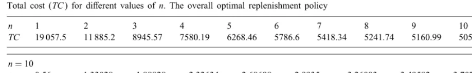
In order to illustrate the preceding theory we consider the following example, which has been used by Hariga and Alyan [13]:
f(t) = 10e0:98t; C= 250; C1= 40; C2= 80; C3= 200; = 0:08; = 0:2; H= 4:
In Table 1, we present the total cost, TC, for dierent values of n and the overall optimal replenishment
policy. The results were obtained using Mathematica. The t∗
1 value was obtained using the Bolzano method
6. Concluding remarks
1. In this model if we set = 0, we obtain the model with complete backlogging developed by Hariga [10].
2. Moreover, taking= 0, = 0 and f(t) linear, we can obtain the model of Goyal et al. [11].
3. The total cost is a decreasing function of the parameter . This implies that the model with this type of
partial backlogging always has smaller total cost than that with complete backlogging.
Appendix A. Checking the conditions for a minimum of TC(n,si,ti).
For convenience let TC(n; si; ti) =TC. To ensure that the solution of Eqs. (9) and (10) gives a minimum,
it is enough to prove that the associated Hessian matrix has positive principal minors. The elements of this Hessian matrix are
The nonzero entries of the Hessian matrix are
H2j+1;2j+1=
Let Mk be the principal minor of order k, then
References
[1] R.E. Bellman, Dynamic Programming, Princeton University Press, Princeton, NJ, 1957.
[2] L. Benkherouf, On an inventory model with deteriorating items and decreasing time-varying demand and shortages, Eur. J. Oper. Res. 86 (1995) 293–299.
[3] T. Chakrabarti, K.S. Chaudhuri, An EOQ model for deteriorating items with a linear trend in demand and shortages in all cycles, Int. J. Prod. Econom. 49 (1997) 205–213.
[4] R.P. Covert, G.C. Philip, An EOQ model for items with Weibull distribution deterioration, Am. Inst. Ind. Eng. Trans. 5 (1973) 323–326.
[5] T.K. Datta, A.K. Pal, Order level inventory system with power demand pattern for items with variables rate of deterioration, Indian J. Pure Appl. Math. 19 (1988) 1043–1053.
[6] U. Dave, L.K. Patel, (T, Si) policy inventory model for deteriorating items with time proportional demand, J. Oper. Res. Soc. 32 (1981) 137–142.
[7] W.A. Donaldson, Inventory replenishment policy for a linear trend in demand: an analytical solution, Oper. Res. Quart. 28 (1977) 663–670.
[8] M.F. Friedman, Inventory lot-size models with general time-dependent demand: an analytical solution, Oper. Res. Quart. 20 (1982) 157–167.
[9] P.M. Ghare, G.F. Shrader, A model for exponentially decaying inventories, J. Ind. Eng. 14 (1963) 238–243.
[10] A. Goswami, K.S. Glaudhuri, An EOQ model for deteriorating items with shortages and a linear trend in demand, J. Oper. Res. Soc. 42 (1991) 1105–1110.
[11] S.K. Goyal, D. Morrin, F. Nebebe, The nite horizon trended inventory replenishment problem with shortages, J. Oper. Res. Soc. 43 (1992) 1173–1178.
[12] M. Hariga, Optimal EOQ models for deteriorating items with time-varying demand, J. Oper. Res. Soc. 47 (1996) 1228–1246. [13] M. Hariga, A. Alyan, A lot sizing heuristic for deteriorating items with shortages in growing and declining markets, Comput. Oper.
Res. 24 (1997) 1075–1083.
[14] R.S. Sachan, On (T, Si) inventory policy model for deteriorating items with time proportional demand, J. Oper. Res. Soc. 35 (1984)
1013–1019.
[15] Y.K. Shah, An order-level lot-size inventory for deteriorating items, Am. Inst. Ind. Eng. Trans. 9 (1977) 108–112.
[16] J.T. Teng, M.C. Chern, H.L. Yang, Y.J. Wang, Deterministic lot size inventory models with shortages and deterioration for uctuating demand, Oper. Res. Lett. 24 (1999) 65–72.
[17] H.M. Wee, Deterministic lot size inventory model for deteriorating items with shortages and a declining market, Comput. Oper. Res. 22 (1995) 345–356.