Vol. 41 (2000) 221–237
Values elicited from open-ended real experiments
John K. Horowitz
∗, K.E. McConnell
Department of Agricultural and Resource Economics, University of Maryland, College Park, MD 20742-5535, USA
Received 20 April 1998; accepted 11 March 1999
Abstract
The idea that preferences are only revealed by real incentives is deeply embedded in economists’ worldview. Consequently, evidence from hypothetical experiments has not readily permeated eco-nomic thinking. One method for determining whether hypothetical experiments provide useful information about preferences is to compare them to similar real-goods experiments.
This study looks at responses elicited by three real experiments. We examine the proportion of responses that meet a series of criteria that range from a broad appeal of plausibility to a narrow re-striction based on quasi-concavity of preferences. We argue that these proportions are unreasonably low. ©2000 Elsevier Science B.V. All rights reserved.
JEL classification: D60
Keywords: Real experiments; Hypothetical experiments; Willingness-to-accept
1. Introduction
Economists frequently conduct experiments in which public or private goods are hypo-thetically traded for money. The responses to these experiments are taken to be motivated by preferences, and so the experiments are useful in learning about preferences and val-uation. For pure public goods, hypothetical experiments such as contingent valuation are sometimes the only way to learn about preferences. The results of hypothetical experiments help determine the policies economists will recommend for environmental amenities and other public goods.
∗Corresponding author. Tel.:
+1-301-405-1273; fax:+1-301-314-9091. E-mail address: [email protected] (J.K. Horowitz).
The idea that preferences are only revealed by real incentives is deeply embedded in economists’ worldview. Consequently, evidence from hypothetical experiments has not readily permeated economic thinking. Students of hypothetical valuation have argued that one method for determining whether these hypothetical experiments provide useful in-formation about preferences is to compare them to similar real experiments in which goods and money are traded in a controlled environment. As real experiments involve real incentives, the argument goes, they provide unimpeachable evidence about prefer-ences. If otherwise similar real and hypothetical experiments yield similar results about preferences, one can conclude that hypothetical experiments provide useful information for policy. The reliability of evidence from real experiments is a critical link in this conclusion.
The role played by real experiments in this link presumes that the ‘realness’ of the experiments, induced by exchanges involving money, elicits preferences. In this paper, we argue that results from a set of real experiments do not conform to what we would expect for real preferences. This raises the question of whether experimental results, real or hypothetical, constitute a useful guide for policy.
Another interpretation of the results relates to the criticisms often applied to contin-gent valuation. Our real experiments show that several kinds of non-economic behavior are exhibited. One can turn this evidence around to argue that when contingent valuation experiments produce odd or non-economic results, the results are not different from what one finds in real experiments, and probably in real social-choice behavior.
The paper approaches the question of the validity of the experimental responses by applying a set of criteria that ranges from a broad appeal of plausibility to a narrow re-striction based on quasi-concavity of preferences. The analysis examines the proportion of respondents from a real experiment that meet each of the criteria. We will argue that these proportions are unreasonably low. We conclude that the link from hypothetical experiments to policy conclusions presumed to be provided by real experiments is weak.
2. Experiments
Three experiments were conducted in-person with small groups. Subjects were endowed either with three pairs of binoculars, three flashlights, or three mugs. The experiments differ from others available in the literature by one or more of the following features: (i) Multiple items of the same good were valued. (ii) The market value of the items was relatively high, especially in the binocular experiment, where the items being valued cost us US$ 75. (iii) The questions were posed as willingness-to-accept (also referred to as compensation demanded, CD) rather than willingness-to-pay. (iv) The subjects were members of the public. (v) A Becker–DeGroot–Marschak (BDM) mechanism with an unspecified range of offer prices was used to elicit compensations demanded.
his compensation demanded. We then repeated the following procedure four times, three times for practice and then for real money and a real transaction. The administrator drew an offer price randomly out of an envelope. If the subject’s compensation demanded was higher than the offer price, the subject kept his mug. If his compensation demanded was less than or equal to the offer price, he returned his mug to us and received a check for the randomly drawn price. All subjects were offered the same offer price. In the flashlight experiment, the subjects were given one mug and three flashlights. In the mug experiment, the subjects were given one flashlight and three mugs. We do not study the values elicited in this first part, which was used to teach the price mechanism to subjects. This mechanism is called a BDM mechanism.
In the second part of the experiment, each subject wrote down two numbers: the minimum payments he/she required to be willing to sell us back two and three binoculars. These are the subject’s compensation demanded for two and three binoculars. We then randomly drew a piece of paper that stated the number of binoculars (per person) we would be buying back. Each option had equal probability, and subjects were told this. For binoculars and mugs, the probability was 1/2 that we would offer to buy back two items and 1/2 to buy back three. For flashlights, the probability was 1/3 that we would offer to buy back one, two, and three items.
We then randomly drew the offer price. For example, we might randomly draw the instruction to buy back two of each subject’s three binoculars, and then draw an offer price of US$ 19.00. This is a price for the two binoculars, not a per-binocular price. All subjects who had offered to sell two binoculars for US$ 19.00 or less then turned in two of their binoculars and received a check for US$ 19.00. They kept their remaining pair of binoculars. All subjects who had offered to sell two binoculars for more than US$ 19.00 kept all three binoculars and received no money.
3. Criteria
We are interested in the values elicited by these experiments. Before one can examine those values, some responses may be deleted for being faulty in one way or another. We set out four criteria to show how the experiments perform under different samples. Some responses are clearly wrong in the sense that one can be reasonably assured that a respondent confronted with his responses would admit they were not his true preferences. Others are wrong for more subtle reasons. The criteria we propose cover a variety of reasons for considering an observation suitable. For each of the experiments, we ask whether the responses meet the following four criteria.
(a) Intuitive plausibility. In the experiments reported, some of the bids are implausible in the sense that almost all observers would agree that they do not represent preferences that any subject would profess to have. In other words, it would seem to be relatively simple to design a comparable experiment in which the subject expressed the opposite preference. These responses have typically been called outliers. For example, one subject reported his CD for two binoculars to be US$ 10 million.
(b) Economic plausibility. When respondents assess their compensation demanded for market goods, they ought to bear in mind the resale value and replacement cost of the goods; in other words, the opportunity costs of otherwise buying or selling the items. Let CDi represent the subject’s compensation demanded to return i items. CDi ought not to exceed the purchase price of those i items, plus transaction cost, because the respondent can replace any or all of his items if offered enough money. CDi ought to exceed resale value because the subject can resell the goods if he gets little utility from having them. Hence, CDiought to be bounded as follows:
Resale value of i items≤CD fori items≤Replacement cost of i items (1)
Economic plausibility requires these bound be met. We put the resale value at zero. (c) The third criterion is based on the marginal compensation demanded rather than total CD. Marginal CD is the extra compensation demanded to give up the ith item, MCD=CDi−CDi−1, with CD0=0.
Marginal CD ought to be higher than the resale value of one item and lower than the replacement cost. Suppose for some non-marketed good, a subject’s CD for two items (when he started with three) was US$ 6 and for three items was US$ 14. Consider what happens if the item could be replaced for US$ 5. The subject’s compensation demanded for three items should now be no more than US$ 11, because for US$ 11, he could buy one of the items and have US$ 6 left over, which gives him the same commodity–money outcome as in the two-item case. Hence, MCD ought to be bounded as follows:
Resale value per item≤Marginal CD≤Replacement cost per item (2)
(c′) Positive marginal value. When the resale value per item is zero, this criterion is identical
to requiring that subjects which have a positive marginal value for the item, MCD > 0. In other words, respondents ought to require more compensation for more goods. When a respondent asks for the same or less compensation for more goods, the criterion fails. This criterion is equivalent to a within-subject test for scale sensitivity in a contingent valuation context.
(c′′) Bounded marginal value. This criterion is the second inequality in expression
(2).
(d) Quasi-concavity of preferences. When multiple items are valued, it is possible to trace out the curvature of the indifference curve between money and the good. If the marginal compensation demanded is increasing in the number of items given up, then the indifference curve would have the usual shape in money and goods. Strictly increasing MCD means that CDi responses are strictly convex in i. Strict convexity is the standard assumption of neoclassical economics. It predicts the pattern (CD1=US$ 2, CD2=US$ 5, CD3=US$ 9) but not (CD1=US$ 4, CD2=US$ 7, CD3=US$ 9). Both patterns meet all of the preceding criteria for a good with replacement cost of US$ 5.
When a subject is asked to report CD for giving up one, two, and three items, as in the flashlight experiment, there are four ways to determine convexity: 2CD3> 3CD2, CD3> 3CD1, CD2> 2CD1, and CD3+CD1> 2CD2. For experiments when subjects report only CD for giving up two and three items, only the first expression can be evaluated. If CDi is strictly convex in i (the standard assumption), each of these expressions will be positive. These tests are not always independent. But if any fails, then the subject has pref-erences that are not strictly quasi-concave. (See Horowitz et al., 1999 for further analysis of convexity.)
Failure of quasi-concavity is different from failure of the other criteria. Respondents can have transitive and believable preferences and be fully exploiting any available opportunity costs, yet still fail quasi-concavity.
For market goods, the bounded marginal value criterion confounds observation of vio-lations of strict quasi-concavity. When replacement cost is US$ 5, a subject might report (CD1=US$ 4, CD2=US$ 9, CD3=US$ 14) even if he had strictly quasi-concave pref-erences; he might have had higher compensation demanded for his third item if a market replacement were not available, but as he can replace his third item on the market, he reports CD3=CD2+replacement cost.
The combined effect of (c′′) and (d) is to allow strictly increasing followed by constant
MCD, everywhere constant MCD, or strictly increasing MCD, when (c′′) is not binding,
but not any other patterns. The combined effect of (c′) and (d) is to reverse these patterns;
in other words, MCD might be constant for a while, then increasing. For example, a subject might report (CD1=US$ 2, CD2=US$ 4, CD3=US$ 8) for a market good whose resale value is US$ 2. In either of these cases, however, MCD should be constant only when it is equal to the resale value or the replacement cost, and in no case will MCD decrease. All of these patterns are accommodated by preferences that are weakly, rather than strictly, quasi-concave.
4. Results
4.1. Binoculars
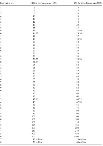
The 48 responses for the binocular experiment are shown in Table 1. The wholesale price for the binoculars was US$ 25 per pair.
(a) Intuitive plausibility. The five highest observations for two binoculars were US$ 250, 300, 1000, 10 million, and 20 million. Designating US$ 10 million and 20 million as implausible is uncontroversial. Decisions about US$ 250, 300, and 1000 are not so easily made. Subject 46, whose CD was US$ 1000, would almost surely have said, in some other context, that he preferred US$ 975 rather than two pair of binoculars, and so we treat his responses as intuitively implausible. We therefore take the three highest responses to be intuitively implausible, leaving 45 observations.
(b) Economic plausibility. Binoculars like the ones used in the experiment cost us US$ 25. We suggest that replacement cost is less than double our cost of US$ 50 for two pairs of binoculars and US$ 75 for three pairs.1 At these payoffs, respondents could easily purchase equivalent binoculars, cover any transactions costs, and pocket some extra money. We designate Observations 39 through 45 as economically implausible. This leaves 38 of the original 48 observations.
(c′) Positive marginal values. A positive marginal value fails if CD2≥CD3, since these
subjects want less than or the same compensation for three binoculars as for two. This rule further eliminates Observations 4, 8, and 22. There are no remaining observations that fail the bounded marginal value criterion. (Observations 39, 40, and 43, which fail the economic plausibility test, also fail to have a positive marginal value.) This leaves 35 of the original 48 observations.
(d) Quasi-concavity of preferences. Of the 35 observations passing the first three tests, 17 have values that are linear in the number of binoculars relinquished, 14 are strictly convex (the typical utility-theoretic prediction), and 4 are strictly concave (nos. 2, 27, 33 and 38). The strict convexity criterion leaves 14 of 48 original observations. The weak convexity criterion leaves 31 of 48 observations.
The two highest CDs conform to standard utility-theoretic predictions as CD3−CD2>
1/2CD2. The US$ 1000 response satisfies this inequality weakly. In other words, the intu-itively implausible responses are well-behaved under this criterion.
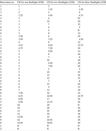
4.2. Flashlights
The flashlight experiment differed from the binocular experiment by: (i) eliciting subjects’ compensation demanded to give up one item of their endowment, as well as two and three items, and (ii) giving subjects an explicit option for declining to give back any flashlights. The 42 responses for flashlights are shown in Table 2.
Table 1
Compensation demanded (CD) for binoculars
Observation no. CD for two binoculars (US$) CD for three binoculars (US$)
Table 2
Compensation demanded for flashlights
Observation no. CD for one flashlight (US$) CD for two flashlights (US$) CD for three flashlights (US$)
1 1 2 1
aSubjects were instructed as follows: ‘If you do not want to sell your flashlights back at any price (you definitely want to keep all three), just put an N in the blank.’
(b) Economic plausibility. We take replacement cost to be less than double our cost of US$ 6.25 per flashlight. Observations 36, 38, 39, and 40 are eliminated this way. This criterion leaves 33 of the 42 original observations.
(c′) Positive marginal values. Subjects can reveal non-positive marginal values if CD1≥
CD2or if CD2≥CD3. Four respondents reveal non-positive marginal values (nos. 1, 12, 22, 37). This criterion leaves 29 observations.
(c′′) Bounded marginal value. Two remaining respondents reveal marginal values for the
third flashlight that exceed the replacement cost bound of US$ 12.50 (nos. 19 and 32). (d) Quasi-concavity of preferences. Of the 27 remaining observations, the strict quasi-concavity criterion leaves two observations (nos. 6 and 7). The weak quasi-quasi-concavity cri-terion leaves 11 observations, the previous two plus seven subjects whose valuations are linear (nos. 4, 8, 13, 14, 23, 31, 35) and two whose valuations are linear then convex (nos. 3, 27).
The flashlight experiment differed in asking for compensation for just one item. This change might be expected to encourage linear responses. However, only seven observations in the 37-observation set are completely linear.
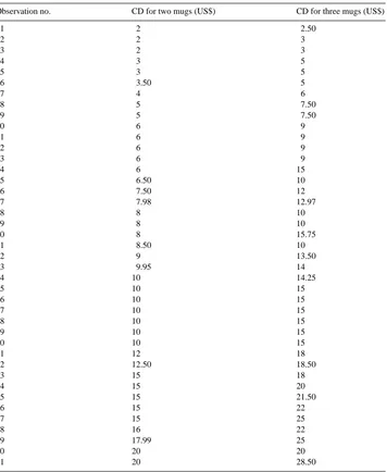
4.3. Mugs
The 41 responses for the mug experiment are shown in Table 3. As in the flashlight experiment, subjects were given an explicit option for declining to give back any mugs.
(a) Intuitive plausibility. The compensation demanded ranged from US$ 2 to 20 for two mugs and from US$ 2.50 to 28.50 for three mugs. The extremes are not obviously implausible. Further, no subject stated he/she would refuse to sell a mug at any price. No observations are excluded for this reason.
(b) Economic plausibility. Mugs like the ones used for this experiment are widely available for around US$ 5–7. We put the replacement cost at just below US$ 8 per mug. Therefore, we view the values revealed by Observations 37 through 41 as economically implausible. This leaves 36 observations of the original 41 observations.
(c′) Positive marginal values. All of the 36 remaining subjects asked more for three mugs
than two. No observations are removed for non-positive marginal values.
(c′′) Bounded marginal value. One subject revealed a marginal value for the third mug
that exceeded the replacement cost bound (no. 14).
(d) Quasi-concavity of preferences. Of the 35 remaining observations, six have values that are strictly convex in the number of mugs relinquished (nos. 4, 5, 15, 16, 17, and 20), and 17 have values that are linear.
5. Analysis
5.1. Effects of criteria on the distribution of values
Table 3
Compensation demanded for mugs
Observation no. CD for two mugs (US$) CD for three mugs (US$)
1 2 2.50
Table 4
Summary statistics for binoculars CD (N=48)
Criterion Mean (US$) Coefficient of Median (US$) Skewness Percent of
variation original
CD for two binoculars a 50.32 1.26 29.00 2.62 94
b 27.36 0.60 21.38 1.04 79
c′
28.27 0.59 22.50 0.95 73
d 26.68 0.53 20.25 0.52 65
CD for three binoculars a 72.63 1.27 45.00 2.88 94
b 41.40 0.58 37.25 0.60 79
c′ 43.66 0.54 40.00 0.52 73
d 42.11 0.50 39.50 0.35 65
Table 5
Summary statistics for flashlights CD (N=42)
Criterion Mean (US$) Coefficient of Median (US$) Skewness Percent of
variation original
CD for one flashlight a 6.19 0.65 5.00 1.54 95
b 5.38 0.52 5.00 0.79 88
c′ 5.38 0.50 5.00 0.78 79
c′′ 5.29 0.49 5.00 0.82 74
d 4.61 0.55 4.00 1.20 26
CD for two flashlights a 10.82 0.67 9.25 1.94 95
b 9.24 0.49 8.50 0.70 88
CD for three flashlights a 16.79 0.67 14.00 1.03 88
b 13.89 0.56 12.00 0.68 79
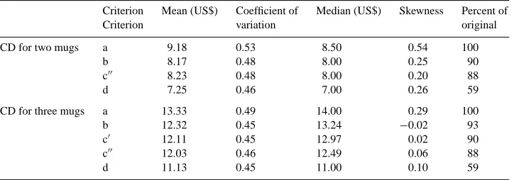
Summary statistics for mugs CD (N=41)
Criterion Mean (US$) Coefficient of Median (US$) Skewness Percent of
Criterion variation original
CD for two mugs a 9.18 0.53 8.50 0.54 100
b 8.17 0.48 8.00 0.25 90
c′′ 8.23 0.48 8.00 0.20 88
d 7.25 0.46 7.00 0.26 59
CD for three mugs a 13.33 0.49 14.00 0.29 100
b 12.32 0.45 13.24 −0.02 93
c′ 12.11 0.45 12.97 0.02 90
c′′ 12.03 0.46 12.49 0.06 88
Table 7
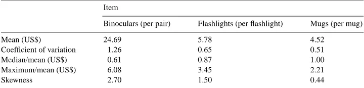
Summary statistics for all observations except outliers Item
Binoculars (per pair) Flashlights (per flashlight) Mugs (per mug)
Mean (US$) 24.69 5.78 4.52
Coefficient of variation 1.26 0.65 0.51
Median/mean (US$) 0.61 0.87 1.00
Maximum/mean (US$) 6.08 3.45 2.21
Skewness 2.70 1.50 0.44
tables the sample statistics are calculated with different samples, labeled (a), (b), (c′), (c′′),
and (d). In Sample (a), the intuitively implausible observations are deleted; in (b), the economically and intuitively implausible are further deleted; in (c′), non-positive marginal
value observations; in (c′′), the observations with too-high marginal values; and in (d),
valuations that are not consistent with weakly quasi-concave preferences.2 We look at the weakest of possible restrictions for Sample (d).
The number of observations that are economically plausible but fail to have positive marginal values and weakly quasi-concave preferences ranges from 14 to 69 percent of the full sample, but the effect of the last two criteria on the central tendency and dispersion of the distributions is mixed. The means change little and the measures of dispersion appear to decline slightly. The main effect of exclusions (c) and (d) is the loss of precision due to the reduction in observations.
5.2. Distribution of values – only outliers removed
Real and hypothetical experimenters commonly analyze responses without appealing to Criteria (b), (c), or (d), either due to the criteria cannot be applied (e.g. only one set of items is valued, which eliminates the marginal value and convexity criteria, or the item is not a private good, which nearly eliminates the economic plausibility criterion) or because the experimenters accept the reported values without applying any judgment. In both of these cases, however, analysts are likely to remove obvious outliers. Table 7 presents statistics from all three experiments with only the intuitively implausible responses deleted.
Lognormal distributions. The lower the mean CD, the smaller the upper tail of the dis-tribution of responses. We find that a lower mean response is accompanied by: (a) a lower standard deviation, relative to the mean, in other words, a lower coefficient of variation, (b) a median closer to the mean, (c) a lower maximum value, relative to the mean, and (d) a lower skewness. These findings are consistent with value distributions that are roughly lognormal, conforming approximately to the shape of a lognormal although not to its range. Number of outliers. The lower the cost of the item, the lower is the number of outliers that are removed.
2For (a) and (b), we remove CDi
Market value and mean CD. When only outliers are removed, mean CDs are remarkably close to the item cost of US$ 25 (binoculars), US$ 6.25 (flashlight), and US$ 4 (mug). A brief look at willingness-to-pay (WTP) experiments shows an analogous pattern. Empirically, mean WTP is roughly half the market price, say 40–60 percent. For example, Loomis et al. (1996) elicited willingness-to-pay for an art print using a first-price auction. Their third treatment, which is the closest to our experiments, found a mean WTP of US$ 14.48, which is 41 percent of the item cost of US$ 35. Johannesson et al. (1997) used a second-price WTP auction for chocolates with 10 participants. The cost was 150 Swedish crowns and the mean WTP was 87.40, which is 58 percent of the price. Neill et al. (1994) conducted a second-price WTP auction for a map. Mean WTP was either 50 or 60 percent of the US$ 20 cost, depending on the treatment of outliers. Horowitz and McConnell (1998) reviewed studies that collected both CD and WTP and found that for ordinary private goods, CD was roughly 2.3 times larger than WTP. If CD is close to market value, then WTP will be 43 percent of market value.3
These results—that mean CD values are close to market value—are striking, but they further indicate how much of the aggregate reported value, roughly half, exceeds the re-placement cost upper bound on CD imposed by economic theory.
6. Interpreting the results
Intuitively implausible responses. By far, the most important decision for analysis is the elimination of implausibly high responses. The effect of outliers is most obvious for the binocular experiment but the effect is also substantial, although the decision less arbitrary, in the flashlight experiments, where five subjects stated that they were unwilling to return some of their flashlights for any offer price. These responses are ones that the subjects themselves would likely admit did not truly reflect their preferences. Low outliers, in which subjects report a value that they would prefer not to accept if it were offered in some other context, may also be present, although they are more difficult to detect and therefore have not been analyzed here.4
We believe the outliers cannot be explained based on the criticism often made of valuation surveys, in general, that the survey places too high cognitive demands on subjects. Subjects might react to our experiment by reporting high values that guaranteed they keep their items, especially, in the binoculars experiment. To guarantee this, a subject needs to guess the highest possible offer price and then state a higher value. (It is not clear that a subject’s guessing the highest offer price places lower cognitive demands than deciding the lowest value he would accept.) A reasonable supposition is that the highest offer price for three binoculars is 1.5 times the highest offer for two binoculars. Responses would follow this pattern as well. Only one of the outliers conformed to this strategy. An alternative response
3Neill et al. (1994) also conducted a second-price WTP auction for an art print. Mean WTP was US$ 9.49, which is 13 percent of the US$ 75 cost, which deviates from the general pattern. Art prints may be too unique to count reliably as ordinary private goods.
strategy is to guess the highest possible offer price over both two and three items and report the same high value for both cases. None of the outliers conformed to this approach.
It is possible that intuitively implausible responses will be a problem only for CD exper-iments, in which subjects are endowed with some item and offered money to return it. CD experiments are much less common than WTP experiments, primarily because response amounts and refusal rates are typically unacceptably high.5 However, if real experiments are therefore unreliable for inferring preferences based on CD, then they cannot be reliable for WTP, since the same economic models are used to motivate and derive lessons from both.
Positive marginal values. The failure for responses to reflect positive marginal values is one of the most unexpected aspects of the experiments. One explanation is that subjects misunderstood the instructions and reported per-item values even though verbal instructions, as well as the written survey, repeatedly emphasized that the subjects should give the total value, not per-item value. A second explanation is that subjects wanted to guarantee the amount of their payment, conditional on receiving payment. This is analogous to the outlier explanation (subjects wanted to guarantee they keep their binoculars), except in the money dimension rather than the goods dimension.
Zero marginal value may occur due to satiation, which seems most likely to happen with mugs. All of the plausible mug responses had positive marginal values.
The anomaly of positive marginal values is akin to a problem in contingent valuation, called insensitivity to scale, in which respondents report approximately the same values for packages of different sizes. A second contingent valuation problem, called insensitivity to scope, arises when subjects report approximately the same values for packages with different attributes; for example, two pairs of binoculars versus two flashlights versus two mugs. In our experiments, responses are clearly sensitive to scope.
Reasonable marginal values. The possibility that marginal values might instead be too high even when the total value is reasonable has not been recognized in the valuation literature. We found one or two subjects who violated this criterion for the mugs and flashlights experiments.
Quasi-concavity of preferences. There is not a clear pattern of failure of quasi-concavity among the experiments. Although a fair number of responses is not neoclassical, their exclusion has little influence on the measures of the central tendency.
7. Related literature
Most of the studies that compare real and hypothetical responses have used closed-ended WTP questions, in which subjects could buy an item (or items) at a given price (Dickie et al., 1987; Cummings et al., 1995, 1997; see also the review in Foster et al., 1997). These studies can provide detailed information about the levels of WTP only when assumptions are made about the underlying value distribution or when both the sample size and the set of offer prices is large. Neither of those remedies is as appealing as an open-ended survey such as the BDM or second-price auction.
A few recent real open-ended studies were discussed in Section 4. The majority of real valuation experiments, however, have been studies of lotteries, which have been examined primarily for their implications about risk attitudes aversion rather than what they actually reveal about values. Much of the recent literature on choice under uncertainty has focused on pairwise choices (e.g. Harless and Camerer, 1994; Hey and Orme, 1994) rather than on open-ended questions.
Most real experiments, including this paper’s, are not fully real but are what might be called ‘randomly real’. In random real experiments, subjects answer several questions, only one of which takes place for real money. In candy bar experiments of Shogren et al. (1994), one out of a subject’s five bids took place for real; in their contaminated sandwich experiments, one out of 20 bids took place. In coke and chocolates experiments of Bateman et al. (1997), one out of 18 bids took place for real. In the experiments reported in this paper, either one out of two or one out of three of a subject’s bids took place for real.
Karni and Safra (1987) show that the BDM mechanism is not everywhere incentive-compatible in eliciting the certainty equivalents of non-degenerate lotteries when subjects have non-expected utility preferences. (See also Holt, 1986 who recognized the role of the independence axiom when only one out of a set of choice experiments is conducted for real, and subjects apply the reduction principle.) The BDM is incentive compatible, however, in eliciting true reservation values for nonrandom bundles, provided only that the subject prefers first stochastic dominance.
The BDM mechanism may, however, not elicit true preferences when subjects anticipate making errors in stating their values. If a subject anticipates making an error, the error introduces an element of risk into the revelation decision. She can reduce this risk by stating a higher mean compensation demanded (i.e. before the error is drawn), since a higher CD reduces the probability that she will return her items and receive the random payment, that is, a higher CD exposes the subject to less risk. If the subject is risk-averse and if she believes that the distribution of price offers has a mean equal to her true mean CD, then she would adopt the strategy of stating a CD that on average is higher than her true value. The size of the bias will be greater the more risk-averse is the individual and the higher is her error variance. Both elements should be small in our experiments. When errors in stated values are possible, the welfare implications of the ‘errors’ themselves are probably much more important than their possible effect on incentive properties and observability.
8. Concluding remarks
Although the values elicited by real valuation experiments are presumably the building blocks of economics, those values have rarely themselves been the subject of analysis. Most studies have compared results across experimental treatments rather than focused on the actual outcomes of a given treatment. This study has looked at the responses that some real experiments elicit.
loose bounds we apply for economic plausibility, many subjects in our real experiments exceeded those bounds, that is, they ignore opportunity costs. We find subjects who appear to ignore either total or marginal opportunity cost. Since opportunity costs are essential to economic logic, their absence in experiments involving real money and real goods (of comparatively high value) casts doubt on the use of real experiments as the sole indica-tors of preferences or as a standard against which hypothetical surveys should be judged. Supporters of real experiments are left with two alternatives.
First, real experiments may be treated as inviolable—researchers can ask positive ques-tions but not apply normative judgments. In other words, the experimenter may be consid-ered to have given up the right to reject any subject’s response in a real experiment, as such a decision runs counter to the claim that these responses are true reflections of value and welfare.
Second, researchers can drop questionable observations and then be satisfied with val-uations from only a portion of the population, perhaps as little as one-half, with the other responses dismissed as either irrational or ‘noisy’ but inconsequential for policy analy-sis. This is analogous to being satisfied with only some experimental procedures, namely, single-item, closed-ended, WTP experiments.
The preferred response, we believe, is to recognize that even the best and most realistic experiments will yield different pictures of ‘preferences.’ Economists should build con-nections between these different expressions of preference. Such an approach should allow both positive and normative exploration of economic behavior.
References
Bateman, I., Munro, A., Rhodes, B., Starmer, C., Sugden, R., 1997. A test of the theory of reference-dependent preferences. Quarterly Journal of Economics 112, 479–505.
Cummings, R., Elliott, S., Harrison, G., Murphy, J., 1997. Are hypothetical referenda incentive compatible?. Journal of Political Economy 105, 609–621.
Cummings, R., Harrison, G., Rutström, E., 1995. Homegrown values and hypothetical surveys: is the dichotomous-choice approach incentive-compatible?. American Economic Review 85, 260–266.
Dickie, M., Fisher, A., Gerking, S., 1987. Market transactions and hypothetical demand data: a comparative study. Journal of the American Statistical Association 82, 69–75.
Foster, V., Bateman, I., Harley, D., 1997. Real and hypothetical willingness-to-pay for environmental preservation: a non-experimental comparison. Journal of Agricultural Economics 48, 123–138.
Harless, D., Camerer, C., 1994. The predictive utility of generalized expected utility theories. Econometrica 62, 1251–1290.
Hey, J., Orme, C., 1994. Investigating generalizations of expected utility theory using experimental data. Econometrica 62, 1291–1326.
Holt, C., 1986. Preference reversals and the independence axiom. American Economic Review 76, 508–515. Horowitz, J.K., McConnell, K.E., 1998. A review of WTA/WTP studies, Unpublished manuscript.
Horowitz, J.K., McConnell, K.E., Quiggin, J., 1999. A test of competing explanations of compensation demanded. Economic inquiry 37, 637–646.
Johannesson, M., Liljas, B., O’Conor, R., 1997. Hypothetical versus real willingness-to-pay: some experimental results. Applied Economics Letters 4, 149–151.
Karni, E., Safra, Z., 1987. Preference reversal and the observability of preferences by experimental methods. Econometrica 55, 675–685.
Neill, H., Cummings, R., Ganderton, P., Harrison, G., McGuckin, T., 1994. Hypothetical surveys and real economic commitments. Land Economics 70, 145–154.