The development of land quality indicators for
soil degradation by water erosion
M.J. Kirkby
a,∗, Y. Le Bissonais
b, T.J. Coulthard
c, J. Daroussin
b, M.D. McMahon
aaSchool of Geography, University of Leeds, Leeds LS2 9JT, UK
bInstitute Nationale pour Recherche Agronomique (INRA) Science du Sol, Avenue de la Pomme de Pin,
B.P. 20 619, Ardon, 45 166 Olivet cedex, France
cInstitute of Geography and Earth Sciences, University of Wales, Aberystwyth, SY23 3DB, UK
Abstract
The paper describes a proposed methodology for estimating water erosion risk for large areas. The estimates are based on a one-dimensional hydrological balance and a physically based sediment transport model. Estimates of risk associated with a given storm amount are integrated over the frequency distribution of daily rainfalls to provide a properly weighted estimate of the average annual risk. Soil factors are estimated from textural classes using qualitative pedo-transfer functions. Climatic data are taken from interpolated gridded data. Topographic data are taken from global or local DEMs. The estimates are for sediment delivery to stream channels. The method has been applied to provide a preliminary estimate for France at a resolution of 250 m, and could be applied globally at a resolution of 1 km. © 2000 Published by Elsevier Science B.V.
Keywords: Soil erosion; Land degradation; Regional modelling; Indicators
1. Introduction
National, European and International agencies need objective information at scales of 1:250,000 to 1:1,000,000 to compare levels of environmental risks, as an aid to economic planning and policy de-velopment. Despite the increasingly effective use of remote sensing, many risk factors are not directly accessible, particularly at this scale. At present, much more can be achieved by combining physically based models with remotely sensed land cover, digital ele-vation models, gridded climate data and databases of fixed soil and other characteristics. Early versions of one such proposed modelling approach are currently
∗Corresponding author. Tel.:+44-113-233-3310;
fax:+44-113-233-6758.
E-mail address: [email protected] (M.J. Kirkby).
being implemented within EU Environment projects — MEDALUS and MoDeM — in close co-operation with the Space Applications Institute of European Joint Research Centre (JRC), Ispra, among others. A preliminary erosion risk map of France is also be-ing prepared, in collaboration with JRC and Institute Nationale pour Recherches Agronomiques (INRA), Orléans, for comparison with CORINE methods (Briggs and Giordiano, 1992), and these methods are now being improved and taken forward in ongoing work.
The objective of this work is to provide indicators of soil erosion risk at a regional scale, which are suit-able for planning and policy for national to continental areas. Although risk is at present expressed on a quali-tative scale, the values are closely related to estimated average rates of water erosion, calculated month by month. Because of the uncertainties of the weather,
these values cannot be regarded as forecasts, but are a weighted average based on the expected long-term frequency of storms of all magnitudes.
2. Method
The proposed physical model is based on a one-dimensional soil-vegetation-atmosphere transfer (SVAT) type scheme for surface hydrology, coupled where appropriate to a dynamic model for generic vegetation growth, controlled by available water, po-tential evapotranspiration and temperature. It has been developed from a basis in earlier work (de Ploey et al., 1991; Kirkby, 1994; Kirkby and Cox, 1995) on soil erosion. These variables are among the critical and dynamic controls for a many earth surface processes. The methodology may be applied to a number of environmental processes. At present it is being ap-plied to water erosion, salinisation, depth of the ac-tive (unfrozen) layer and peat mire accumulation. It is also proposed to extend it to wind erosion in the near future.
Water erosion is directly controlled by
1. Climate — through the distribution of storm events 2. Vegetation — via crown cover, providing protec-tion from rainsplash impact and via root mat strength
3. Soil properties — texture, organic matter and struc-ture influence both water storage and resistance to sediment detachment and transport (erodibility) 4. Topography — through hillslope length
(repre-senting the collecting area for overland flow) and through gradient (as the driver for sediment traction)
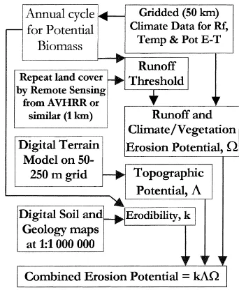
A number of these factors act through agricultural land use, which is itself influenced by economic and social factors (Fig. 1).
2.1. Scientific rationale for estimating erosion risk
The combined erosion index (Fig. 2) is obtained as an estimate of mean soil loss in tonne ha−1, as a prod-uct of terms which are primarily dependent on soil, cli-mate/vegetation and topography, integrating over the frequency distribution for each month to give
Y = p2kR2r0Rexp
−h
r0
H2exp(−2/r0H )
L . (1)
Fig. 1. Factors influencing water erosion rates.
where Y is the sediment loss, R the total monthly rain-fall, r0the mean rain per rain-day, h the runoff thresh-old, p the proportion of runoff above threshthresh-old,Θthe tractive stress threshold, k the soil erodibility, H the mean slope relief and L the mean slope length.
Daily rainfall intensity is represented above by a simple exponential distribution above. Better fits may be obtained using the sum of two exponential curves, or the more general Gamma distribution, as is indicated below. Such an expression makes use of widespread daily rainfall data. This cannot reflect
detailed differences in storm intensity profiles, but does contain information about the frequency distri-bution of daily rainfalls, represented by the mean rain per rain-day (r0) above, and by its standard deviation in Eqs. (9) and (10) below. Over the frequency dis-tribution, Eq. (1) gives due weighting to the greater impact of large flows, and the dominant event size for erosion can be derived (de Ploey et al., 1991) as a daily rainfall of r0+2h, which has a recurrence interval of 1/N0exp (1+2h/r0) years.
2.1.1. Runoff threshold
A one-dimensional dynamic model for hydrology is based on 50 km or less gridded climate data, as average monthly values, historic sequences or fu-ture GCM-based scenarios. Monthly values can be used to grow potential ‘natural’ vegetation and soil organic matter within the SVAT, to provide crop states for each specified land use, or, in combination with a socio-economic model, to forecast land use in response to climatic and economic factors.
Forecast values can be compared with, or replaced by monthly land cover maps derived from AVHRR satellite mosaics, using corrected NDVI and surface temperature estimates. Differences between cover ob-tained from these two approaches provide one impor-tant and direct index of change.
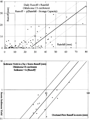
The runoff threshold and proportion of subsequent runoff are simplifications of cumulative infiltration and runoff curves, illustrated in Fig. 3 for a USDA experimental catchment in Oklahoma for which data is available. Runoff Threshold is generally estimated from the crown cover, soil organic matter and soil texture/structure characteristics, since data like that of Fig. 3 is not widely available. It may be seen that this relationship shows a large amount of scatter, and this is typical of such data. The large amount of scatter around the threshold point is readily understood in terms of the (generally unknown) variations in rainfall intensity combined within the simplified relationship, as can be seen when comparable theoretical curves are generated from a semi-empirical infiltration ex-pression such as the Green-Ampt or Philip equation. The threshold represents the effects of surface storage in random roughness and plough furrows, the dy-namic evolution of soil crusting and moisture storage within the upper soil layers. Surface storage changes rapidly over the year on cultivated land, as raindrop
impact crusts newly ploughed land, and reduces fur-row roughness, and this is one source of the scatter shown in a single grouped plot like that of Fig. 3a.
The runoff model, for a daily rainfall of r, is then used in the simple form:
j =p(r−h) (2)
q=xj
where j is daily runoff and q the overland flow dis-charge (per unit flow strip width)
This relationship is recognised as a simplification which neglects the variations in rainfall intensity in the course of a storm, and the duration of bursts of intense rainfall during which runoff accumulates downslope. Work is in progress on improving these approxima-tions in Eq. (2). Preliminary results indicate that dis-charge increases less than linearly downslope, and that an equilibrium discharge is reached after a distance which increases with mean intensity.
2.1.2. Erodibility and traction thresholds
These depend on soil and vegetation characteris-tics. As vegetation cover changes in a given rainfall regime, sediment loss is directly related to runoff, as illustrated in Fig. 4 for loess soils in Mississippi. High traction thresholds are usually associated with strong grass or tree root mats and/or very stony soils. This approach, linked to studies of fluvial sediment trans-port, appears to be generally applicable to overland flow, as indicated by small scale flume experiments, but relies on locally relevant parameter values for soil and land cover combinations.
2.1.3. Topographic factors
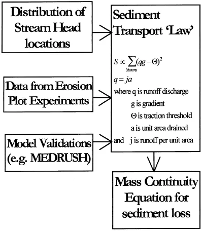
Topographic factors in the sediment loss equation are chosen to be consistent (Fig. 5) with data from the long-term erosional forms of hillslope profiles, with the location of stream heads which evolve over pe-riods of 10s to 100s of years (Dietrich and Dunne, 1993; Poesen et al., 1997), and with erosion plot ex-periments over 1–20 years, including data sets such as that shown in Fig. 4. This approach provides a robust formulation for a wide range of current and possible changed conditions.
Fig. 3. Runoff and Sediment Yield for USDA Catchment C5, Oklahoma (from Kirkby, 1998). (a) Overland flow runoff vs. storm rainfall. (b) Sediment yield vs. overland flow runoff in each storm.
analysis of the forms requires assumptions, not gen-erally justified in detail, that the landform is either declining exponentially towards a base level (Kirkby, 1971) or that it is being lowered at a uniform rate (Hack, 1960), perhaps in balance with tectonic up-lift. The latter assumption is simpler to implement. If the slope profile is expressed in a functional form, then possible sediment transport expressions are con-strained as follows:
For a slope profile form z=f(x) and a sediment transport law assumed to be of form S=φ(x)gn, the
expressionφ(x) is constrained to the form:
φ (x)=Tx[f′(x)]−n (3)
where x is distance downslope, z the elevation, g the local slope gradient, T the constant rate of denudation and the′ indicates differentiation.
Fig. 4. The relationship between sediment yield, runoff and vegetation type, holly springs, Mississippi (data from Meginnis, 1935 in Kirkby, 1998).
For a long-term sediment transport law of the form:
S=κhg+x u
xg u −θ
i
(4)
for constants κ, u and θ is associated with the convexo–concave slope form:
Fig. 5. Sources of data for sediment transport dependence on topography.
z=u 2
Tu
k +θ
"
ln 1+x 2 0 u2
!
−ln
1+x 2 u2
#
where x0is the slope length.
In some areas with a relatively unchanging climate, these methods are in accord with cosmogenic dating, although this accordance is not expected in areas of actively accelerated soil erosion.
The position of stream heads in permanent channels and ephemeral gullies give the best data for Traction thresholds. Valleys grow where there is positive feed-back which concentrates erosion, giving a downslope zone of unstable growth, where:
x∂S
dx > S in general (5)
and for the sediment transport law in Eq. (4),
x > u
Erosion plot data provides some systematic informa-tion on the effect of individual storms, which may be represented by a disaggregated form of Eq. (4), roughly replacing distance by discharge as:
S∗=κ′
g+ q q∗
qg
q∗ −θ ′
(6)
A form of this kind can be formally re-aggregated to a long term relationship through integration over the frequency distribution of storm flows.
These three types of data on transport rates are all consistent with the proposed form, which is there-fore known to respond robustly across a range of time scales. The form presently adopted is:
At the storm level:
S∗=κgr2+µ(qg−θ )2 where r is the storm rainfall.
If integrated over an exponential rainfall frequency distribution, the long-term equivalent is:
S=2p2Rr0 mean rain per rain-day.
In the erosion risk model, these effects of topogra-phy are integrated through local hillslope relief, which is obtained from 50 to 800 m DEM grids as the stan-dard deviation of elevation within a 1 km radius of each point. This measure is both relevant to the model and stable over a range of DEM resolutions. Relief, H, obtained in this way is a good estimate of the term xg which appears in Eq. (7). Similarly slope length, L, may be estimated from the frequency of gradi-ent reversals on high quality DEMs, but is generally considered to be a more conservative parameter than relief. Ignoring the small first term in Eq. (7), the total estimated sediment loss delivered to the slope base is:
Y = S
The final terms, in H and L, are the topographic com-ponents of the erosion indicator. It should, however, be noted that relief is inversely related to soil erodibil-ity through lithology and texture, so that a relief factor must be combined with good soil type data.
2.1.4. Potential natural vegetation model
In most applications it is preferable to derive land cover directly from existing maps (such as CORINE land cover), or up-dateable remote sensing methods, such as those based on AVHRR for 1 km resolution.
It is, however, sometimes useful to compare these ‘actual’ cover distributions with the ‘potential’ vege-tation, based on climatic and other environmental con-straints alone. The proposed vegetation growth model for this purpose is a dynamic carbon balance model, responding to monthly actual evapo-transpiration us-ing a water use efficiency (WUE) approach. Vegeta-tion is generic, but a survival model for cover gives some indication of morphology. The budget provides a simultaneous estimate of SOM, which is an impor-tant variable in forecasting the runoff threshold.
Differences between computed potential unculti-vated vegetation and remotely sensed or surveyed actual land cover give a direct measure of total human disturbance. Agricultural landuse may, in this scheme, also be simulated directly by removing cropped ma-terial from the budget at harvest time, in a way which reflects farming practice interacting with inter-annual variability. Over a restricted climatic range, this may be related to a fixed cultivation timetable, but a more generic approach is to relate harvest-time to the pe-riod of maximum biomass. Material harvested not only limits further growth, but also intervenes in the transfer of leaf-fall from plant to soil organic matter.
2.1.5. Frequency distribution of erosive storms Summation over storms is better achieved by fitting the distribution of daily rain amounts to a sum of two exponential distributions rather than a single exponen-tial as used for illustrative purposes above, using the monthly values for number of rain days, mean rain-day and its standard deviation. Thus, the frequency den-sity, N(r), for a daily rainfall in excess of r is
N (r)=N0
whereµis a fraction, normally between 0 and 1, N0 the total frequency of rain-days=N(0), and r1,r2 are rainfall intensity parameters.
The mean and variance of this distribution are:
¯
r=µr1+(1−µ)r2
Integration of the storm runoff and sediment trans-port equations can be carried out analytically over this distribution to give the form of the erosion risk ex-pression. The overall effectiveness of the erosion risk estimates may be compared with observed empirical relationships between sediment loss and climate, with a minimum in temperate zones. A model compari-son (Kirkby, 1995) with a transect across the southern United States shows fair qualitative agreement with empirical summaries (Langbein and Schumm, 1958).
3. Results and discussion
3.1. Applications to erosion risk in France
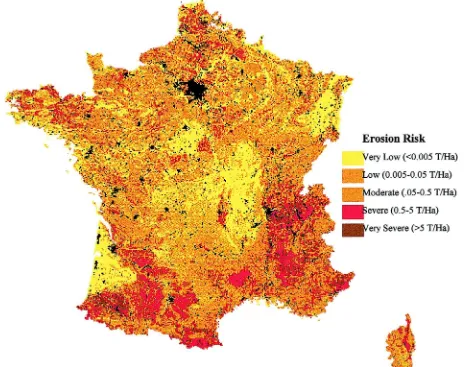
A preliminary attempt has been made to imple-ment these methods for France, based on data held by INRA, Orléans, and which has already been used to prepare a preliminary qualitative assessment (Montier et al., 1998). Parameters have been derived from the CORINE land cover survey, a 5 km gridded database for interpolated monthly mean rainfall totals, a 250 m resolution DEM and information from the draft Eu-ropean Geographic Soils Database. These have been used to create qualitative pedo-transfer functions, based primarily on INRA experience, to estimate monthly vegetation cover, runoff thresholds, crusting class and soil erodibility. A preliminary map, show-ing the feasibility of the approach, is shown in Fig. 6 (Yassoglou and Jones, 1998; Kirkby et al., 1998), but the results are, to date, not fully validated.
This exercise demonstrates that these methods are able to lead to reasonable estimates of monthly average erosion rates, but that there is considerable scope for improvement in parameterisation from existing data sources, the creation of additional special purpose data layers within European Databases, and for a substan-tial exercise in validation at a range of appropriate scales.
This work has been completed, using the meth-ods set out above, generating monthly and annual estimates of erosion risk. These are presented in cat-egories, which are provisionally classified as mean erosion loss rates. At present pedo-transfer rules have been based on the experience of Le Bissonais and other colleagues at INRA, Orléans, but the final product is un-validated at this stage. Although the
resolution shown is 250 m, it should also be recog-nised that less reliance should be made on individual pixel values than on the clear regional patterns. Fore-casts are available for each month, and could also be expressed in terms of the probability of exceedance of a given event size.
3.2. Data sources
3.2.1. Soils
The European Geographic Soils Database for France is clearly the best and main source for erodi-bility and some of the soil storage terms. Following the results of Montier et al. (1998) and Le Bissonais et al. (1996), the values were used for the trial run based on data in the European Soils Database (Tables 1–3).
3.2.2. Land cover
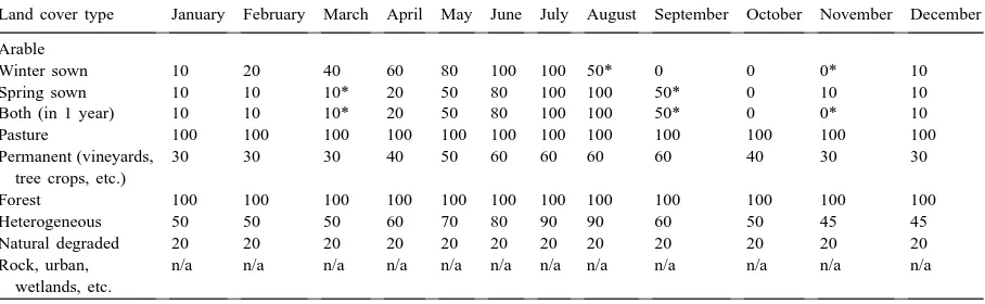
The CORINE land cover map has been used. Stan-dard functional conversions were used to convert cover types to vegetation cover % (Table 4).
Land cover classes were taken from the CORINE database. Additional information for types of arable farming were taken from the table of Petits Régions Agricoles (PRA) crop returns for the same year, linked
Table 1
Erodibility classes from categories in European soils database Relative
Moderate 3 Moderate ±50
Strong 10 Strong ±20
aThe relative erodibility class is taken directly from the pedo-transfer functions in Montier et al., 1998.
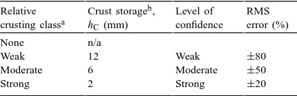
Table 2
Crusting classes from categories in European soils database Relative
crusting classa
Crust storageb,
hC(mm)
Weak 12 Weak ±80
Moderate 6 Moderate ±50
Strong 2 Strong ±20
aThe relative crusting class was taken directly from the classes (‘Battance’) in Montier et al., 1998.
Fig. 6. Preliminary erosion risk map of France, at 250 m resolution.
Table 3
Water retention estimates from categories in European soils database Soil texture classa Water retention (mm)
at saturation
Water retention (mm) at field capacity (50 cm)
Soil storage,
hS(mm)
Coarse 403 294 109
Medium 439 379 60
Medium fine 430 406 24
Fine 520 472 48
Very fine 614 567 47
Organic soils 766 708 58
Table 4
Land cover types from CORINE classification in ESDB Land
cover typea
Initial surface storage, hR, (mm)
Reduction per month (%)
Arable 10 50
Other 5 0
aLand cover type was also taken from the CORINE database. Arable storage was set to its initial value at times of cultivation (taken as seed-time and harvest).
Table 5
Interception (as percentage of storm rainfall) estimated from ESDB Land cover type Interception storage, hI,
as % of storm rainfall
Arable 5
Pasture, vineyards and tree crops 10
Forest 20
Heterogeneous 10
Natural degraded land 5 Urban, rock, wetlands n/a
to the database layer which identifies the PRA of each cell. This gave the proportions of winter and spring sown arable, together with a total arable. If there were areas with both categories of arable, subtraction gave an estimate of the area with both types in the same year. This provided estimates of initial surface storage (Table 4), interception (Table 5) and vegetation cover for each month of the year (Table 6).
3.2.3. Topography
Relief was estimated as the standard deviation of re-lief at each point in a DEM, based on all points within
Table 6
Land cover type from CORINE database within ESDB
Land cover type January February March April May June July August September October November December Arable
Winter sown 10 20 40 60 80 100 100 50* 0 0 0* 10
Spring sown 10 10 10* 20 50 80 100 100 50* 0 10 10
Both (in 1 year) 10 10 10* 20 50 80 100 100 50* 0 0* 10
Pasture 100 100 100 100 100 100 100 100 100 100 100 100
Permanent (vineyards, tree crops, etc.)
30 30 30 40 50 60 60 60 60 40 30 30
Forest 100 100 100 100 100 100 100 100 100 100 100 100
Heterogeneous 50 50 50 60 70 80 90 90 60 50 45 45
Natural degraded 20 20 20 20 20 20 20 20 20 20 20 20
Rock, urban, wetlands, etc.
n/a n/a n/a n/a n/a n/a n/a n/a n/a n/a n/a n/a
a given radius. Test show that this is not sensitive to the DEM resolution, although the radius used is limited to requiring at least five points in the sample (i.e mini-mum radius≥DEM cell size). A radius of 1 km worked well, and was satisfactory using the 250 m DEM for France available, with permission, through INRA.
3.2.4. Climate
The 5 km interpolated rainfall map for France gave an excellent quality for monthly mean rainfalls. In addition the table for≈90 stations in France gave the frequency of 24 h totals which were used to obtain the frequency distribution of daily rainfalls. Values of the mean rain per rain day and its standard deviation were then assigned back to the 5 km grid to fit the distributions of monthly rainfall intensities.
3.2.5. List of data required
All of these are held by INRA for France, and are subject to permission for use in the proposed context (Table 7). They comprise a series of data layers from the soils database at 250 m resolution, monthly pre-cipitation at 5 km resolution, additional tables of Pe-tits regions Agricoles (PRA) and station climatic data. These data are then processed using a series of Arc Macro Language (AML) algorithms.
3.3. Comparison with the INRA erosion risk map of France
Table 7
Data required for LQI erosion model
Layers in soil database at 250 m resolution
1. Erodibility classes and reliability (2 layers) 2. Crusting classes and reliability (2 layers) 3. Soil texture classes
4. CORINE land use classes 5. PRA membership 6. Elevation (DEM/MNT)
7. Slope classes (for comparison only)
Data layers at 5 km resolution
Monthly mean precipitation (12 layers)
Tables
1. PRA: Partition between crop classes (esp. winter and spring sown arable)
2. Climate data for 90 stations. Distribution of intensities for 24 h rainfall (by month if available)
Algorithm/Program
Interpolation routine used to apply metro station data to 5 km grid. The complete set of rules and algorithms was applied through macros (AML) in Arc-Info to obtain the final maps for average erosion risk in each month, as an estimated mean erosional loss. The annual map is the sum of the 12 months
local and regional convergence with the INRA maps, but there are also divergences. For example, the Laura-gais SE of Toulouse is well known for erosion prob-lems, which are better identified in the RDI than in the INRA map. However, in other areas the RDI model seems to overestimate erosion, such as in central Bre-tagne, between Rennes and Nantes, in Basse Nor-mandie between Caen and Granville, and in the Jura area along the Swiss border. Many of these areas are almost completely covered by vegetation, grassland and forest, respectively. In the initial runs, the whole of south and east France generally also showed too high an erosion rate, and this contrast has been reduced by modifying the relief factor in the RDI estimator. It is planned to improve and validate the model properly within a Framework V research grant (PESERA).
4. Conclusions
There is a lot of fine-tuning to do with the model before it is satisfactory, particularly for the whole of Europe, but the quantitative RDI model has the po-tential for dealing with it, probably more easily than the expert based model, and forms a basis which is capable of replacing the CORINE estimates for the whole of Europe, without making excessive data de-mands. Further development is, however, essential, before the results can be considered reliable, and
there may be minor difficulties with available data at a sufficiently high spatial resolution. To produce an erosion risk map at 250 m or 1 km resolution would currently be constrained to some extent by the quality of DEMs (currently 5′′ or 1 km) and of interpolated climate data (currently 50 km in the MARS database), but other variables are sufficiently described in the EGSDB for soils and the CORINE system for land use, although the latter might well be superseded by sequential AVHRR or Spot Végétation monthly cover. It is an important feature of the RDI estimates that they are not strongly dependent on the pre-cise data specification, and can be adapted to make use of the best available data for each part of the area.
This paper outlines a scientifically consistent and objective approach to regional indicators for land qual-ity or land degradation. A similar methodology can be applied for a number of other land quality and risk factors, to provide maps and databases at scales of 1:1,000,000, but each requires research, and is far from a simple compilation exercise. Example factors for which preliminary work has started include soil salinisation, the distribution of peat mires, depth of the active layer in cold climates, mass movements and wind erosion.
and to allocate resources for more detailed investi-gation.
The nature of regional indicators is that they pro-vide only a general overview. Coarse scale indicators should be used to define areas where more detailed studies are needed. They are therefore seen as the outermost shell for an explicitly nested approach to determining and mitigating risks. As the scale changes, the dominant controlling factors also change, from climatic and macro-economic at continental scales, to considerations of local topography, aspect and individual farming practice at the scale of a community at which remediation strategies must be applied.
The scientific rationales at these widely different scales should remain compatible. In this way pa-rameters of regional indicator model may be derived from and related to more detailed catchment or plot models.
Acknowledgements
The research reported in this paper has been largely supported by the European Commission through the MEDALUS III (DGXII, Environment and Climate) and MODEM (DG JRC, Ispra) projects. The work on France has been done in close collaboration with staff at INRA, Orléans, supported by a small contract from the European Soils Bureau.
References
Le Bissonais, Y., Benkhadra, H., Chaplot, V., Gallien, E., Eimberck, M., Fox, D., Martin, P., Ligneau, L., Ouvry, J.F., 1996. Genèse de ruissellement et de l’érosion diffuse des sols limoneux: analyse du transfert d’échelle du m2 au versant. Géomorphologie: relief, Processus, Environment 3, 51–64.
Briggs, D., Giordiano, A., 1992. CORINE soil erosion risk and important land resources in the southern regions of the European Community E.C., Luxembourg, 97 pp.
Dietrich, W.E., Dunne, T., 1993. The channel head. In: Beven, K., Kirkby, M.J. (Eds.), Channel Network Hydrology. Wiley, London, pp. 175–219.
Hack, J.T., 1960. Interpretation of erosional topography in humid temperate regions. Am. J. Sci. 258A, 80–97.
Kirkby, M.J., 1971. Hillslope process-response models based on the continuity equation. Trans. IBG Special Publication 3, 15– 30.
Kirkby, M.J., 1994. Thresholds and instability in stream head hollows: a model of magnitude and frequency for wash processes. In: Kirkby, M.J. (Ed.), Process Models and Theore-tical Geomorphology. Wiley, London, pp. 295–352.
Kirkby, M.J., 1995. Modelling the links between vegetation and landforms. Geomorphology 13, 319–335.
Kirkby, M.J., 1998. Evaluation of plot runoff and erosion forecasts using the CSEP and MEDRUSH models. In: Boardman, J., Favis-Mortlock, D. (Eds.), Modelling Soil Erosion by Water. Springer, Berlin, pp. 33–42
Kirkby, M.J., le Bissonais, Y., Daroussin, J., King, D., 1998. A provisional erosion risk map of France using a new Pan– European Approach. Report on contract to the European Soil Bureau, Joint Research Centre (unpublished).
Kirkby, M.J., Cox, N.J., 1995. A climatic index for soil erosion potential (CSEP) including seasonal and vegetation factors. Catena 25, 333–352.
Langbein, W.B., Schumm, S.A., 1958. Yield of sediment in relation to mean annual precipitation. Am. Geophysical Union, Trans. 39, 1076–1084.
Meginnis, H.G., 1935. Effect of cover on surface runoff and erosion in the Loessial Uplands of Mississippi. U.S. Department of Agriculture Circular 347, 15 pp.
Montier, C., Le Bissonais, Y., Daroussin J., King, D. Draft report 1998. Cartographie de l’Aléa Erosion des Sols en France. INRA, Orléans: Draft Report.
de Ploey, J., Kirkby, M.J., Ahnert, F., 1991. Hillslope erosion by rainstorms — a magnitude-frequency analysis. Earth Surface Processes Landforms 16, 399–409.
Poesen, J., Oostwoud Wijdenes, D., Vandekerckhove, L, 1997. MEDALUS III Project 4: Ephemeral Channels and Rivers, Fourth Interim Report, pp. 3–9.