A comparison of two statistical methods for spatial interpolation of
Canadian monthly mean climate data
David T. Price
a,∗, Daniel W. McKenney
b,1, Ian A. Nalder
c,2,
Michael F. Hutchinson
d,3, Jennifer L. Kesteven
d,3aCanadian Forest Service, Northern Forestry Centre, 5320-122 Street, Edmonton, Alta., Canada T6H 3S5 bCanadian Forest Service, Great Lakes Forestry Centre, 1219 Queen Street East, Sault Ste. Marie, Ont., Canada P6A 5M7
cDepartment of Renewable Resources, Faculty of Agriculture, Forestry and Economics, University of Alberta,
Edmonton, Alta., Canada T6G 2E3
dCentre for Resource and Environmental Studies, The Australian National University, Canberra ACT 0200, Australia
Received 11 August 1999; received in revised form 8 December 1999; accepted 9 December 1999
Abstract
Two methods for elevation-dependent spatial interpolation of climatic data from sparse weather station networks were compared. Thirty-year monthly mean minimum and maximum temperature and precipitation data from regions in western and eastern Canada were interpolated using thin-plate smoothing splines (ANUSPLIN) and a statistical method termed ‘Gradient plus Inverse-Distance-Squared’ (GIDS). Data were withheld from approximately 50 stations in each region and both methods were then used to predict the monthly mean values for each climatic variable at those locations. The comparison revealed lower root mean square error (RMSE) for ANUSPLIN in 70 out of 72 months (three variables for 12 months for both regions). Higher RMSE for GIDS was caused by more frequent occurrence of extreme errors. This result had important implications for surfaces generated using the two methods. Both interpolators performed best in the eastern (Ontario/Québec) region where topographic and climatic gradients are smoother, whereas predicting precipitation in the west (British Columbia/Alberta) was most difficult. In the latter case, ANUSPLIN clearly produced better results for most months. GIDS has certain advantages in being easy to implement and understand, hence providing a useful baseline to compare with more sophisticated methods. The significance of the errors for any method should be considered in light of the planned applications (e.g., in extensive, uniform terrain with low relief, differences may not be important). ©2000 Elsevier Science B.V. All rights reserved.
Keywords:Climate; Temperature; Precipitation; Spatial interpolation; Topographic dependence; Canada; Thin-plate smoothing spline; ANUSPLIN; GIDS
∗Corresponding author. Tel.:+1-780-435-7249; fax:+1-780-435-7359.
E-mail addresses:[email protected] (D.T. Price), [email protected] (D.W. McKenney), [email protected] (I.A. Nalder), [email protected] (M.F. Hutchinson), [email protected] (J.L. Kesteven).
1Tel.:+1-705-759-5740; fax:+1-705-759-5700. 2Currently resident in Australia. Tel.:+61-2-6254-3322. 3Tel.:+61-2-6249-4783; Fax:+61-2-6249-0757.
1. Introduction
The development of methods to interpolate climatic data from sparse networks of stations has been a fo-cus of research for much of this century (Thiessen, 1911; Shepard, 1968; Hughes, 1982; Hutchinson and Bischof, 1983; Phillips et al., 1992; Daly, 1994). Re-cent events, including the IPCC Second Assessment
Report on climate change (Houghton et al., 1996) and the Kyoto Protocol of late 1997, have sparked additional interest in climate data interpolation. Pre-diction of the impacts of a changing climate on the distribution and functioning of terrestrial ecosystems requires as a first step, the development of reliable, spatially-explicit models of current climate. For many of the areas of greatest concern, such as the boreal forest and tundra biomes of central and northern Canada, station coverage is often very sparse, and the long-term records often incomplete. In addition, many researchers attempt to predict future ecosys-tem responses to climatic change using output from general circulation models (GCMs) and regional climate models (RCMs) (Boer et al., 1992; Caya et al., 1995). Although there are undoubtedly many conceptual problems and practical limitations to us-ing coarse-scale climate model output for predictus-ing ecosystem responses, any attempt to do this will gen-erally require an unbiased method for interpolation to the scale of operation of most ecosystem models. Im-proved methods of climate interpolation will enhance our ability both to quantify effects of climate (and cli-mate variability) on natural and managed ecosystems, including forests, wetlands and agroecosystems, and to forecast the possible impacts of climate change. In most cases, simulation of ecosystem responses to climate does not require an exact representation of reality, so interpolation from sparse or incomplete records is quite acceptable. However, because many natural vegetation types occur in mountainous re-gions, it is reasonable to suppose that elevation is a key factor influencing the climate experienced by these ecosystems. Hence it is generally necessary to include elevation as an independent variable in the interpolation method.
In some instances, it may be preferable to use a simple method applied to the region of interest than to use a more sophisticated approach which could be marginally more accurate, but requires considerably more time and money to implement. In this paper, therefore, two elevation-dependent climate interpolators are compared. One of these, ANUSPLIN (Hutchinson, 1995a, 1999), has been developed and tested over several years and is now widely used. The other interpolator, Gradient plus Inverse-Distance-Squared (GIDS) (Nalder and Wein, 1998), is less well known but attractively simple
and appears to give results adequate for modelling forest ecosystem responses to climate — at least in relatively flat terrain.
Recently, Price et al. (1998) generated national-scale gridded climate surfaces for Canada using the GIDS weighting method of Nalder and Wein (1998). Nalder and Wein (2000, in press) developed GIDS as a straightforward method for interpolating cli-mate data obtained from a sparse regional net-work of stations in northwestern Canada to the positions of a large number of survey plots lo-cated in boreal forest stands. Using multiple lin-ear regression to estimate regional gradients in temperature and precipitation with latitude, longi-tude and elevation, GIDS was found to compare very favourably with several other interpolation methods, including universal kriging, while having the benefit of straightforward implementation and operation.
McKenney et al. (2000, submitted for publication) have also developed national climatic grids, expand-ing on previous work in Ontario and the Great Lakes (Mackey et al., 1996) using the ANUSPLIN soft-ware of Hutchinson (1999) (see also Hutchinson, 1991, 1995a; Hutchinson and Gessler, 1994). ANUS-PLIN is based on smoothing splines as described by Wahba (1990), Hutchinson (1984) and Wahba and Wendelberger (1980). Additional FORTRAN pro-grams in the ANUSPLIN modeling package can be used to generate interpolated grids and, hence, dig-ital climate maps. In this paper, we compare GIDS with ANUSPLIN through a data-withholding pro-cess and attempt to identify the ‘better’ approach to generating digital grids of monthly mean climate for Canada.
per-sonal communication, 1999, Canadian Forest Service, Edmonton).
2. Methods
2.1. GIDS
GIDS relies on multiple linear regression (MLR) analysis of data from a set of nearby stations to
esti-Vp=
mate the local gradients for each climate variable, treating latitude, longitude and elevation as inde-pendent variables. The climate value for a target point in the neighbourhood is then predicted from the same station data, using the MLR coefficients to correct for the differences from each station’s posi-tion. The contributions of each station to the final estimate are inverse-weighted by their squared dis-tances to the target point, i.e., GIDS assumes that climate data are spatially autocorrelated. Clearly, there are some important caveats to this assumption, particularly in mountainous regions where topog-raphy tends to reduce spatial correlations (at least when considering two dimensional space) and thus affects the predictability of both temperature and precipitation.
Following Nalder and Wein (1998), computer programs were written to perform MLRs for each monthly climate variable at the location of every test station or grid point, using routines for the matrix solution of linear equations from Press et al. (1986). The solutions yielded sets of coefficientsCX,CY and CZ, representing the observed gradients of variableV
in response to independent variables X,Y, Z, denot-ing longitude, latitude and elevation asl, respectively. To account for the effect of possible non-linearities associated with convergence of the meridians at high latitudes, differences in spherical coordinates between the target location and the neighbouring stations were also mapped on to planar distance
co-ordinates using an Azimuthal Equidistant projection algorithm given in Snyder (1987). In practice, this transformation was found to have negligible impacts on the average R2 of the MLRs and was not used further.
The MLR coefficients were then used to predict each climate variable,Vp, at each target climate sta-tion, from the coordinates and elevation of the neigh-bouring stations, using
whereNis the number of neighbouring stations con-tributing data to the MLR,X0,Y0andZ0are longitude,
latitude and elevation of the target station andXi,Yi, and Zi are the corresponding coordinates of the ith neighbouring station respectively, whilediis the great circle distance to, andVi the value ofVobserved at,
stationi. For this study,Nwas arbitrarily set to 40.
2.2. ANUSPLIN
ANUSPLIN is a suite of FORTRAN programs de-veloped at the Australian National University that cal-culates and optimizes thin plate smoothing splines fit-ted to data sets distribufit-ted across an unlimifit-ted number of climate station locations (Hutchinson, 1991, 1999). It has been applied in numerous regions including Aus-tralia, New Zealand, Europe, South America, Africa, China and parts of southeast Asia. A general model for a thin plate spline functionffitted tondata values
zi at positionsxi is given by (Hutchinson, 1995a):
zi =f (xi)+εi (i=1, . . . , n) (2)
where thexitypically represent longitude, latitude and
suitably scaled elevation. The εi are zero mean
ran-dom errors which account for measurement error as well as deficiencies in the spline model, such as local effects below the resolution of the data network. The
is estimated by minimizing:
(z−f )TV−1(z−f )+ρJm(f ) (3)
wherez =(z1. . . , zn)T, f = (f1, . . . , fn)T, andT
signifies the matrix transpose, with
fi =f (xi) (4)
andJm(f) is a measure of the roughness of the spline
functionfdefined in terms ofmth order partial deriva-tives off. The positive numberρis called the smooth-ing parameter. It is determined objectively by mini-mizing the Generalized Cross Validation (GCV) statis-tic, a measure of the predictive error of the surface. The GCV is calculated by implicitly removing each data point and summing the square of the difference of each omitted data point from a surface fitted to all the remaining data points (see Hutchinson and Gessler, 1994). The procedure provides an estimate of the value ofσ2.
For the interpolation of mean temperature V was set to the identity matrix, as local effects are the main contribution to model error. For the interpolation of mean precipitationVwas set to a diagonal matrix with entriesvii given by
vii =
σi2 ni
(5)
whereσi2is the year-to-year variance of the monthly
totals at locationxi andni is the number of years of record. This is the approximate Method 5.1 described in Hutchinson (1995a). In the case of precipitation, year-to-year variation is a significant contributor to model error when using means for different periods. Further details can be found in the references cited earlier. To properly scale the independent variables, longitude was transformed by the cosine of the central latitude. This had only a marginal effect on the precip-itation surface. Elevation units are specified in km to scale this term appropriately (see Hutchinson, 1995a).
2.3. Data and comparison
Monthly climate data for two regions of the country were extracted from Environment Canada’s CD-ROM of Canadian 1961–1990 climate normals (Environment Canada, 1994). The variables selected for this study were: monthly mean precipitation, P,
and monthly mean daily maximum and minimum temperatures, Tmax and Tmin, respectively. The two
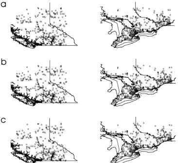
study regions (southern British Columbia/Alberta and southern Ontario/southwestern Québec) were chosen to represent a diverse range of topography and avail-able data. The BC/Alberta region extends across the Canadian Pacific coast, coastal and interior moun-tain ranges including the Rockies, and parts of the western boreal forest and prairies. As is typical in most parts of the world, climate data are particularly sparse in higher elevation areas. The Ontario/Québec region is comparatively flat but includes some higher elevation locations and areas downwind of the Great Lakes. In combination, these study areas represented the climatic conditions found in both forested and agricultural regions across much of southern Canada. The locations of the stations providing data for each variable in both regions are shown in Fig. 1. For each ofTmax,TminandP, respectively, data were available
from 434, 436 and 406 stations in the BC/Alberta region, and from 407, 405 and 371, stations in Ontario/Québec.
For each study region, approximately 50 stations were selected at random from the data set and with-held from the interpolation calculations. The perfor-mance of the two interpolation methods was then com-pared by using them both to estimate P, Tmax and
Tminat the coordinates of the withheld stations. Resid-uals were calculated as the differences between the estimated and observed values for each station for each month. Following Hulme et al. (1995) and Daly (1994), precipitation residuals were calculated as per-centage differences from the observed data. This ap-proach provides a better relative measure of the dif-ferences as compared to absolute values, particularly when the spatial variation in monthlyPis large, as is the case in BC. The residuals and squared residuals were pooled to determine Mean Errors (ME) and Root Mean Square Errors (RMSE), respectively.
Fig. 1. Locations of climate stations used for comparison of the GIDS and ANUSPLIN spatial interpolation methods, applied to 1961–1990 AES normals for study areas in British Columbia/Alberta (left) and Ontario/Qu´ebec (right). (a) monthly mean daily maximum temperature; (b) monthly mean daily minimum temperature; (c) monthly mean total precipitation. Symbols distinguish the stations used for interpolation (o) from those withheld as control stations used for error assessment (x).
a further assessment, the number of months in which one method gave lower RMSEs than the other were counted and checked for significance using a simple binomial test.
2.4. Map generation
To assess the behaviour of each interpolation method, maps were generated for a monthly vari-able giving poor agreement between observed and predicted data (July precipitation in the BC/Alberta study region was selected for this test). Using a 1 km Digital Elevation Model (DEM) for this region (ob-tained by resampling the GTOPO30 data set (Verdin
and Jenson, 1996) to a Lambert Conformal Conic projection), precipitation values were estimated for the centroids of each DEM pixel. The interpolated grids of precipitation data were then imported into ARC/INFO GRIDTMand printed as coloured images.
3. Results
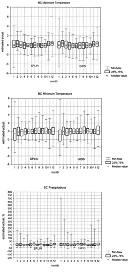
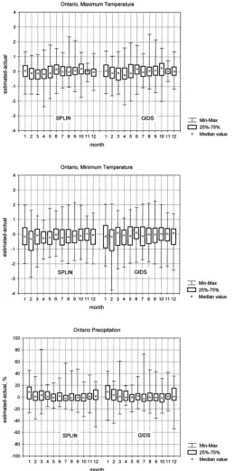
Figs. 2 and 3 present the box plots for BC/Alberta and Ontario/Québec respectively, for P, Tmax and
Tmin, obtained with ANUSPLIN and GIDS. Note
ally larger than those for Ontario/Québec. The box plots suggest that the two interpolation methods were generally comparable in their predictive accuracy, although careful inspection shows that ANUSPLIN performs rather better with the BC/Alberta data. In particular, the magnitudes of the residuals obtained for BC/Alberta precipitation are considerably larger using GIDS. The central tendency of the residuals resulted in generally small ME, confirming that both interpolators were substantially unbiased.
For temperature in Ontario/Québec, 50% of the predictions (the 25–75% percentiles) were generally within±0.5◦C of the recorded values. In most cases predictions fell within ±1◦C of the observed data,
although estimates of winter Tmin were noticeably
poorer. For most months, approximately half of the Ontario/Québec precipitation predictions were within
±10% of observed values, although the spread was generally wider for some winter months, particularly when using GIDS. Results for BC temperature were similar except that there were greater numbers of out-liers, and wider spreads for the 25–75% percentiles, with both interpolation methods. This is to be expected given the severe elevation gradients and the sparse coverage of climate stations sampling higher eleva-tion locaeleva-tions for extended periods. Both methods had greater difficulty predicting precipitation values in BC/Alberta for the withheld stations; i.e., several outliers exceeded 100% difference between observed and predicted data. The winter months of December, January and February were generally worst although GIDS had some greater residuals in April, October and November. Part of the explanation for this could be poorer quality data during winter months (e.g., difficulties in converting snowfall depth to equivalent water content), leading to greater variances in surface fitting and larger validation errors. Overall, the differ-ences in mean errors between the two interpolators were generally very small, but GIDS was more prone to extreme errors. This tendency is seen not only in the boxplots (Figs. 2 and 3), but was also reflected in the quality of the maps generated for the region (see Fig. 4).
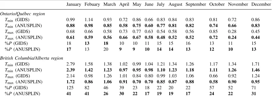
Table 1 compares pooled RMSE values obtained using the two interpolators for each of 72 cases (i.e., 12 months for three variables in two regions). Those obtained using ANUSPLIN were lower than those for GIDS in 70 out of the 72 possible cases. The
bino-mial test (assuming a null hypothesis of no difference between the two interpolation methods) showed this result to be highly significant for all three variables in both regions. For bothTminandTmax, ANUSPLIN
pro-duced lower mean RMSE in all 12 months (p≈0.0002) for both study regions. In the case ofP, mean RMSE was lower in all 12 months for BC/Alberta, but in only 10 months out of 12 (p<0.02) for Ontario/Québec.
Further inspection of Table 1 reveals that although the differences between the two interpolators were generally relatively small, the gains obtained from using ANUSPLIN were greatest in the most diffi-cult cases — i.e., BC/Alberta winter variables, where complex topography, low station density and poten-tially poorer quality measurements (mentioned ear-lier) were combined. In the particular case of winter precipitation in BC/Alberta (October–February inclu-sive), mean RMSE values obtained using GIDS were at least double those obtained from ANUSPLIN. Dif-ferences in mean RMSE for mid-winter temperature variables were also generally greater than for other months, although this effect is less pronounced for Ontario/Québec. Winter temperature data are more variable, for a number of possible reasons (e.g., for BC/Alberta, the standard deviations of the station ob-servations ofTmaxwere 5.5 and 2.8◦C for January and
July, respectively). With the exception of BC/Alberta winter precipitation, differences in RMSE between methods were always much smaller than the RMSEs obtained with either method.
Because GIDS is an exact interpolator, greater vari-ability results in a rougher surface, producing large RMSEs at locations between stations. In comparison, ANUSPLIN’s smoothing routines result in smaller av-erage errors in the interpolated surface. This tendency of ANUSPLIN to give lower RMSEs for temperature was supported by a visual comparison of maps gener-ated by the two interpolation methods for July mean
Tmaxin the BC/Alberta study region (data not shown). In this case, mean RMSEs were 0.85 and 0.99◦C for
Table 1
Summary of pooled Root Mean Square Error (RMSE) values obtained as the differences between observed and interpolated values for climate stations withheld from the analyses using GIDS and ANUSPLINa
January Febuary March April May June July August September October November December Ontario/Qu´ebec region
Tmin(GIDS) 0.99 1.14 0.93 0.72 0.86 0.66 0.83 0.84 0.83 0.81 0.72 0.86 Tmin(ANUSPLIN) 0.88 0.98 0.85 0.58 0.75 0.60 0.77 0.81 0.82 0.74 0.66 0.83
Tmax(GIDS) 0.68 0.66 0.58 0.73 0.77 0.63 0.54 0.58 0.56 0.85 0.28 0.45 Tmax(ANUSPLIN) 0.61 0.59 0.56 0.66 0.67 0.58 0.48 0.52 0.52 0.72 0.24 0.44
%P(GIDS) 18 13 18 10 10 11 15 15 16 13 11 15
%P(ANUSPLIN) 17 13 20 9 9 10 14 14 13 12 10 13
British Columbia/Alberta region
Tmin(GIDS) 2.79 1.58 1.38 1.02 0.99 1.04 1.21 1.34 1.26 1.17 1.34 1.71 Tmin(ANUSPLIN) 2.39 1.42 1.23 0.97 0.95 0.98 1.10 1.23 1.18 1.11 1.26 1.46
Tmax(GIDS) 2.14 0.98 1.26 1.01 0.84 0.80 0.99 1.03 1.06 0.66 0.92 1.24 Tmax(ANUSPLIN) 1.72 0.86 1.06 0.91 0.70 0.70 0.85 0.87 0.88 0.58 0.90 0.95
%P(GIDS) 125 82 46 39 23 18 22 20 22 57 52 71
%P(ANUSPLIN) 41 41 26 30 22 17 19 19 17 24 22 31
aIn total, 72 cases were compared — three variables for 12 months in two regions. Variables are monthly mean minimum and maximum temperatures in◦C (TminandTmax, respectively) and monthly mean total precipitation (P, with differences expressed as percentages). Bold face figures indicate the smaller RMSE obtained in each comparison.
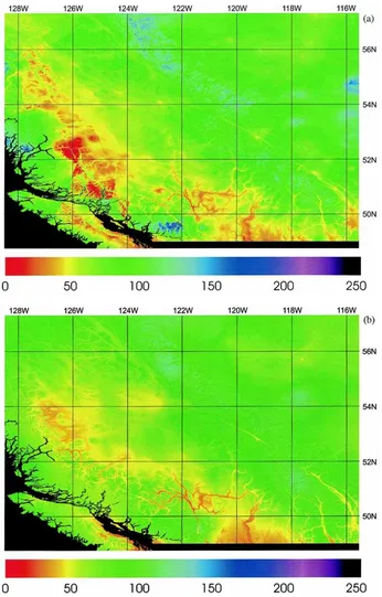
jected to a more inland climate despite its low eleva-tion. The small change in elevation relative to the coast generated an extremely large (inverted) lapse rate that GIDS applied to the higher elevation locations nearby. Figs. 2 and 3 show that the greatest differences be-tween interpolated values and observed data (in both means and variances) occurred for precipitation (as would be expected). The maps generated for July to-tal precipitation in BC/Alberta differ appreciably in visual terms (Fig. 4). As seen from Table 2, although the mean values differ only slightly, GIDS generates greater extremes of high and low precipitation, with a significantly larger standard deviation. The probable explanation for this is that GIDS is markedly more sensitive to local gradients derived from the station data (e.g., compare the Fraser Valley mountains at 49.5◦N 123.5◦W in Fig. 4a and b). In some cases,
these extremes are clearly unrealistic, particularly in
Table 2
Summary statistics for comparison of maps of July precipitation in British Columbia/Alberta study region (Fig. 4)a
GIDS ANUSPLIN
Minimum 0.0 15.0
Maximum 258.0 136.6
Mean 70.4 69.5
Standard deviation 23.3 17.8 aUnits are in mm.
the coastal mountain regions where zero precipita-tion is predicted for some summits (Fig. 4, 52.5◦N
126.0◦W). As with T
max on Vancouver Island, the
likely explanation is that large changes in precipitation with small changes in elevation close to sea level re-sult in significant underestimates when the gradient is applied at higher elevation. GIDS is clearly respond-ing to observations of extreme rainfall, e.g., at two lo-cations on the coast north of Vancouver Island, (Fig. 4, 52.5◦N 128.0◦W), where single stations evidently cause GIDS to estimate high rainfall in their immedi-ate vicinity. Conversely, the minimum curvature sur-faces fitted by ANUSPLIN minimise changes in gra-dients, giving rise to smoother transitions in surface values across the data network. These transitions are generally more interpretable and believable than those produced by GIDS. For example, Fig. 4 reveals some very abrupt boundaries between regions of high and low rainfall in the GIDS interpolation — particularly noticeable at the northern end of Vancouver Island (50.0◦N 126.5◦W) and on the mainland coast directly
opposite (51.0◦N 126.0◦W).
4. Discussion
methods, including kriging, in regions with sparse cov-erage of climate stations (Nalder and Wein, 1998), this study provided an important vindication of the advan-tages of using spline interpolation — at least for the range of climates occurring in Canada. Substantial ef-forts are currently being directed at producing high resolution digital climate grids using ANUSPLIN for Canada’s GIS, remote sensing and ecosystem mod-elling communities (McKenney et al., 1996). Never-theless, both interpolation methods performed reason-ably well in providing estimates of all variables in these two regions of the country.
The box plots revealed larger differences for the BC/Alberta region, particularly in the case of monthly mean precipitation. Paired t-tests performed on the RMSE values showed that the latter was the only sta-tistically significant case. This result is almost cer-tainly a consequence of the sparser station coverage and shorter records at high elevation sites in BC. In general, thin-plate smoothing splines such as ANUS-PLIN enable better prediction in such regions because they calibrate a spatially varying dependence on el-evation that uses all available data points. Although GIDS does respond to local gradients derived from the nearest data points, it can run into problems in moun-tainous regions where station coverage is sparse.
Perhaps the most serious problem with GIDS is that when the climate stations closest to the grid point are still a large distance away, the regression coefficients are relatively sensitive to the inclusion or exclusion of single stations. At these distances, even small changes in the coefficients can cause dramatic changes in the values predicted for the interpolation point. In those cases where the station being added to the set of closest stations contributes markedly different data to those from the station just removed (e.g., because one is at low elevation on the coast and the other is at higher elevation in a montane valley), abrupt boundaries will result. For example, the sharp boundary seen in Fig. 4a (around 51.0◦N 126◦W),
was caused by the station at Holberg, BC, (50.65◦N
128.0◦W, elevation 579 m, July precipitation 123 mm)
being replaced by a station at Campbell River, BC (50.05◦N 125.32◦W, elevation 31 m, July precipita-tion 46 mm). The large differences in elevaprecipita-tion and precipitation between these two stations caused a large change in the MLR coefficients, even though only one in 40 stations changed. The obvious
conclu-sion is that GIDS is not as appropriate for use in areas where climatic gradients are both steep and variable, e.g., for precipitation in mountainous regions.
When generating digital climate maps such as Fig. 4, it is difficult to say which of the two methods is more accurate, but the statistics for success in predicting the values at ‘withheld’ stations indicate that ANUSPLIN is superior. Subjective assessment of the maps shown in Fig. 4 confirms that the GIDS plot is ‘rougher’ — a consequence of it being an exact technique, i.e., the surface it generates passes through each climate station data value, which may result in unrealistically steep gradients at some locations. This is due mainly to the inverse-distance-squared averaging which causes the surface to form singularities around extreme values. It should be noted that some of these results might also be due to errors in the data — because large climate data sets are unlikely to be completely error-free! Both GIDS and ANUSPLIN have been used successfully to locate possible errors in source data. With ANUS-PLIN, stations with high residuals from the surface are sometimes found to be incorrectly geo-referenced or the datum has misplaced decimals. With GIDS, which does not smooth the data, errors have been revealed by checking for large differences between the interpolated values and observations withheld from the analysis.
shorter climate records that can reduce errors in inter-polated annual mean data by as much as 15%.
The results of our comparisons may be sensitive to edge effects. For these comparisons, climate stations outside each of the two defined regions were excluded, creating artificial edges. For a point near the edge of a region, predictions tend to be less accurate for two reasons: first, there are often fewer climate stations close to that point, and second, the climate stations do not surround the point which leads to a greater likeli-hood of extrapolation rather than interpolation. GIDS, in particular, is sensitive to edge effects because of its reliance on local gradients, e.g., for BC precipitation, pooled RMSE was 49% when only stations located within the defined BC/Alberta region were used for interpolation, but decreased to 26% when all available climate stations were used. It is clear that ANUSPLIN produces better results near the coast, where additional stations beyond the coast boundary are not available. Regardless, when using either interpolator to produce a definitive map, it will be desirable to include a gen-erous number of stations beyond the region of interest to minimize edge effects.
Both GIDS and ANUSPLIN have been shown to perform at least as well as universal kriging (Hutchin-son and Gessler, 1994; Nalder and Wein, 1998). One of the criticisms levelled at kriging is that it requires both questionable assumptions and some subjectivity in interpreting variograms prior to fitting the surface. Unlike GIDS, ANUSPLIN does require an ele-ment of subjectivity when fitting surfaces for large geographic regions. In such cases (specifically not including the study reported here),‘knots’ (i.e., repre-sentative climate stations) are required. The subjec-tivity comes in deciding how many knot stations to use to obtain an optimal fit of the spline surface to the data and the most appropriate level of data smooth-ing. Once this number has been set, knot stations are selected automatically by ANUSPLIN’s ‘Selnot’ pro-cedure, after which, interpolation proceeds relatively quickly. The GCV statistic generated by ANUSPLIN assists in objectively identifying the ‘best’ surface, and hence in determining which stations to include as knots. The GCV can be interpreted as a spatially av-eraged standard error, where the calculated standard errors approximate the GCV over the region covered by the data network, but increase outside the region (see Hutchinson and Gessler, 1994). In the present
study, the RMSE values for the withheld data were all similar to the root GCVs — hence providing a useful independent validation of the GCV statistic. In com-parison, GIDS is a ‘brute-force’ method that requires no optimization — which may be a problem when using it to generate large grids. While ANUSPLIN can in principle be used to generate grids over large areas relatively quickly from a single fitted surface, the potentially limited number of knots may result in lower accuracy — although preliminary tests on Cana-dian data suggest this effect is not significant (D.W. McKenney, personal communication, 1999). If a se-rious reduction in accuracy does occur, the remedy is to break the area of interest into multiple overlapping patches where each patch has its own set of spline co-efficients, derived from all the available stations. This could result in discontinuities at the boundaries of the overlapping patches when creating composite maps, but again, this has not been found to be a significant problem.
The results from both methods could likely be re-fined in actual applications e.g., by adding distance from large water bodies or slope aspect as indepen-dent variables. This capacity is already present within GIDS and ANUSPLIN — the challenge is developing the required data for both the interpolation component and the grids. The number of independent variables used by GIDS would be limited only by the avail-ability of data. A new national DEM created by the Canadian Forest Service and the Canada Centre for Topographic Information (D.W. McKenney, personal communication, 1999), will enable some of these research issues to be investigated further.
re-sults for interpolating long climate histories over ex-tensive regions. The results of the present study sug-gest that ANUSPLIN should produce better monthly products, but other techniques, including GIDS, could still prove useful.
One example of an alternative interpolator is the PRISM model developed by Daly (Daly, 1994; Daly et al., 1997; Daly and Johnson, 1999), which is being used to prepare monthly precipitation and tempera-ture maps for southern British Columbia (Eric Taylor, Canadian Atmospheric Environment Service, personal communication, 1999). PRISM is a knowledge-based approach that combines local regression-based map output with interpretation and evaluation by human experts. The knowledge base supporting PRISM fea-tures several station-weighting functions, including: multi-scale topographic facets to simulate rain shad-ows; a two-layer atmosphere to account for temper-ature inversions and mid-slope precipitation maxima; coastal proximity to handle climate gradients along coastal strips; and effective terrain height to account for the varying effects of topographic barriers on pre-cipitation. These ‘expert’ weighting functions simulate identifiable climatological processes that have been in-vestigated and validated in regions where such data are available, and are then assumed to apply to broadly comparable regions where data are scarce (Christo-pher Daly, Oregon State University, personal commu-nication, 1999). Such an approach may be useful in mountainous regions where high elevation locations are often under-represented by long-term observing stations. These assumptions should be tested for each application, however, because it is possible that the expert weightings will instead lead to increased biases in the interpolated values. Unfortunately, testing can be problematic since the greatest bias will generally occur in the locations where validation data are par-ticularly sparse.
5. Conclusions
In a comparison of two elevation-dependent spa-tial interpolators applied to 30-year monthly climate means for selected regions of Canada, the ANUSPLIN method developed by Hutchinson (1995a) proved gen-erally superior to the GIDS method of Nalder and Wein (1998). Both subjective assessment and
statis-tical analyses showed that ANUSPLIN is generally more accurate in predicting climate variables at the locations of climate stations withheld at random from the source datasets. Additionally, ANUSPLIN is able to generate smoother and more credible gradients at regional boundaries and at locations where climate sta-tion coverage is poor, notably at higher elevasta-tion sites. The generally better accuracy of a thin plate spline oc-curs because it better calibrates a continuous spatially varying dependence on elevation using all available data points. This explains why local regression meth-ods (such as GIDS) can have difficulties in areas with non-uniform gradients.
GIDS is a useful technique nevertheless, because it is relatively intuitive, objective and easy to imple-ment, and performs well in comparison to most other commonly used spatial interpolation methods. It thus provides a useful standard against which to compare more sophisticated interpolators such as ANUSPLIN. Both methods have the potential for increased accu-racy by introduction of additional independent vari-ables known to have effects on local climate.
Acknowledgements
Kathy Campbell, Kevin Lawrence, Pia Papadopol and Marty Siltanen of Canadian Forest Service pro-vided technical support in statistical analysis and in generation of the figures. We would also like to thank Bill Hogg and Anna Deptuch-Stapf of Environment Canada for provision of data and encouragement in creating gridded climatologies for Canada.
References
Boer, G.J., McFarlane, N.A., Lazare, M., 1992. Greenhouse gas-induced climate change simulated with the CCC second-generation general circulation model. J. Climate 5, 1045–1077.
Caya, D., Laprise, R., Giguère, M., Bergeron, G., Blanchet, J.P., Stocks, B.J., Boer, G.J., McFarlane, N.A., 1995. Description of the Canadian regional climate model. Water Air Soil Pollut. 82, 477–482.
Daly, C., 1994. A statistical-topographic model for mapping climatological precipitation over mountainous terrain. J. Appl. Meteorol. 33, 140–158.
Climatology, 79th Annu. Meeting Am. Meteorol. Soc., Dallas, TX, 49 pp.
Daly, C., Taylor, G.H., Gibson, W.P., 1997. The PRISM approach to mapping precipitation and temperature. Proc. 10th Conf. on Applied Climatology, Reno, NV. Am. Meteorol. Soc., pp. 10–12.
Environment Canada, 1994. Canadian Monthly Climate Data and 1961–1990 Normals on CD-ROM Version 3.0E.
Houghton, J.T., Meira Filho, L.G., Callander, B.A., Harris, N., Kattenberg, A., Maskell, K. (Eds.), 1996. Climate Change 1995: the science of climate change. Cambridge University Press, Cambridge.
Hughes, D.A., 1982. The relationship between mean annual rainfall and physiographic variables applied to a coastal region of southern Africa. S. African Geographic J. 64, 41–50. Hulme, M., Conway, D., Jones, P.D., Jiang, T., Barrow,
E.M., Turney, C., 1995. Construction of a 1961–1990 European climatology for climate change modelling and impact applications. Int. J. Climate 15, 1333–1363.
Hutchinson, M.F., 1984. Some surface fitting and contouring programs for noisy data. CSIRO Division of Mathematics and Statistics, Consulting Report ACT 84/6, Canberra.
Hutchinson, M.F., 1991. The application of thin-plate smoothing splines to continent-wide data assimilation. In: Jasper, J.D. (Ed.), Data assimilation systems. BMRC Res. Report No. 27, Bureau of Meteorology, Melbourne, pp. 104–113.
Hutchinson, M.F., 1995a. Interpolating mean rainfall using thin plate smoothing splines. Int. J. GIS 9, 385–403.
Hutchinson, M.F., 1995b. Stochastic space-time weather models from ground-based data. Agric. For. Meteorol. 73, 237–264. Hutchinson, M.F., 1998a. Interpolation of rainfall data with thin
plate smoothing splines I. Two dimensional smoothing of data with short range correlation. J. Geographic Information Decision Analysis 2, 153–167.
Hutchinson, M.F., 1998b. Interpolation of rainfall data with thin plate smoothing splines II. Analysis of topographic dependence. J. Geographic Information Decision Analysis 2, 168–185. Hutchinson, M.F., 1999. ANUSPLIN Version 4.0. http://
cres.anu.edu.au/software/anusplin.html
Hutchinson, M.F., Bischof, R.J., 1983. A new method of estimating mean seasonal and annual rainfall for the Hunter Valley, New South Wales. Aust. Meteorol. Mag. 31, 179–184.
Hutchinson, M.F., Gessler, P.E., 1994. Splines — more than just a smooth interpolator. Geoderma 62, 45–67.
Jones, P.G., Thornton, P.E., 1997. Spatial and temporal variability of rainfall related to third order Markov model. Agric. For. Meteorol. 86, 127–138.
Mackey, B.G., McKenney, D.W., Yang, Y.Q., McMahon, J.P., Hutchinson, M.F., 1996. Site regions revisited: a climatic analysis of Hill’s site regions for the province of Ontario using a parametric method. Can. J. For. Res. 26, 333–354. McKenney, D.W., Mackey, B.G., Sims, R.A., 1996. Primary
databases for forest ecosystem management — examples from Ontario and possibilities for Canada: NatGRID. Environmental Monitoring Assessment 39, 399–415.
McKenney, D.W., Kesteven, J.L., Hutchinson, M.F., Venier, L., 2000. Canada’s plant hardiness zones revisited, submitted for publication.
Nalder, I.A., Wein, R.W., 1998. Spatial interpolation of climatic Normals: test of a new method in the Canadian boreal forest. Agric. For. Meteorol. 9, 211–225.
Nalder, I.A., Wein, R.W., 2000. Long-term forest floor carbon dynamics after fire in upland boreal forests of western Canada. Global Biogeochem. Cycles, in press.
Nalder, I.A., Price, D.T., Wein, R.W., 2000. Can patch models replicate observed stand dynamics? A test of BORFOR and FORSKA2V in the boreal forests of western Canada. Ecol. Modelling, submitted for publication.
Phillips, D.L., Dolph, J., Marks, D., 1992. A comparison of geostatistical procedures for spatial analysis of precipitation in mountainous terrain. Agric. For. Meteorol. 58, 119– 141.
Press, W.H., Flannery, B.P., Teukolsky, S.A., Vetterling, W.T., 1986. Numerical Recipes. Cambridge University Press, Cambridge, 818 pp.
Price, D.T., Nalder, I.A., Siltanen, R.M., 1998. A 10-km national climate surface for Canadian global change studies. In: Marceau, D. (Ed.), Scaling and modelling in forestry: applications in remote sensing and GIS. Université de Montréal, Montréal, pp. 161–168.
Racsko, P., Szeidl, L., Semenov, M., 1991. A serial approach to local stochastic weather models. Ecol. Modelling 57, 27–41. Richardson, C.W., 1981. Stochastic simulation of daily
precipitation, temperature and solar radiation. Water Resources Res. 17, 182–190.
Snyder, J.P., 1987. Map Projections — A Working Manual. U.S. Geological Survey Professional Paper 1395. U.S. Govt. Print. Off., Washington DC, 383 pp.+poster.
Shepard, D.L., 1968. A two dimensional interpolation function for irregularly spaced data. Proc. 23rd Nat. Conf., Assoc. Computing Machinery, ACM, Washington, pp. 517–524. Thiessen, A.H., 1911. Precipitation averages for large areas.
Monthly Weather Rev. 39, 1082–1084.
Venier, L.A., McKenney, D.W., Wang, Y., McKee, J., 1998a. Models of large-scale breeding-bird distribution as a function of macroclimate in Ontario, Canada. J. Biogeography 26, 315– 328.
Venier, L.A., Hopkin, A.A., McKenney, D.W., Wang, Y., 1998b. A spatial climate-determined risk rating for Scleroderris disease of pines in Ontario. Can. J. For. Res. 28, 1398– 1404.
Verdin, K.L., Jenson, S.K., 1996. Development of continental scale DEMs and extraction of hydrographic features. Integrating GIS and Environmental Modeling, Sante Fe, New Mexico: National Center for Geographic Information and Analysis (NCGIA). See also: http://edcwww.cr.usgs.gov/ webglis/glisbin/guide.pl/glis/hyper/guide/gtopo 30
Wahba, G., 1990. Spline models for observational data. CBMS-NSF Regional Conf. Ser. Appl. Math., Philadalphia Soc. Ind. Appl. Math., 169 pp.
Wahba, G., Wendelberger, J., 1980. Some new mathematical models for variational objective analysis using splines and cross validation. Monthly Weather Rev. 108, 1122–1143.