MODEL-CHECKS FOR HOMOSCHEDASTIC SPATIAL LINEAR REGRESSION MODEL BASED ON BOOTSTRAP METHOD | Somayasa | JURNAL ILMIAH MATEMATIKA DAN TERAPAN 138 470 1 PB

W. Somayasa

Mathematics Department of Haluoleo University, Kendari email: wayan.somayasa@yahoo.de

Abstract

In this paper we propose Efron residual based-bootstrap approximation methods in asymptotic model-checks for homoschedastic spatial linear regression models. It is shown that under some regularity conditions given to the known regression functions the bootstrap version of the sequence of least squares residual partial sums processes converges in distribution to a centred Gaussian process having sample paths in the space of continuous functions on

I

:

0

,

1

0

,

1

. Thus, Efron residual based-bootstrap is a consistent approximation in the usual sense. The finite sample performance of the bootstrap level Kolmogorov-Smirnov (KS) type test is also investigated by means of Monte Carlo simulation.

Key words: residual based-bootstrap, asymptotic model-check, homoschedastic spatial linear regression models, partial sums, Gaussian process.

I. Introduction

Practically the correctness of the assumed linear models is usually evaluated by analysing the

cumulative sums (CUSUM) of the least squares residuals. To this end a huge amount of literature is available, see among others MacNeill (1978) or Bischoff and Miller (2000) for one dimensional

context. In the spatial context we refer the reader to MacNeill and Jandhyala (1993) and Xie and MacNeill (2006).

To see the above mentioned problem in more detail let us consider an experiment performed

on an experimental region

I

:

0

,

1

0

,

1

under

n

2 experimental conditions taken from a regular lattice, given by

I

n

k

,

1

:

)

n

/

k

,

n

/

(

:

n





,

n

1

. (1)

Accordingly, we put together the observations carried out in _n in an

n

n

matrix n

n n

, n

1 , 1 k k n

n

:

Y

Y

_{ } , where for

1



,

k

n

,

Y

_k is the observation at the point

)

n

/

k

,

n

/

(



, and n n is the space of

n

n

real matrices furnished with the Euclidean inner

product

A

,

B

n n

:

trace

(

A

t

B

)

and the corresponding norm given by

)

A

A

(

trace

A

n n t , for

A

,

B

n n. It is worth noting that for our model we take

I

as the

experimental region without loss of generality instead of any compact subset of 2. For any

I

:

f

, let

f

(

_n

)

:

f

(



/

n

,

k

/

n

)

_kn,n_{1, 1} n n, then we have

Y

_{n n}

g

(

_n

)

E

_{n n},

Model-Checks For Homoschedastic Spatial Linear Regression Model Based On Bootstrap Method

n , n

1 , 1 k k n

n

:

E

_{ } is the corresponding matrix of independent and identically distributed random

errors having mean zero and variance 2

(

0

,

)

, for

1



,

k

n

. We are interested in testing

the hypotheses

n n 0

:

g

(

)

W

H

vs.

K

:

g

(

_n

)

W

_n,

n

1

, (2)

where

W

_n

:

f

₁

(

_n

),



,

f

_p

(

_n

)

n n is a sub space of n n generated by

f

₁

(

_n

)

,



,

)

(

f

_{p n} .

Under

H

₀, the matrix of least squares residuals is given by

n n n W n n n W n

n

:

pr

Y

pr

E

R

(Stapleton, 1995), where

n W

pr

is the orthogonal projector onto

the orthogonal complement of

W

_n. Without loss of the generality we assume throughout this work

that

f

₁

(

_n

)

,



,

f

_p

(

_n

)

is an orthogonal basis of

W

_n. Hence, by the elementary linear algebra we get under

H

₀,

p

1

i _{i n i n}

n i n

n n i n

n n n

n n n n

)

(

f

),

(

f

)

(

f

E

),

(

f

E

:

R

. (3)

Equivalently by the

vec

operator, we have

vec

(

R

_{n n}

)

vec

(

E

_{n n}

)

X

_n

(

X

t_n

X

_n

)

1

X

t_n

vec

(

E

_{n n}

)

,

where

X

_n is the design matrix of the model under

H

₀, i.e., an

n

2

p

matrix whose

k

th column

is given by the

n

2 dimensional vector

vec

(

f

_k

(

_n

))

,

k

1

,



,

p

. A consistent estimator for 2

is given by

p

n

R

:

ˆ

₂

2 n n 2 n

n n

in the sense

ˆ

_n2 converges in probability to 2, as

n

.

Suppose that the regression functions

f

₁,



,

f

_p are linearly independent and squared integrable on I with respect to the Lebesgue measure _I, then under

H

₀, MacNeill and Jandhyala

(1993) and Xie and MacNeill (2006) showed that

)

(

B

)

))(

R

(

vec

(

T

_{n n n} D _f

n

1 _in

C

I

_{, as}

n

_,

where for

(

t

,

s

)

I

,

) R (

I 2 1

s , 0 t , 0

I t 2

f

(

t

,

s

)

:

B

(

t

,

s

)

f

d

G

fdB

B

, (4)

and

T

_n

:

n2

C

(

I

)

is the partial sums operator defined in Park (1971). Here

p p p

, p

1 , 1 k I I

k

f

d

f

:

G



 ,

B

2 is the standard Brownian sheet having sample pats in

C

I

and ) R (

If

t

_n is a realisation of the Kolmogorov-Smirnov (KS) statistics

)

n

/

k

,

n

/

))(

R

(

vec

(

T

n

1

max

:

KS

_{n n n}

n k , 0 f ,

n _



, then a level test of KS type based on residual

partial sums processes for testing (2) will reject

H

₀ if and only if

t

_n

c

₁ , where

c

₁ is a constant that satisfies the equation

_{n n n 1}

n k , 0 0

H

T

(

vec

(

R

))(

/

n

,

k

/

n

)

c

n

1

max

P



 .

Hence, by the continuous mapping theorem (Billingsley, 1968, p. 29-30),

c

₁ can be approximated by means of the distribution of

sup

B

f

(

t

,

s

)

1 s , t 0

.

As it is presented in (4), the limiting distribution of the KS type statistics under

H

₀ is not

mathematically tractable, because it depends on the structure of the designs and the regression functions. Therefore the application of the preceding tests procedure is limited. It is the purpose of

the preceding paper to investigate the performance of bootstrap test of (2). Although the application of the bootstrap appears naturally in the present context, to the knowledge of the author this topic

has not found much attention in the literature. One purpose of the present paper is to demonstrate that Efron residual based-bootstrap (Shao and Tu, 1995) provides simple and reliable alternative for

constructing asymptotic critical region of such a KS type test. This will be discussed in the Section 2. In Section 3 we develop Monte Carlo simulation in investigating the finite sample characteristics of

the bootstrap test. An application of the developed method to a real data will be presented in Section 4. Finally we close the paper in Section 5 presenting conclusion and some remarks for future

researches.

II. Bootstrap Approximation

Let

r

_kbe the component of the residual matrix in the

k

th row and



thcolumn computed based on the original observations

Y

_{n n} under

H

₀,

1



,

k

n

. We define an

n

n

matrix of

centred residuals

R

ˆ

_{n n}

:

r

_k

r

_kn,n_{1, 1}, where

n

1 k n

1 k 2 n

1

r

:

r

 

. Further, let Rˆ

F

be the

empirical distribution function of the components of

R

ˆ

_{n n} putting mass ₂ n

1 _to

r

r

k

 , for

n

k

,

1



, i.e., for

x

, n

1 k

n

1 ,x k

2 n

1

Rˆ

(

x

)

:

1

(

r

r

)

F

 

, where

1

_A is the indicator function

of

A

. Efron residual based-bootstrap defines the bootstrap observations by

* n n n n

, n

1 , 1 k *

k *

n

n

:

Y

g

(

)

E

Y

 _ ,

where

E

*_{n n}

:

*_k n_k,n_1,1 is a random matrix whose components are a random sample from

F

_Rˆ

and

)

(

g

_n p

1

i _{i n i n n n}

n i n n n n n i

)

(

f

),

(

f

)

(

f

Y

),

(

f

Model-Checks For Homoschedastic Spatial Linear Regression Model Based On Bootstrap Method

is the ordinary least squares estimator of

g

(

_n

)

under

H

₀. Let

E

* and

var

* be the expectation and variance operators conditioned on

Rˆ

F

. Then by the construction it is clear that

E

*

(

_*_k

)

0

and _{2 n}2 2

n p 2 n * k * 2 *

n

:

var

(

)

ˆ

(

r

)

ˆ

 which clearly converges in probability to

2

by the

famous weak law of large number and Slutsky’s theorem.

The bootstrap analogous of the residual partial sums process is given by

T

(

vec

(

R

))(

)

ˆ

n

1

* n n n * n

)

))(

E

(

vec

X

)

X

X

(

X

)

E

(

vec

(

T

ˆ

n

1

* n n t n 1 n t n n * n n n * n

. (6)

Hence, the bootstrap version of the KS type statistics can be represented by

T

(

vec

(

R

))(

/

n

,

k

/

n

)

ˆ

n

1

max

:

KS

* n *n n

n n k , 0 * f , n



 . (7)

Theorem 1

Suppose that the regression functions

f

₁,



,

f

_p are linearly independent in the space of squared integrable functions with respect to _I, denoted by

L

₂

(

_I

)

, continuous and have bounded variation on I. Then under

H

₀ it holds,

T

(

vec

(

R

))(

)

ˆ

n

1

_* n n n * n

)

(

B

_f D

in

C

I

, as

n

.

Proof

For any rectangle

A

:

t

1

,

t

2

s

1

,

s

2

I

,

2

t

1

t

,

s

1

s

2

and any real-valued function

f

on

I

, the increment of

f

over A is defined by

)

2

s

,

2

t

(

f

:

f

I

-

f

(

t

2

,

s

1

)

f

(

t

1

,

s

2

)

f

(

t

1

,

s

1

)

.

Further, for a fixed natural number n, let us define operators

U

_n

:

C

(

I

)

n2 and

)

I

(

C

)

I

(

C

:

O

_n , such that for any

u

C

(

I

)

and

(

t

,

s

)

I

, n , n 1 , 1 k k I n

(

u

)

:

vec

u

U



 , (8)

)

s

,

t

(

)

u

(

U

X

)

X

X

(

X

)

u

(

U

T

:

)

s

,

t

)(

u

(

O

_{n n n n} t_{n n} 1 t_{n n} , (9)

where

I

_k

:

(



1

)

/

n

,



/

n

(

k

1

)

/

n

,

k

/

n

,

1



,

k

n

. It is obvious that

O

_n is linear by

the linearity of

T

_n. Moreover, since for every

a

n2,

U

_n

(

T

_n

(

a

))

a

, it follows that

O

_n is idempotent. It can also be shown by the expression

)

s

,

t

))(

u

(

U

(

T

)

s

,

t

)(

u

(

O

_{n n n}

p

1

i _{i n i n}

n i n n n i

))

(

f

(

vec

)),

(

f

(

vec

)

s

,

t

)))(

(

f

(

vec

(

T

)

u

(

U

)),

(

f

(

vec

,

by the definition of norm of a operator on Banach space (Conway, 1985, p. 70), that

p 1 i 2 i 1 s , t 0 2 i

n

13

1

4

f

inf

f

(

t

,

s

)

Thus,

O

_n is uniformly bounded on

C

(

I

)

. This will directly imply to the continuity of

O

_non

C

(

I

)

,

where

.

is the supremum norm. Let us define an operator

O

:

C

(

I

)

C

(

I

)

, such that for every

)

I

(

C

u

and

(

t

,

s

)

I

,

) R (

I 1

s , 0 t , 0

I t s

, 0 t ,

0

u

f

d

G

fdu

:

)

s

,

t

)(

u

(

O

.

The right hand side of (9) also can be written by

)

s

,

t

(

)

u

(

U

T

:

)

s

,

t

)(

u

(

O

_{n n n}

)

u

(

U

X

X

X

n

1

X

n

1

n t n n t n 2 n t

ns nt

2 ,

where _{nt ns} n2is the vector whose first

nt

ns

components are one and the reminder is zero. By the definition and by the continuity of

u

, we have

T

U

(

u

)

(

t

,

s

)

0,t 0,s

u

n n

n ,

(

t

,

s

)

I

. (10)

Furthermore, since for

i

1

,



,

p

,

f

_i is bounded on I, then it holds component wise

n t

ns nt

2

X

n

1

s , 0 t 0,

I p s

, 0 t , 0

I 1 n

d

f

,

,

d

f



. (11)

The convergence component wise

1

n t n 2

X

X

n

1

1

1 p , p

1 j , 1 i I

I j i n

G

d

f

f

, (12)

follows from the fact that the mapping

B

B

1 is continuous on the space of invertible matrices. Further, since for

i

1

,



,

p

,

f

_i has bounded variation and

u

is continuous on I, the Riemann-Stieltjes integral of

f

_i with respect to u exists for all i. Consequently, we have the following convergence component wise

)

u

(

U

X

t_{n n}

) R (

I p )

R (

I 1 n

du

f

,

,

du

f



. (13)

Thus, from (10), (11), (12) and (13) , for every

u

C

(

I

)

, it holds

O

_n

(

u

)

O

(

u

)

n

0

.

Next let

(

u

_n

)

_{n 1} be any sequence in

C

(

I

)

such that

u

_n

u

n

0

, then since

O

_nis bounded on

C

(

I

)

, we finally have

)

u

(

O

)

u

(

O

0

n n

O

_n

u

_n

u

O

_n

(

u

)

O

(

u

)

n

0

.

The last result shows that the only subset of

C

(

I

)

that satisfies the condition there exists a

sequence

(

u

_n

)

_{n 1} that converges to u in

C

(

I

)

, but the sequence

(

O

_n

(

u

_n

))

_{n 1} does not converge to

O

(

u

)

is an empty set. Hence, by Theorem 5.5 in Billingsley (1968) and Theorem 4 in Park

Model-Checks For Homoschedastic Spatial Linear Regression Model Based On Bootstrap Method

T

vec

(

E

)

ˆ

n

1

O

)

R

(

vec

T

ˆ

n

1

*

n n n

* n n *

n n n

* n

)

B

(

O

₂

D

, as

n

.

The proof of the theorem is complete since

B

2

(

t

,

s

)

0

, almost surely if

t

0

or

s

0

. Corollary 1

By the continuous mapping theorem, under

H

₀ we have

KS

Sup

B

_f

(

t

,

s

)

1 s , t 0 D *

f ,

n , as

n

.

Hence, for

(

0

,

1

)

, the constant

c

₁ defined in page 4 can now be approximated by the

constant

c

₁* that satisfies the equation

P

*

KS

*_n,f

c

₁* . If

t

_n is a realisation of

KS

_n,f,

then an asymptotic level KS type test will reject

H

₀ if

t

_n

c

₁* . We will illustrate in Section 4 the finite sample properties of this approach by means of simulation study.

Remark 3.

The extension of Theorem 1 to the case of

p

3

dimensional unit cube and experimental

design

n

₁

n

₂



n

_p regular lattice with

n

_i

n

_j, for

i

j

is straightforward.

III. Simulation

We develop Monte Carlo simulation for constructing the finite sample sizes critical region of

the bootstrap level test of the hypotheses

W

g

:

H

₀ vs.

K

:

g

W

'

, (15)

where

W

:

f

₁

,

f

₂

,

f

₃ and

W

'

:

f

₁

,

f

₂

,

f

₃

,

f

₄

,

f

₅

,

f

₆ ,

f

₁

,

f

₂,

f

₃,

f

₄,

f

₅,

f

₆

:

I

, defined by

f

₁

(

t

,

s

)

:

1

,

f

₂

(

t

,

s

)

:

t

,

f

₃

(

t

,

s

)

:

s

,

f

₄

(

t

,

s

)

:

t

2,

f

₅

(

t

,

s

)

:

ts

, and

f

₆

(

t

,

s

)

:

s

2. The simulation is developed according to the following algorithm.

Begin Algorithm

Step 1: Generate

n

n

matrix of pseudo random errors

E

_{n n}from a distribution having mean zero and variance 2.

Step 2: Compute the least squares residuals by the equation

)

E

(

vec

X

)

X

X

(

X

)

E

(

vec

)

R

(

vec

_{n n n n n} t_{n n} 1 t_{n n n} .

Step 3: Generate

n

n

matrix of bootstrap errors

E

*_{n n}by sampling with replacement from the

centred residuals.

Step 4: Compute the bootstrap residuals by the equation

)

E

(

vec

X

)

X

X

(

X

)

E

(

vec

)

R

(

vec

*_{n n n}* _{n n n}t _n 1 _nt *_{n n} .

Step 5: Compute

ˆ

*_n and

KS

*_n,f.

Step 6: Repeat Step 1 to Step 5 M times.

Step 7: Compute

c

*₁ : sort M values of

KS

*_n,fobtained in Step 5 in ascending order, i.e., )

2 *(

f , n ) 1 *(

f ,

n

KS

KS



*(M)

f , n

then

Ν

α)

-(1

M

if

;

KS

Ν

α)

-(1

M

if

;

KS

c

1) α) (1 *(M

f n,

α)) (1 *(M

f n, *

1 ,

where

N

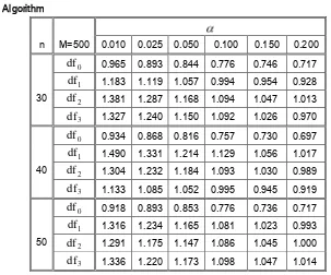
is the set of natural numbers. End Algorithm

n M=500 0.010 0.025 0.050 0.100 0.150 0.200

30 0

df

0.965 0.893 0.844 0.776 0.746 0.717

1

df

1.183 1.119 1.057 0.994 0.954 0.928

2

df

1.381 1.287 1.168 1.094 1.047 1.013

3

df

1.327 1.240 1.150 1.092 1.026 0.970

40 0

df

0.934 0.868 0.816 0.757 0.730 0.697

1

df

1.490 1.331 1.214 1.129 1.056 1.017

2

df

1.304 1.232 1.184 1.093 1.030 0.989

3

df

1.133 1.085 1.052 0.995 0.945 0.919

50 0

df

0.918 0.893 0.853 0.776 0.736 0.717

1

df

1.316 1.234 1.165 1.081 1.023 0.993

2

df

1.291 1.175 1.147 1.086 1.045 1.000

3

[image:7.516.73.376.155.407.2]

df

1.336 1.220 1.173 1.098 1.047 1.014 Table 1. Simulated rejection probabilities of the Kolmogorov-Smirnov bootstrap test.

For the simulation, we generate the error variables from i.i.d. random variables having mean zero and variance 0.5. Four cases are considered, that is for

1



,

k

n

,

_k

~

N

(

0

,

0

.

5

)

and _k

~

2

4

,

1

,

2

,

3

.

The simulation results are depicted in Table 1 for the sample sizes

n

30

,

40,

50

and 60 and level 1%, 2.5%, 5%,

10

%

, 15%, and 20% with 500 replications. The entries in the row named

df

₀ are simulation results for which the errors are generated from

N

(

0

,

0

.

5

)

, whereas those in the

rows named

df

are generated from chi-square distribution having

1

,

2

,

3

degrees of freedom such that

E

(

_k

)

0

and

var(

_k

)

0

.

5

, for

1



,

k

n

. We note that for the simulation the generation of the random errors are restricted neither to a specific family of distributions nor to the distribution having variance 0.5 only. The variance as well as the family of the distribution may vary

as long as they satisfy the conditions specified in Theorem 1. IV. Example

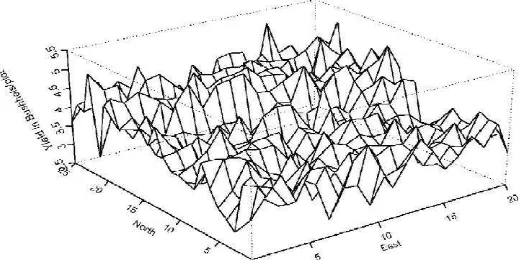
As an example we consider the wheat-yield data (Mercer and Hall’s data) presented in Cressie (1993), p. 454-455. The data are yield of grain (in pounds) observed over a 25 x 20 lattice of

Model-Checks For Homoschedastic Spatial Linear Regression Model Based On Bootstrap Method

The experiment consists of giving the 500 plots the same treatment (presumably fertilizer, water,

etc.), from which it can be identified that the data are a realization of 500 independent random variables. As was informed in Cressie (1993), the plots are assumed to be equally spaced with the

dimension of each plot being 10.82 ft by 8.05 ft. Figure 2 presents the perspective plot of the data. Observing Figure 2, we postulate under

H

₀ a first order polynomial model as in Hypothesis

(16). Since the variance is unknown, we use a consistent estimator

ˆ

_nm2 . Calculated under

H

₀, the

data give

ˆ

_nm2 = 0.1898, where

3

nm

)

(

f

),

(

f

)

(

f

Y

),

(

f

Y

ˆ

2

m n 3

1

i _{i nm i nm n m}

nm i m n m n nm i m n

2

nm ,

20

k

1

,

25

1

:

)

20

/

k

,

25

/

(

nm





. The functions

f

1

,

f

2, and

f

3 are defined as in Section 4. After computation, we get the critical value of the KS type test 1.5919, so bootstrap approximation of the p-value of the test computed by simulation is given by

ˆ

= 0.0001. Thus it can [image:8.516.127.387.322.453.2]

be concluded that

H

₀ is rejected for all suitable values of .

Figure 2. The perspective plot of Mercer and Hall’s data

V. Concluding Remark

Efron residual based-bootstrap approximation to the KS type statistics based on least squares residual partial sums processes of homoschedastic spatial linear regression model is consistent. In

the forthcoming paper we shall investigate the application of Efron as well as wild bootstrap in the case of heteroschedastic spatial linear regression model.

The experimental design considered so far is restricted to the regular lattice on the unit square I, since the prerequisite condition of the theory is satisfied well. In practice this situation is

sometimes not reasonable, therefore we need to develop the theory in more general setting. VI. References

2. Bischoff, W. and Miller, F., 2000, Asymptotically Optimal Tests and Optimal Designs for Testing the Mean in Regression Models with Application to Change-Point Problems, Ann.

Inst. Statist. Math. Vol. 52, 658-679.

3. Conway, J.B., 1985, A Course in Functional Analysis, Springer-Verlag New York Inc., New York.

4. Cressie, Noel A. C., 1993, Statistics for Spatial Data, Revised Edition, John Wiley & Sons, Inc, New York, Singapore, Toronto.

5. MacNeill, I.B., 1978, Properties of Sequences of Partial Sums of Polynomial Regression Residuals with Applications to Tests for Change of Regression at Unknown Times,

Ann. Statist. Vol. 6, 422-433.

6. MacNeill, I.B. and Jandhyala, V.K., 1993, Change Point Methods for Spatial Data, Multivariate Environmental Statistics, eds. by G.P. Patil and C.R. Rao, Elsevier Science

Publishers B.V., 298-306.

7. Park, W.J., 1971, Weak Convergence of Probability Measures on the Function Space

)

1

,

0

(

C

2 _{, J. of Multivariate Analysis. Vol. 1, 433-444.}

8. Shao, J. and Tu, D., 1995, The Jackknife and Bootstrap, Springer-Verlag, New York.

9. Stapleton, J. H., 1995, Linear Statistical Model, John Wiley & Sons Inc, New York, Toronto,

Singapore.

10. Xie, L. and MacNeill, I.B., 2006, Spatial Residual Processes and Boundary Detection, South