Semi-supervised learning
Alejandro Cholaquidisa, Ricardo Fraimana and Mariela Suedb a CABIDA and Centro de Matem´atica,
Facultad de Ciencias, Universidad de la Rep´ublica, Uruguay b Instituto de C´alculo,
Facultad de Ciencias Exactas y Naturales, Universidad de Buenos Aires
Abstract
Semi-supervised learning deals with the problem of how, if possible, to take advantage of a huge amount of not classified data, to perform classification, in sit-uations when, typically, the labelled data are few. Even though this is not always possible (it depends on how useful is to know the distribution of the unlabelled data in the inference of the labels), several algorithm have been proposed recently. A new algorithm is proposed, that under almost neccesary conditions, attains asymptoti-cally the performance of the best theoretical rule, when the size of unlabeled data tends to infinity. The set of necessary assumptions, although reasonables, show that semi–parametric classification only works for very well conditioned problems.
1
Introduction
Semi-supervised learning (SSL) dates back to the 60’, in the pioneering works of Scudder (1965), Fralick (1967) and Agrawala (1970) among others. However, it has become an issue of paramount importance due to the huge amount of data coming from diverse sources like internet, genomic, text classifications, among many others, see Zhu (2008) or Chapelle, Sch¨olkopf and Zien, eds. (2006) for a survey on SSL. These huge amount of data are typically not classified, and in general the “training sample” is very small. There are several methods (self-training, co-training, transductive support vector ma-chines, graph-methods among others) that share as a goal, to take advantage of this huge amount of (unlabeled) data, to perform classification. A natural question emerges as mentioned in Chapelle, Sch¨olkopf and Zien, eds. (2006) “in comparison with a su-pervised algorithm that uses only labeled data, can one hope to have a more accurate prediction by taking into account the unlabelled points?[...] Clearly this depends on how useful is to know p(x), the distribution of the unlabelled data, in the inference of p(y|x).” On the one hand, if we want to classify correctly a large set of data, instead of only one, the task became harder. On the other hand, having a large set of data to classify is like knowingp(x) so it should be helpful. However that is not always the case. Among other conditions the densityp(x) needs to have deep valleys between classes. In other words, clustering is needed to work well for the unlabeledX′sdata. Moreover, as it is illustrated in Zhu (2008), Section 2.1, for the case of generative models (in which p(x|y) is assumed to be a mixture of parametric distributions) sometimes there exists problems of “identifiability”, that is: different values of the parameter must turn into
different distributions. There are general hypothesis to be imposed in the models, for example smoothness of the labels with respect to the data, low density in the decision boundary, among others.
Another important issue in SSL is the amount of labeled data necessary in order to be able to use the information in the unlabelled data. In the generative models, under the identifiability “ideally we only need one labelled example per component to fully deter-mine the mixture distribution” see Zhu (2008). This will be the case for the algorithm we will propose. Although there is a large amount of literature regarding SSL, as it is pointed out by Azizyan et al. (2013), “making precise how and when these assumptions actually improve inferences is surprisingly elusive, and most papers do not address this issue; some exceptions are Rigollet (2007), Singh et al. (2008), Lafferty and Wasserman (2007), Nadler et al. (2009), Ben-David et al. (2008), Sinha and Belkin (2009), Belkin and Niyogi (2004) and Niyogi (2008)”. In Azizyan et al. (2013) an interesting method called “adaptive semi-supervised inference” is introduced, and is provided a minimax framework for the problem.
Our proposal points in a different direction; is centred in the case when the training sample size n is small (i.e.: the labelled data), but the amount, l, of the unlabelled data goes to infinity. We provide a simple algorithm to classify the unlabelled data and prove that under some quite natural and necessary conditions the algorithm classifies with probability one, asymptomatically inl, as the theoretical (unknown) best rule. The algorithm is of “self-training” type, which means that in every step we incorporate to the training sample, a point from the unlabelled set, and this point is labelled using the training sample built until that step, so the training sample increases to the next step. A similar idea is proposed in Haffari and Sarkar (2007).
The manuscript is organized as follows: in Section 2 we introduce the basic notation and the set-up necessary to read the rest of the manuscript, in Section 3 we prove that the theoretical (unknown) best rule to classify the unlabelled sample is to use the Bayes rule. In Section 4 we introduce the algorithm and prove that all the unlabelled data are classified. In Section 6 we prove that the algorithm classifies, when the number of unlabeled data goes to infinity, as the Bayes’ rule. Lastly, in Section 7 we discuss the hypotheses.
2
Notation and set-up
We consider Rd endowed with the euclidean norm k · k. The open ball of radius r > 0 centred at x is denotes by B(x, r). With a slight abuse of notation, if S ⊂ Rd, B(S, r) =∪s∈SB(s, r), byµLthed-dimensional Lebesgue measure, byωd=µL(B(0,1)), and for ε >0 and A⊂Rd,A⊖B(0, ε) =∪x:B(x,ε)⊂AB(x, ε). The distance from a point x toS is denoted byd(x, S), i.e: d(x, S) = inf{kx−sk:s∈S}. Lastly, if S ⊂Rd,∂S, int(S),Sc,S denotes its boundary, interior, complement, and closure respectively.
identically distributed but not necessarily independent. Denote η(x) = E(Y|X =x) = P(Y = 1|X = x). Consider Dl = (Xl,Yl) = {(X1, Y1). . . ,(Xl, Yl)} where n ≪ l an iid sample with the same distribution as (X, Y). The sampleXl is known and the labels Yl
are unknown.
3
Theoretical best rule
It is well known that the optimal rule to classify a single new data X is given by the Bayes rule,g∗(X) =I{η(X)>1/2}. In this work we move from the classification problem of a single dataX to a framework where each coordinate of a vector Xl := (X1, . . . , Xl) of large dimension requires to be classified. The label associated to each coordinate may be construct on the base of the entire vector and, therefore, a rulegl= (g1, . . . , gl) to classify
In practice, since the distribution of (X, Y) is unknown, we try to find a sequence gn,l = (gn,l,1, . . . , gn,l,l) depending onDn and Xl, such that
asnand l tends to infinity at an appropriate rate. Denote
Ln(gn,l) =E
Thus, by (1), we conclude that for any gl in Gl, L(gl) ≥ P(g∗(X) 6= Y) and the lower bound is attained choosing all the coordinates of gl equals to g∗. Moreover, the performance of g∗l equals to that of a single coordinate; namely L(g∗
l) = P(g∗(X) 6= Y) =L∗.
4
Algorithm
We will provide a consistent algorithm in order to minimize the expected number of missclassifications given by (3). For that purpose we incorporate sequentially to the initial training sample Dn, a data Xj in the sample Xl with a predicted label ˜Yj ∈
{0,1}. At each step we add to the training sample the pair (Xi,Yi) which minimizes˜ (given the updated training sample) a empirical version of the objective function (3), built up from a family of kernel rules with a uniform kernel. Then at step i of the algorithm we have Ti−1 = Dn∪ {(Xj1,Yj˜1), . . . ,(Xji−1,Yj˜i−1)} where T0 = D
n. We denoteZi =Xn∪ {Xj1, . . . , Xji}. Lethl→0,gn+i−1 ∈G1 are the corresponding kernel
rules with a uniform kernel with bandwidth hl, build using as training sample Ti−1.
Xji ∈ Xl \ {Xj1, . . . , Xji−1} will be selected by a criterion specified in the algorithm.
Define for everyXj ∈Xl\ {Xj1, . . . , Xji−1}the empirical version ˆηi−1 ofηbased onTi−1,
given by the kernel estimate
ˆ
ηi−1(Xj) = P
r:(Xr,Yr)∈DnYrIB(Xj,hl)(Xr) +
P
r:(Xr,Y˜r)∈Ti−1\Dn
˜ YrIB(X
j,hl)(Xr)
P
r:(Xr,Yr)∈Ti−1
IB(X
j,hl)(Xr)
.
STEP 0: Let (ˆη0(X1), . . . ,ηˆ0(Xl)). Define Z0 =Xn.
For 1≤i < l: Let ˆηi−1(Xr) for Xr∈Xl\Zi−1.
LetXji ∈Xl\Zi−1 such that #{Zi−1∩B(Xji, hl)}>0,
ji= arg max j:Xj∈Xl\Zi−1
maxnηˆi−1(Xj),1−ηˆi−1(Xj) o
. (4)
If there exists more than one ji that satisfies (4) we choose one that maximize #{Xl∩B(Xji, hl)}.
Define ˜Yji = gn+i−1(Xji), where gn+i−1 is build up from the training sample
Ti−1=Dn∪ {(Xj1,Y˜j1), . . . ,(Xji−1,Y˜ji−1)} usinghl, and update Zi =Zi−1∪Xji.
Compute using Ti =Dn∪ {(Xj1,Y˜j1), . . . ,(Xji,Y˜ji)}, ˆηi(Xr) forXr∈Xl\Zi.
OUTPUT: {(Xj1,Y˜j1), . . . ,(Xjl,Y˜jl)}.
two compact non-empty sets A, B ⊂ Rd, the Hausdorff distance or Hausdorff-Pompei distance betweenA and C is defined by
dH(A, C) = inf{ε >0 : such thatA⊂B(C, ε) andC ⊂B(A, ε)}. (5) It can be easily seen that
dH(A, C) = max
sup a∈A
d(a, C),sup c∈C
d(c, A)
,
whered(a, C) = inf{ka−ck:c∈C}.
According to Cuevas and Fraiman (1997) (see also Cuevas and Rodr´ıguez-Casal (2004)) we define standard sets.
Definition 1. A bounded set S ⊂ Rd is said to be standard with respect to a Borel measureµ if there existsλ >0 and δ >0 such that
µ B(x, ε)∩S
≥δµL(B(x, ε)) for allx∈S, 0< ε≤λ, where µL denotes the Lebesgue measure on Rd.
Roughly speaking, standardness prevent the set from having too sharp peaks. Definition 2. Let S ⊂ Rd be a closed set. The set S is said to satisfy the outside r-rolling condition if for each boundary point s∈∂S there exists some x∈Sc such that B(x, r)∩∂S ={s}. A compact set S is said to satisfy the inside r-rolling condition if Sc satisfies the outside r-rolling condition at all boundary points.
The following two theorems will be required in order to prove that all the points in
Xlare classified by the algorithm. The first one is proved in Cuevas and Rodr´ıguez-Casal (2004)) and the second one in Penrose (1999).
Theorem 1. Let X1, X2, . . . be a sequence of i.i.d Rd valued random variables with
distribution PX. Let S be the support of PX. Assume that S is standard with respect to PX. Then
lim sup l→∞
l log(l)
1/d
dH(Xl, S)≤
2 δωd
1/d
a.s., (6)
whereωd=µL(B(0,1)),Xl ={X1, . . . , Xl}, andδis the standarness constant introduced in Definition 1.
Theorem 2. Let X1, X2, . . . be a sequence of i.i.d Rd valued random variables with
distribution PX with d ≥2. Assume that PX have continuous density f with compact supportS. We assume that S is connected and ∂S is a(d−1)-dimensional C2 subman-ifold of Rd. Define f0 = minx∈Sf(x) and f1 = minx∈∂Sf(x). Let Ml be the smallest r such that
ˆ Sl(r) =
l [ i=1
is connected. Then with probability one,
lim l→∞
lωdMld
log(l) = max n1
f0
,2(d−1) df1
o
=:cf (7)
Remark 1. If ∂S is C2 then it satisfies the inner and outer rolling condition (see
Walther (1997)) and then is standard withδ < f0/3see Proposition 1 in Aaron, Cholaquidis
and Cuevas (2017).
5
Hypotheses
The following set of hypotheses will be used throughout the manuscript. We will discuss them in Section 7. Define the sets
I1=η−1((1/2,1]) I0 =η−1([0,1/2))
Aδ1=I1⊖B(0, δ) Aδ0 =I0⊖B(0, δ)
B1δ=I1∩B(I0, δ) B0δ=I0∩B(I1, δ)
H0) The supportS ofPX is standard.
H1) (X, Y)∈S× {0,1}satisfiesH1 ifI1 and I0 have positive measure w.r.t. PX, they are connected sets and both boundaries ∂I1 and ∂I0 are (d−1)-dimensional C2
submanifolds ofRd.
H2) (X, Y) satisfiesH2 ifPX(η−1(1/2)) = 0.
H3) (X, Y) satisfiesH3ifI1andI0have positive measure w.r.t. PX, they are connected
sets and both boundaries∂I1 and ∂I0 are (d−1)-dimensionalC3 submanifolds of
Rd.
H4) Lethl→0 such thatlhl2d/log(l)→ ∞. We will say that(X, Y) satisfies H4 ifPX has continuous density f satisfying that for all δ > 0 there existsγ = γ(δ), such that
f(x)−f(y)> γ >0 for all x∈(B1δ∪B0δ)c and ally∈(Bhl
1 ∪B0hl), (8)
for a fixedl, large enough such that 2hl< δ
H5) ConditionH5 holds ifYi =g∗(Xi) for all (Xi, Yi)∈Dn, and there exists (Xr,0)∈
Dn and (Xs,1)∈Dn with Xr, Xs ∈(Bδ0
1 ∪Bδ
0
0 )c, for someδ0 >0.
Remark 2. Observe that if η is a continuous function condition H4 impose a shape restriction on f in a neighborhood U of η−1(1/2). Roughly speaking H4 means that f
has a “valley” in U, separating the two regionsI0 andI1. The last condition is imposed
Proposition 2. Assume H0 and H1. Let (Xl,Yl) = {(X1, Y1). . . ,(Xl, Yl)} be an iid sample with the same distribution as (X, Y)∈Rd× {0,1}, with d≥2. Assume thatPX has a continuous densityf with compact supportS. Ifhl→0such thatlhdl/log(l)→ ∞, then, with probability one, for l large enough, all the points in Xl are classified by the algorithm.
Proof. We first prove that the algorithm starts, that is, there exists at least oneXj1
sat-isfying the condition of STEP 1 in the algorithm. Since the setSis standard by Theorem 1, with probability one, for l large enough, dH(Xl, S) ≤hl, then, supx∈Sd(x,Xl) < hl. Then, for every Xi ∈ Dn, there exists Xk ∈ Xl such that kXi−Xkk < hl. Therefore, there existsXj1 ∈Xl such that #{Z0∩B(Xj1, hl)}>0, so STEP 1 of the algorithm is
satisfied. Assume that we have classified i < l points of Xl. We will prove that there exists at least one point satisfying the iteration condition. If we apply Theorem 2 to I1 and I0 respectively, we can choose l large enough such that with probability one,
2Ml1′ ≤hl and 2Ml2′′ ≤hl where l′ = #{Xl∩I1}and l′′ = #{Xl∩I0}are such that
[ Xi∈Xl∩I1
B(Xi, Ml1′) and
[ Xi∈Xl∩I0
B(Xi, Ml0′′)
are connected. Then
[ Xi∈Zi∩I1
B(Xi, Ml1′)
\
[ Xi∈(Xl\Zi)∩I1
B(Xi, Ml1′)
6=∅.
So there existsXk ∈Zi and Xj ∈Xl\Zi withkXk−Xjk ≤2 max{Ml1′, Ml0′′}< hl and
thenXk∈B(Xj, hl)∩Zi.
6
Consistency of the algorithm
First we will prove two auxiliary Lemmas related to geometric and topological properties of the inner parallel setS⊖B(0, ε). Next we prove Lemma 3 which states that the first point classified differently from the Bayes rules is close to the boundary regionη−1(1/2).
Proposition 3 states that in fact all the points far enough from the boundary region are classified just as the Bayes rule. As a result, Theorem 3 proves that the algorithm is consistent in the sense defined in 2, but for nfixed, when l→ ∞ if the training sample
Dn satisfies the conditions g∗(Xi) = Yi for all i = 1, . . . , n, and in every connected component ofη−1(0) andη−1(1) there exists at least one pair (Xi, Yi).
Following the notation in Federer (1959), let Unp(S) be the set of points x ∈ Rd with a unique projection onS, denoted byπS(x). That is, for x∈Unp(S),πS(x) is the unique point that achieves the minimum of kx−ykfory ∈S.
Definition 3. For x ∈S, let reach(S, x) = sup{r >0 :B(x, r) ⊂U np(S) . The reach of S is defined by reach(S) = inf
Lemma 1. If S is closed ∂(S⊖B(0, ε)) ={x∈S:d(x, ∂S) =ε}.
Proof. Given x∈S such that d(x, ∂S) =ε,B(x, ε)⊂S, and thereforex ∈S⊖B(0, ε). If x ∈ int(S⊖B(0, ε)) then there exists δ > 0 such that B(x, δ) ⊂ S⊖B(0, ε) which imply that B(x, ε+δ)⊂S and then d(x, ∂S) > εwhich is a contradiction. Therefore, x∈∂(S⊖B(0, ε)).
Lastly takex∈∂(S⊖B(0, ε)). SinceS is closedx∈S⊖B(0, ε) impliesB(x, ε)⊂S and thend(x, ∂S)≤ε. Letxk →x,xk∈S⊖B(0, ε). Since xk ∈S⊖B(0, ε),B(xk, ε)⊂S, therefore B(x, ε)⊂S, which implies thatd(x, ∂S)≥ε.
Lemma 2. Let S⊂Rd a non-empty, connected, compact,d-dimensional manifold, such that∂S is a(d−1)-dimensional C3 manifold. Then there existsε0 >0 such that for all
ε < ε0, S⊖B(0, ε) is connected and with C2 boundary.
Proof. Since∂S is a (d−1)-dimensionalC2 manifold, it has positive reach (see Proposi-tion 14 in Th¨ale (2008)). We will prove thatε0 = reach(∂S)>0. Letε <reach(∂S). By
Lemma 1,∂(S⊖B(0, ε)) ={x∈S:d(x, ∂S) =ε}. We prove that{x∈S :d(x, ∂S) =ε}
is aC2manifold. For everyp∈∂S, letn(p) be the (unique) inner normal vector to∂Sin p. Since reach(∂S)> ε,d(p+εn(p), p) =εand thenϕε(p) :=p+εn(p)∈∂(S⊖B(0, ε)) is aC2 function. Ift∈∂(S⊖B(0, ε)) andp=π∂S(t), thent−εη(p)∈∂S. So, if{ψi}i∈I is aC3 atlas for ∂S, then {ϕε◦ψi}i∈I is aC2 atlas for ∂(S⊖B(0, ε)).
To prove thatS⊖B(0, ε) is connected, observe that by Corollary 4.9 in Federer (1959), reach(S⊖B(0, ε)) > ε. Then, the function f(x) = x if x ∈ S⊖B(0, ε), and f(x) = π∂(S⊖B(0,ε))(x) if x ∈S \(S⊖B(0, ε)) is well defined. By Theorem 4.8 (4) in Federer
(1959) is a continuous function so it follows that f(S) =S⊖B(0, ε) is connected. Lemma 3. AssumeH0,H1 andH2. LetDn= (Xn,Yn) such that Yi= 1 if and only if
g∗(Xi) = 1. LetD
l= (Xl,Yl) ={(X1, Y1). . . ,(Xl, Yl)}iid of(X, Y)and{(Xj1,Y˜j1), . . . ,
(Xjl,Yj˜l)} the output of the algorithm. Let hl →0 such that lh
d
l/log(l)→ ∞. Let i be the first index such thatg∗(Xji)6=gn+i−1(Xji).
1) if η(Xji)>1/2 then, with probability one,Xji ∈B
hl
0 for alln.
2) if η(Xji)<1/2 then, with probability one,Xji ∈B
hl
1 for alln.
Proof. Since PX(η−1(1/2)) = 0 we can assume that η(Xj) 6= 1/2 for all Xj ∈ Xn∪
Xl. Assume that η(Xji) > 1/2 (case 2) is proved in the same way). Suppose by
contradiction that B(Xji, hl) ∩I0 = ∅ with positive probability. Hence B(Xji, hl)∩
S ⊂ η−1(1/2)∪I
1 with positive probability. Then 1 = g∗(Xk) for all Xk ∈ (Xn∪
{Xj1, . . . , Xji−1})∩B(Xji, hl), but gn+i−1(Xji) = 0, which is a contradiction because
(Xn∪ {Xj1, . . . , Xji−1})∩B(Xji, hl)6=∅.
Proposition 3. Under H0, H2, H3, H4 and H5. Let i be the first index such that g∗(Xji)6=gn+i−1(Xji). Then, there exists δ1 >0 such that, with probability one, for all
0< δ < δ1 there exits l0 such that ifl > l0, i >#Xl∩(Aδ1∪Aδ0) .
Proof. Since PX(I0) >0 and PX(I1)>0, there exists γ >0 such that PX(Aδ1)>0 and
PX(Aδ0) > 0 for all δ < γ. Fix δ < min{γ, δ0} := δ1 being δ0 as in H5. Let l large
enough such that (8) holds and 2hl < δ. Consider Zi−1 the set of points yet classified
(with the same labels as the one given by g∗) until the step i of the algorithm, By Lemma 3 we know that Zi−1 ⊂ (Bδ
0 and Aδ1 are connected sets with C2 boundary. If we apply Theorem 2
in Aδ1, with probability one, for l large enough, ∪Xi∈Xl∩Aδ1B(Xi, M
l′) is connected it follows that
By Hoeffding inequality
γ > 0 for l large enough. Lastly, (9) follows using Borel-Cantelli and lh2ld/log(l) → ∞.
Theorem 3. Under the hypotheses of Proposition 3, for alln >2
lim
from where it follows the consistency stated in (2).
7
Some remarks regarding the assumptions
1) In order that any algorithm works for the semi-supervised classification problem the initial training sample Dn (whose size does not need to tend to infinity) must be well located. We require that Dn = (Xn,Yn) satisfies Yi = g∗(Xi) for all i = 1, . . . , n, which is a quite mild hypothesis. In many applications, a stronger condition can be assumed, for instance, if the two populations are sick or healthy, we can choose for the initial training sample, individuals for which the covariate X ensures the condition on the patient, that is P(Y = 1|X) = 1 or P(Y = 1|X) = 0. On the other hand, if the initial training sample is not well located, then any algorithm might classify almost all observation wrongly. Indeed, consider the case where the distribution of the population with label 0 is N(0,1) and the other is N(1,1). This will be the case if we start for instance with the pairs
{(0.4,1),(0.6,0)}.
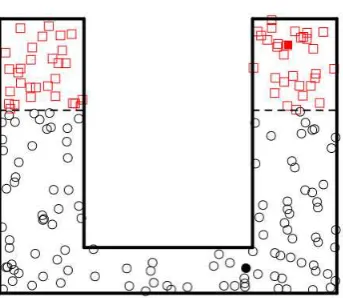
2) Connectedness of I0 and I1 is also critical. In a situation like the one shown in
Figure 1, the points in the connected component for which there is no point inDn
(represented as squares) will be classified as the circles by the algorithm. However, if I0 and I1 have a finite number of connected components and we have at least
one pair (Xi, Yi) ∈Dn in all of them withg∗(Xi) =Yi it is easy to see that the algorithm is consistent.
3) The uniform kernel can be replaced by any regular kernel satisfying c1IB(0,1)(u)≤K(u)≤c2IB(0,1)(u),
for some positive constantsc1, c2 and the results still hold.
4) We also assume that PX has a continuous density f with compact support S. If that is not the case, we can take a large enough compact set S such thatPX(Sc) be very small and therefore just a few data fromXl will be left out.
5) The following example shows that H4 is necessary. Indeed, suppose that U1 :=
X|Y = 1 ∼ U([a,1]) and U0 = X|Y = 0 ∼ U([0, a]) with 0 < a < 1, and
PX = aU0+ (1−a)U1 ∼U([0,1]). Unless that the training sample Dn contains
two points (X1,0) and (X2,1) withX1 andX2 close toa, semisupervised methods
will fail.
8
An Example
We end by illustrating with a simple example. We consider a semi–supervised problem with two classes{0,1}which are generated as follows. For the first class we generatel/3 points uniformly distributed on [−1,1]2 and keep only those in BdH(C, .15)∩[−1,1]
2,
where
Figure 1: The points labelled as 0 are represented with squares while the points labelled as 1 are represented with circles. Filled points belong toDn.
For the second class we generatelpoints in [−1,1]2and keep only those inBdH(C, .15)
c∩
[−1,1]2. The labelled training sample Dn consists on 5 points of each class, marked in magenta in Figure 2. We takek= 4,k= 8 and k= 12, with hl = 0.148 and l= 2400.
References
Aaron, C., Cholaquidis, A. and Cuevas (2017). Stochastic detection of some topological and geometric features. arXiv: https://arxiv.org/pdf/1702.05193.pdf
Agrawala, A.K. (1970). Learning with a probabilistic teacher. IEEE Transactions on Automatic Control, (19), 716–723
Azizyan, M., Singh, A., and Wasserman, L. (2013). Density-sensitive semisupervised inference. The Annals of Stastistics Vol. 41, No. 2, pp. 751–771.
Biau, G. and Devroye L. (2015). Lectures on the Nearest Neighbor Method Springer Series in Data Sciences..
Belkin, M. and Niyogi, P. (2004). Semi-supervised learning on Riemannian manifolds. Machine Learning 56pp. 209–239.
Ben-David, S., Lu, T. and Pal, D.(2008). Does unlabelled data provably help?. Worst-case analysis of the sample complexity of semi-supervised learning. In 21st An-nual Conference on Learning Theory (COLT). Available athttp://www.informatik. uni-trier.de/~ley/db/conf/colt/colt2008.html.
Chapelle, O., Sch¨olkopf, B. and Zien, A., eds. (2006) Semi-supervised learning. Adapta-tive computation and machine learning series. MIT
Cuevas, A. and Fraiman, R. (1997). A plug–in approach to support estimation Annals of Statistics 252300–2312.
Cuevas, A. and Rodr´ıguez-Casal, A. (2004). On boundary estimation. Adv. in Appl. Probab. 36340–354.
Federer, H. (1959) Curvature measures. Trans. Amer. Math. Soc.,93, 418–491.
Fralick, S.C. (1967) Learning recognize patterns without teacher.IEEE Transactions on Information Theory (13) 57–64.
Haffari, G. and Sarkar, A. (2007) Analysis of Semi-Supervised Learning with the Yarkowsky algoritm. In Proceedings of the 23rd Conference on Uncertainty in Ar-tificial Intelligence, UAI 2007. Vancouver, BC. July 19-22, 2007.
Lafferty, J. and Wasserman, L. (2007). Statistical analysis of semi-supervised regression. In Advances in Neural Information Processing Systems.20 pp. 801–808. MIT Press, Cambridge, MA.
Niyogi, P. (2008). Manifold regularization and semi-supervised learning: Some theoretical analyses. Technical Report TR-2008-01, Computer Science Dept., Univ. Chicago. Available at http://people.cs.uchicago.edu/~niyogi/papersps/ ssminimax2.pdf.
Penrose. M.D. (1999) A strong law for the largest edge of the minimal spanning tree. Annals of Probability. 27(1), 246–260.
Rigollet, P. (2007). Generalized error bound in semi-supervised classification under the cluster assumption. J. Mach. Learn. Res.8 pp. 1369–1392. MR2332435.
Scudder, H. J. (1965) Probability of error of some adaptive patter-recognition machines. IEEE Transactions on Information Theory, (11), 363-371.
Singh, A., Nowak, R. D. and Zhu, X.(2008). Unlabeled data: Now it helps, now it doesn’t. Technical report, ECE Dept., Univ. Wisconsin-Madison. Available at www. cs.cmu.edu/~aarti/pubs/SSL_TR.pdf.
Sinha, K. and Belkin, M. (2009). Semi-supervised learning using sparse eigenfunction bases. InAdvances in Neural Information Processing Systems 22(Y. Bengio, D. Schu-urmans, J. Lafferty, C.K.I. Williams and A. Culotta, eds.) pp. 1687–1695. MIT Press, Cambridge, MA.
Th¨ale, C. (2008). 50 years sets with positive reach. A survey. Surveys in Mathematics and its Applications 3, 123–165.
Walther, G. (1997). Granulometric smoothing. Ann. Statist.252273–2299.