Uniform Non-Exhaustive Search on Sparse
Reconstruction for Direction of Arrival Estimation
Koredianto Usman
Faculty of Electical EngineeringTelkom University;
School of Electical and Informatics Institut Teknologi Bandung
Email: [email protected]
Andriyan Bayu Suksmono
School of Electical and InformaticsInstitut Teknologi Bandung Email: [email protected]
Hendra Gunawan
Faculty of Mathematics and Science Institut Teknologi Bandung Email : [email protected]
Abstract—Direction of arrival estimation (DoA) using sparse reconstruction gives advantage on minimizing the number of re-quired samples. Among available sparse reconstruction schemes, angle sparsity has shown a favorable advantage as it requires fewer samples compare to other schemes. Previous researches on angle sparsity utilized an exhaustive scanning on every possible arrival angles. This technique leads to a problem of large sensing matrixA. The result presented in this paper proves that partial scanning (i.e. non-exhaustive search) also gives similar accurate result. The advantage of this scheme is smaller sensing matrix. In simulation, this scheme requires sensing matrix six times less than the exhaustive search with similar accuracy. Thus, this scheme is potential for practical application of DoA estimation based on sparse reconstruction.
I. INTRODUCTION
The development of compressive sensing (CS) has attracted considerable attention in recent decade. CS gives an alternative to classical Shannon-Nyquist sampling criteria for perfect construction. It was shown that sparse signal can be sampled at much lower sampling rate that the minimum Shannon-Nyquist sampling theorem. Sparse signal is defined as signal with few non-zero values while majority of the samples have zero values. Pioneers work in the field of CS are, among others, Donoho [1], Candes and Wakin [2], and Baraniuk [3]. With its advantage on small amount of samples, CS has been applied in various engineering applications, such as wireless sensors network, channel estimation, biomedical engineering, sonar, and radar applications ([4]).
In the radar area, especially in direction of arrival (DoA) estimation of incoming object, various CS schemes had been applied as alternative of classical DoA estimation algorithms, such as MVDR [5], MUSIC [6], and ESPRIT [7]. As far as CS is concerned, there are three main CS schemes that applied to the DoA estimation, namely: time sparsity ([8], [9]), space sparsity ([10], [11]), and angle sparsity ([12], [13]).
Time sparsity scheme based on an assumption that trans-mitted signal is sparse in time. The signalxis collected byM antennas ofN time snapshots to produce a block of M times
N size of input signal. Using block processing, each block of received signal of size is pre-multiplied by sensing matrix A (aM timesk matrix, with k<< N) to produce a smaller set of sensed signal. In the DoA estimation side, the compressed signal is reconstructed using CS reconstruction algorithms,
then DoA estimation is performed upon the reconstructed signal.
Space sparsity scheme is basically similar to the time sparsity. It is based on assumption that the signal received by each sensors (i.e. antennas) are similar to each others, thus can be assumed sparse as well. Signal reduction is performed by selecting sensing matrix Athat reduces dimension on sensors direction (i.e. a k times N matrix). The signal needs to be reconstructed before DoA estimation is performed. Compared to time sparsity, spase sparsity has less compression capability. Space sparsity, however, has advantage on robustness against noise. In addition, the space sparsty can be implemented directly by modifying hardware at the receiver side ([10] and [11]). Thus, no extra computation is needed.
Angle sparsity has a difference approach as the previous schemes. It does not compressed the received signal in time or space direction. However it assumes that the received signal is coming from a limited number of directions. Based on this, CS construction is performed using sensing matrix A taken from a set of antenna steering vectors. The CS formulation is composed from sensing matrix A, a sparse matrix s, and snapshots of received signal x. This CS construction can be represented by Eq.1.
A·s=x (1)
By using this approach, angle sparsity scheme has ad-vantage over time sparsity and angle sparsity, which are lesser samples. In addition, angle sparsity performs the CS construction and DoA estimation in single step. This technique was introduced by Gorotnitsky and Rao [12]. In the paper, they showed that one sample is sufficient to perform DoA estimation.
Given this advantage, angle sparsity is, however, less robust to the noise. Usman et al. [5] verified this condition and proposed improvement by using multi-snaps signal. In this multi-snaps scheme, the estimated DoA is determined by averaging over each samples. Stoica et al. [13] independently proposed covariance-based estimation technique (SPICE) in angle sparsity DoA. Their scheme also accommodates multi-snaps samples to improve robustness. As researchers mitigated the noise problem, angle sparsity has another weakness, which is large sensing matrix A. Usman et al. [14] and Stoica et al. [13] used exhaustive scan of possible angles (-900
to 900
Assuming angle scanning resolution as 0.50
, this produces sensing matrix A of size M times 360. If the number of antennas M is large, then this leads to CS reconstruction problem deal with large size matrix. Computation complexity increases correspondingly.
This paper proposes a solution to the exhaustive scanning problem by using a non-exhaustive scanning technique. The technique in principle is to reduce the scanning window into a narrower range. A pre-scanning technique is used to initially located the objects. After location of objects are pre-located, the next scanning is performed on narrow range around these objects. In the case of moving objects, the scheme can easily adapt the position by updating the searching window. We also proposed a tail scanning to further improve the accuracy of this non-exhaustive technique in case of a very narrow range of scanning window.
The presentation in this paper is arranged as follow: Section II discuss mathematical model and detail of the proposed scheme, Section III shows the simulation result and discussion, and finally section IV concludes this paper.
II. NON-EXHAUSTIVE SEARCH
A. Mathematical Model
We consider the set of M antennas arranged linearly with constant distance betwen antennas. This arrangement is called uniform linear array (ULA). Assumed that a source signal coming at angle θrelative to a reference line (Fig.1).
d
d
θ
l1
l2
l3
lM ∆
2∆
(M−1)∆
R
x1(t)
x2(t)
x3(t)
xM(t)
Fig. 1. Antennas arrangement in ULA with distancedbetween element
Assuming that the source is located at distance much larger than the size of the array, then the beam of signals arrived at each antennas can be considered parallel to each others. The difference of traveled distance of neighboring antenna is given by
∆ =d·sin(θ). (2)
This amount of distance corresponding to phase delay of
ψ= 2π
λ ·d·sin(θ) (3)
Collecting each received signal at each antennas, and write it in matrix form, we obtain
x= a·s+n (4)
In Eq.4,sdenotes the received signal at antennas’ input (p times N snapsmatrix;pis number of objects),x denotes the received signal after antennas (M timesN snapsmatrix),nis white gaussian noise, and a is array steering vector or array manifold. The steering vectora is expressed as
a=1 e−jψ e−j(M−1)ψT (5)
B. Compressive Sensing Formulation
The angle sparsity can be represented by Eq.1. Fig.?? clarifies the scheme into a detail structure.
a11
a21
aM1
a12
a22
aM2
a1p
a2p
aM p A
s1
s2
s3
sp
x1i
x2i
x3i
xM i
s x
a(θ1) a(θ2) a(θM)
steering vector at angleθi
Fig. 2. The CS construction of angle sparsity DoA
The sparse reconstruction is achieved by solving Eq.1 for sparse matrix s. Solving the equation for s is on the same time solving the DoA estimation problem, since location of non-zero element of s indicates the angle of arrival ([12]). However, since the number of equations is less then the number of unknowns, then Eq.1 leads to an ill-posed matrix problem. In other word, there are many set ofsthat fulfilled 1.
Back to the assumption the received signal is sparse in angle of arrival (i.e. in steering vector a), then the optimal solution is obtained by selecting the solution that minimize
l-norm of s ([2]). For sparse reconstruction, the appropriate norm is either l0 or l1-norm. Norm l1 is normally chosen for computation simplicity ([15]). The formal problem of CS reconstruction is, therefore, described by Eq.6
min ksk1 subject to A·s=x. (6)
In the case of noisy environment, which is common in telecommunication, the formulation of CS problem can be generalized by minimizing l1-norm on s, while constraining thel2-norm of difference between the estimation and the actual signal less than a certain threshold (ǫ). This formulation is written in Eq.7. This equation is called l1−l2 optimization problem (detailed discussion in [4] and references therein).
min ksk1 subject to kA·s−xk2< ǫ (7)
C. CS solver by convex programming
while l1-magic is developed by Candes and Romberg. CVX-programming is more generic to solve various convex program-ming problem. Thus, it is flexible. As a convex programprogram-ming tool, cvx-programming utilize some solver engine such as SDPT3 and SeDumi. To solve the CS problem as depicted in Eq.7, in CVX we write, for example:
begin_cvx
D. Uniform non-exhaustive searching
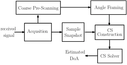
In order to reduce the computation complexity, we propose a uniform non-exhaustive searching on the DoA. At the beginning of operation, classical method such as MVDR is used to coarsely estimate the DoA. After the coarse location is determined, the scanning window is narrowed at next iteration. The center of scanning window is at the coarse DoA. The steering vectors of narrowed scanning window is updated as sensing matrix A. As the location of object is changed from time to time, it is also important to update the scanning window. The DoA of object is directly obtained from non-zero element of vectorsin each iteration.
Acqusition
Coarse Pre-Scanning Angle Framing
Sample CS
Fig. 3. Block diagram of proposed scheme
It is worth to note that the original scheme as proposed by Gorotnitsky and Rao utilizes a single snapshot ([12]). However we can extend the scheme by using multiple snapshots by extending column of vector x and column of vector s corre-spondingly (as also done in [14]). If the time duration of each snapshot is short enough, then we can assume that the object is still on its location, therefore we can do averaging on the value of every column of matrixsto obtain a robust estimate of the DoA.
In this paper, we propose two schemes of non-exhaustive scanning, i.e., scanning without tail scan and scanning with tail scan. Tail scan is an additional scanning at outside of the main scanning window. In the without tail scan, the scheme is suffered from the situation where cvx-programming is failed to converge, especially if main scanning window is too narrow. Thus, additional tail scan is useful to ensure the convergence of the cvx-programming. Fig.4 shows illustration of the exhaustive search, the uniform non-exhaustive search without tail scan, and the uniform non-exhaustive search with tail scan.
The are several techniques to update the scanning range. In this paper, we update the center of scanning window by
object object object
Fig. 4. Schemes illustration: a). exhaustive search b). uniform non-exhaustive search without tail scan, c). uniform non-exhaustive search with tail scan
aligning the center of the window to the object’s DoA. The higher and lower border of scanning range is adjust so that the maximum value is the median of the scanning range. The center aligning process is given by
θPmax =med([θmin, θmax]) (8)
In Eq.8,θPmax is the estimated DoA,θmin denotes lower
border of scanning angle, while θmax denotes the upper
border.
III. SIMULATIONRESULTS
To evaluate the performance of the proposed scheme, we performed a computer simulation. In this simulation, a single source of object is moving from 300 to 600 with angular speed of 1.40
per second. This angular speed is equivalent to commercial airplane moving at linear speed of 1,000 kmph at altitude 10 km (about 30,000 feet) above the ground. The object is assumed to move circularly at a constant distance to the receiver. As the receiver, we use ULA of 12 antennas. The distance between antenna elements is a half of the signal wavelength. We assume that the signal strength as compare to noise (SNR) is 10 dB. At the initial operation of the DoA estimation, a coarse DoA is performed using MVDR algorithm. The signal spectrum as function of scanning angle
θ is given by: angle θ, and R−xx1 is inverse of covariance matrix of received
signalx. Coarse DoA is taken at an angle whose DoA power spectrum is maximum.
After coarse DoA is determined, the non-exhaustive al-gorithm is performed by limited the scanned signal around this maximum power spectrum. We performed simulation on exhaustive scanning (scanning window −900
to 900
), and then non-exhaustive search by reducing scanning window from
−300
to900
and00
to900
. A actual position of object is used as reference. As performance parameter, we use mean absolute error (MAE) of each scheme. MAE is defined as:
M AE = 1
Actual angle of arrival at timei is denoted by θai, while
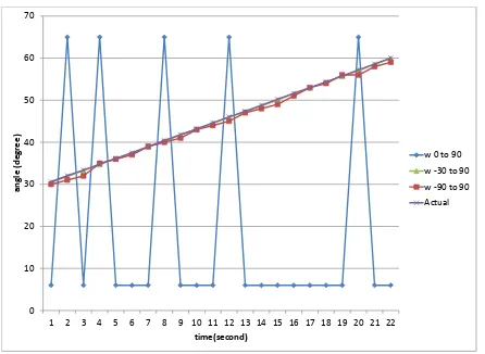
indicates a better estimate. Fig. 5 shows the simulation result. As observed in the figure, the actual position of the object is linearly changed by time. The exhaustive search performs well in tracking the object’s DoA with MAE is 0.6. The narrower scanning of−300
to900
performs slightly worse (with MAE value of 1.6). This is because narrower scanning window has less information for cvx-programming to iterate.
0
Fig. 5. Comparison of exhaustive search (-900 to 900) and non-exhaustive
searches
The situation is different in the case of searching range00
to900
. The estimated angle is incorrectly in off positions. The estimated angles are bounced back between50
and650
. This phenomena indicates failures of cvx-programming to give a converge solution. The bounce back values, indicates that the cvx iteration is trapped within these values.
To improve this situation, we add a few additional scanning outside the window scanning range (i.e. the tail scanning). There are several methods to add these tail scanning. In the simulation, we tried two methods, which are, uniform tail scan and random tail scan. In the uniform tail scan, we scan in additional 12 scanning directions which are uniformly separated at 200
to each others. Random tail scanning, on the other hand, scattered these 12 scanning directions randomly. Fig. 6 shows the simulation result of these tail scanning. In this simulation, window scanning range is00
to900
.
As shown in Fig. 6, the performance of non-exhaustive searches, both uniform tail scan and random tail scan, improve accuracy of estimation. There is, however, an off-position which took place at the time 11 (uniform scan tail) and 15 (random scan tail). This off-position statistically can take place at any time. This indicate that cvx-programming failed to give a convergence solution. This off-position is can be easily detected and removed. Interpolation of neighbors value can be used to substitute these off-positions.
As the tail scan has successfully improve the non-exhaustive search, we further narrowing the scanning window from 300
to 600
. This scanning window is exactly the same to the track of the object. Here again, we simulate both uniform tail scanning and random tail scanning. Fig. 6 show the simulation result. The performance of exhaustive search is
-100
Fig. 6. Comparison of uniform and random tail scan exhaustive search
also included as a reference. In the depicted figure, we observe that non-exhaustive search with uniform tail scan and random tail scan performed as good as exhaustive search. Uniform and random tail scan gave MAE of 0.81 and 0.56 respectively. Exhaustive search, on the other hand gave MAE of 0.61.
If we compare the computation complexity, non-exhaustive search has smaller sensing matrix A, which is M times 30 for non-exhaustive compared to M times 180 for exhaustive search. In other word, in this simulation, non-exhaustive search has about 150M less computation compared to the exhaustive search. Here,M is number of antennas in the array.
0
Fig. 7. Comparison of exhaustive search and non-exhaustive search using uniform and random tail scan. Off-position is removed by interpolation
IV. CONCLUSION
window. The main limitation of this scheme, especially as combined with the cvx-programming, is that it does not converge if the window range is narrow. We show also that adding tail scan can mitigate this problem. Two methods of tail scans were tested in this paper, which are uniform tail scan and random tail scan. These two methods perform very closed to the exhaustive search in term of accuracy. Main advantage of this schemes is smaller sensing matrix A, which means a faster computation. This advantage may add practicality of this scheme for actual implementation. Mathematical background for tail scan, however, is still necessary to be explored in future research.
ACKNOWLEDGMENT
The authors would like to thank to Yayasan Pendidikan Telkom and Indonesian Ministry of Education and Culture for their support on this study.
REFERENCES
[1] D. L. Donoho, “Compressed sensing,”IEEE Transactions on Informa-tion Theory, vol. 52, no. 4, April 2006.
[2] E. Candes and M. Wakin, “An introduction to compressive sampling,” IEEE Signal Processing Magazine, vol. 25, no. 2, pp. 21–30, March 2008.
[3] R. Baraniuk, “Compressive sensing,”IEEE Signal Processing Maga-zine, vol. 24, Jul 2007.
[4] K. Hayasi, M. Nagahara, and T. Tanaka, “A users guide to compres-sive sensing for communications systems,”In IEICE Transaction on Communication, vol. E96-B, no. 3, pp. 685–712, March 2013. [5] J. Capon, “High-resolution frequency-wavenumber spectrum analysis,”
Proceedings of the IEEE, vol. 57, no. 8, pp. 1408–1418, Aug 1969. [6] R. Schmidt, “Multiple emitter location and signal parameter estimation,”
IEEE Transactions on Antennas and Propagation, vol. 34, no. 3, pp. 276–280, Mar 1986.
[7] R. Roy, A. Paulraj, and T. Kailath, “Estimation of signal parameters via rotational invariance techniques esprit.”Proceeding of IEEE Military Communications (MILCOM) Conference - Communications, vol. 3, Oct 1986.
[8] A. C. Gurbuz and J. H. McClellan, “A compressive beamforming method,”Proceeding of the IEEE International Conference on Acous-tics, Speech and Signal Processing, 2008.
[9] J. M. Kim, O. K. Lee, and J. C. Ye, “Compressive music: Revisiting the link between compressive sensing and array signal processing,”IEEE Transactions on Information Theory, Vol. 58, No. 1, January 2012, 2012. [10] Y. Wang, G. Leus, and A. Pandharipande, “Direction estimation using compressive sampling array processing,” inProceeding of IEEE SSP, 2009.
[11] Y. Wang, A. Pandharipande, and G. Leus, “Compressive sampling based mvdr spectrum sensing,”Proceeding of IAPR, 2010.
[12] I. F. Gorodnitsky and B. D. Rao, “Sparse signal reconstruction from limited data using focuss: A re-weighted minimum norm algorithm,” IEEE Transactions on Signal Processing, vol. 45, no. 3, March 1997. [13] P. Stoica, P. Babu, and J. Li, “Spice: A sparse covariance-based
estimation method for array processing,”IEEE Transactions on Signal Processing, vol. 59, no. 2, pp. 629–638, Feb 2011.
[14] K. Usman, A. B. Suksmono, and H. Gunawan, “Peningkatan kinerja skema estimasi arah kedatangan sinyal dengan compressive sensing sparsitas sudut dan sampel multisnap,”Inkom Journal, vol. 8, no. 1, pp. 21–27, May 2014.
[15] J. Romberg. (2005) l1-magic. [Online]. Available: http://users.ece.gatech.edu/ justin/l1magic/