The di
!
erence between the managerial and mathematical
interpretation of sensitivity analysis results in
linear programming
Tama
H
s Koltai
!,
*
, Tama
H
s Terlaky
"
!Technical University of Budapest, Department of Industrial Management and Economics, H-1521 Budapest, Hungary
"Delft University of Technology, Faculty of Information Technology and Systems, Department of Technical Mathematics and Informatics, P.O. Box 5031, 2600 GA Delft, The Netherlands
Received 7 December 1998; accepted 28 March 1999
Abstract
This paper shows that managerial questions are not answered satisfactorily with the mathematical interpretation of sensitivity analysis when the solution of a linear programing model is degenerate. Most of the commercially available software packages provide sensitivity results about the optimality of a basis and not about the optimality of the values of the decision variables. The misunderstanding of the shadow price and the validity range information provided by a simplex based computer program may lead to wrong decision with considerable "nancial losses and strategic consequences. The paper classi"es the most important types of sensitivity information, graphically illustrates degeneracy, and demonstrates its e!ect on sensitivity analysis. A production planning example is provided to show the possibility of faulty production management decisions when sensitivity results are not understood correctly. Finally the recommenda-tions for the users of linear programing models and for software developers are provided. ( 2000 Elsevier Science B.V. All rights reserved.
Keywords: Linear programming; Sensitivity analysis; Production management
1. Introduction
Linear programing (LP) is one of the most exten-sively used operations research technique in pro-duction and operations management [1]. As a result of the development of computer technology and the rapid evolution of user friendly LP
soft-*Corresponding author. Tel.:#36-1-463-2456; fax: #36-1-463-1606.
E-mail address:[email protected] (T. Koltai)
ware, every operation manager can run an LP software easily and quickly on a laptop computer. Although solving LP models is now accessible for everybody, the interpretation of the results requires a lot of skill. Most of the management science and OR textbooks pay special attention to sensitivity analysis, and the problems of degeneracy, but sensi-tivity analysis under degeneracy is rarely discussed. Commercially available software do not give enough information to the user about the existence and the consequences of these, very common,
`special casesa. In practice, managers very fre-quently misinterpret the LP results which may lead
to erroneous decisions and to important "nancial and/or strategic disadvantages.
Several papers have addressed this issue. Evans and Baker draw the attention to the consequences of the misinterpretation of sensitivity analysis results in management. They illustrate their point with a simple example and list some published cases in which the erroneous interpretation of sensitivity analysis results is obvious [2]. Aucamp and Steinberg [3] also warn that shadow price analysis is incorrect in many textbooks, and that the shadow price is not equal to`the optimal solu-tion of the dual problem''when the obtained opti-mal solution is degenerate. They present some examples of shadow price calculations by com-mercial packages. AkguKl [4] re"nes the shadow price de"nition of Aucamp and Steinberg, and introduces the negative and positive shadow prices for the increase and the decrease of the RHS elements. Greenberg [5] shows that very frequently practical LP models have a netform structure, and netform structures are always de-generate. He illustrates sensitivity analysis of netform type models by one of the Midterm Energy Market Model of the U.S. Department of Energy. Gal [6] summarizes most of the critics concerning sensitivity analysis of LP models and highlights some important research directions. Rubin and Wagner [7] illustrates the traps of the interpretation of LP results by using the in-dustry cost curve model in a tutorial type paper written for managers and instructors. Jansen et al. [8] explain the e!ect of degeneracy on sensitivity analysis by using a transportation model, and present the shortcomings of the most frequently used LP packages. They also show how complete, correct sensitivity analysis can be done. Wendell [9,10] also pays special attention to the correct and practically useful calculation of sensitivity in-formation. The biggest problem is not that opera-tions researchers are unaware of the di$culties of sensitivity analysis. This issue is discussed thor-oughly in the scienti"c literature (see for example [6,10,11]) and a complete, mathematically correct treatment of sensitivity analysis is presented by Jansen et al. [8], and by Roos et al. [12]. Practice, however, shows that the problem is not widely known among the LP users, and the available
commercial software packages are not helpful in recognizing the di$culties.
The main objective of this paper is to explain the di!erence between the managerial questions and the traditional mathematical interpretation of sen-sitivity analysis. In the"rst part of the paper basic
de"nitions are introduced, the most important
types of sensitivity information are classi"ed, and degenerate LP solutions are illustrated graphically. In the second part a production planning prob-lem is used to demonstrate the consequences of incorrect interpretations of the provided sensi-tivity information. Finally, some recommenda-tions are made for both practitioners and software developers.
2. Basic de5nitions and concepts
Every LP problem can be written in the follow-ing standard form:
min
x
McTxDAx"b,x*0N, (1)
whereAis a givenm]nmatrix with full row rank
and the column vectorbrepresents the right-hand side (RHS) terms and the row vectorcTrepresents the objective function coe$cients (OFC). Problem (1) is called theprimal problemand a vectorx*0 satisfyingAx"bis calleda primal feasible solution. The objective is to determine those values of the vectorxwhich minimize the objective function. To every primal problem (1) the following problem is associated:
max
y
MbTyDATy)cN. (2)
Problem (2) is called thedual problemand a vector
ysatisfyingATy)cis called adual feasible solution. For every primal feasible x and dual feasibleyit holds thatcTx*bTyand the two respective objec-tive function values are equal if and only if both the solutions are optimal.
implemented sensitivity analysis is based always on the simplex method. The simplex procedure selects a basis of the matrix Ain every step, the selected
basis solutionis calculated and the optimality
cri-teria is checked. To de"ne the optimal basis solution some preparation is needed. Let B be a set of m indices, and A
B be the matrix obtained
by taking only those columns of Awhose indices are inB. IfA
Bis a nonsingular matrix then by using
the vector x
B"A~1B ba basis solution can be
de-"ned as
x
j"
G
(x
B)j ifj3B,
0 otherwise. (3)
If in additionx
B*0 holds thenxis called aprimal
feasible basic solution. The variables with their
index inBare thebasicvariables, the others are the
nonbasicvariables. Dual variables can be associated
to any basisA
Bas follows:
y"(A~1B )Tc
B. (4)
Ifc!ATy*0 thenyis a feasible solution for the dual problem and is called thedual feasible basic
solution. If the basis A
B is both primal and dual
feasible, thenA
Bis anoptimal basis, and the
corre-sponding basic solutionsxandyareoptimal basis
solutions for the primal and the dual problems,
respectively. It might happen, that a basis gives an optimal primal solution, but the related dual basis solution is dual infeasible. Such a basis is called the
primal optimal. Analogously, when a basis gives
a dual optimal solution, but the related primal solution is infeasible, then the basis is called the
dual optimal.
Sometimes the optimal basis is not unique, more than one basis may yield an optimal solu-tion either for the primal or for the dual problem or for both. This is called degeneracy and occurs in almost all practical problems. Formally, a basis is called primal degenerate when there are variables with zero value among the basis variables and it is called dual degenerate when some dual slack variables s
j"cj!(ATy)j, not belonging to
the basis indices B, are zero. In general, if a basis is either primal, or dual, or from both sides degen-erate then we simply say that it is degendegen-erate. In case of degeneracy many optimal solutions exist
that are not basis solutions, e.g. interior point methods provide the so-calledstrictly
complement-ary optimal solutions. Strictly complementary
opti-mal solutions are the optiopti-mal solutions x,ysuch thatx#(c!ATy)'0.
Very frequently the basic parameters of an LP model changes (e.g. cost coe$cients, resource ca-pacities, etc.) and it would be important to know if any action on behalf of the decision maker is required as a consequence of these changes. Sensitivity analysis can help to answer this ques-tion if it is applied correctly. The objective of sensitivity analysis is to analyze the e!ect of the change of the objective function coe$cients (OFC) and the e!ect of changes of right-hand side (RHS) elements on the optimal value of the objective function, and the validity ranges of these e!ects. Depending on how this analysis is performed, three types of sensitivities are cal-culated:
f Type I sensitivity: Type I sensitivity determines
those values of some model parameters for which a givenoptimal basisremains optimal. Sensitivity analysis of the optimal basis for the OFC ele-ments determines within which range of an OFC the current optimal basis remains optimal and what is the rate of change (directional derivative) of the optimal objective function value when the OFC changes within this range. In case of the RHS elements the question is, within which range an RHS element can change so that the current optimal basis stays optimal, and what is the rate of change (shadow price) of the optimal objective function value within the determined interval.
misleading for decision makers, if the given in-formation is not interpreted correctly.
f Type II sensitivity: Type II sensitivity determines
those values of some model parameters for which
the positivevariables in a given primal and dual
optimal solution canremain positive, and the zero
variables remain zero, i.e. the same activities re-main active. More accurately, we have an opti-mal solution (not necessarily basis solution)
xwith its support set supp(x)"MiDx
i'0N. We
are looking for those model parameters, for which an optimal solution (basis or not basis) exists with precisely the same support set. Sen-sitivity analysis of a given optimal solution for an OFC determines within which range of the OFC an optimal solution with the same support set exists and what is the rate of change (directional derivative) of the optimal objective function value when the OFC changes within this range. In case of the RHS elements the question is, within which range a RHS ele-ment can change without the change of the sup-port set of the optimal solution, and what is the rate of change (shadow price) of the optimal objective function value within the determined interval.
Contrary to Type I sensitivity, Type II sensitivity depends on the produced optimal solution, but not on which basis } if any } represents the given optimal solution.
f Type III sensitivity: Type III sensitivity
deter-mines those values of some model parameters for whichthe rate of change of the optimal objective
function value is the same. Roughly speaking
sensitivity (and range) analysis means the analy-sis of the e!ects of the change of some problem data, in particular an objective coe$cientc
j or
right-hand side coe$cientb
j. Let us assume that
either c
j#c orbi#b is the perturbation. It is
known that the optimal value function is a piece-wise linear function of the parameter change (see for example [9,11]). In performing Type III sen-sitivity analysis one wants to determine the rate of the change of the optimal value function and the intervals within which the optimal value function changes linearly.
Type III sensitivity information is independent of the solution obtained, it depends only on the prob-lem data and on which OFC or RHS eprob-lement is changing.
As a short recapitulation observe that:
f Type I sensitivity depends on the type of optimal
basis solution produced and on the type of opti-mal basis found to represent the given optiopti-mal basis solution.
f Type II sensitivity depends on the type of
opti-mal solution (not necessarily a basis solution) produced. If eventually it is an optimal basis solution, then Type II sensitivity information is independent of the basis representation of the found optimal basis solution.
f Type III sensitivity is independent of the type of
optimal solution produced, and it is also inde-pendent of how the optimum is represented. It depends only on the problem data.
The calculation and importance of the three di! er-ent sensitivity information depends on the type of optimum solution produced by the LP solver. Most of the LP solvers used for small and medium size problems are based on some versions of the simplex method and they provide anoptimal basis solution. Other solvers, typically used for (very) large scale problems are based on interior point methods and they provide an interior (i.e. strictly complement-ary) optimal solution. To distinguish among the three type of sensitivities is necessary because of the existence of degeneracy. The following cases can be observed:
f When the optimal solution is neither primal
nor dual degenerate, all the three types of sensi-tivities are the same, since there is a unique optimal solution with a unique optimal basis. In this case the sensitivity analysis output of the commercially available software packages pro-vide reliable, useful information for decision making.
f When the optimal solution isonly primal
degen-erate, a unique primal optimal solution exists.
di!erent since there are di!erent Type I sensitiv-ity information for all the optimal basis. One important case is when the increase, and the decrease of an RHS parameter results in di!erent rate of changes, i.e. the optimal value function at the current point is not di!erentiable. Due to this fact the introduction of the right and left side shadow prices and their respective sensitivities [3] was needed. Type II and Type III sensitivity information for the RHS elements are split into two parts: the left and right side sensitivities. The left and right linearity intervals of the optimal value function provide the Type III information. When the left and right side shadow prices are identical, then only one interval is given. Type II and Type III sensitivity information for an OFC are identical in the case when the solution is only primal degenerate.
f When the optimal solution isonly dual
degener-ate, several di!erent primal optimal basis and nonbasis solutions may exist with di!erent sup-port sets, while the dual optimal solution is unique. In this case Type I and Type II sensitivi-ties at each alternative primal optimal basic solu-tions are identical, but Type II sensitivities can be calculated from the nonbasic solutions as well. Type II sensitivity is interested only in the optimal solutions belonging to the same support sets, therefore, Type III sensitivity may be di! er-ent from the Type II sensitivities of each optimal solutions, except at the strictly complementary ones.
f When the optimum is both primal and dual
de-generate, then all the three types of sensitivities
may be di!erent. In this case each optimal basis of each optimal basis solution may have a dif-ferent Type I sensitivity information. Optimal solutions with di!erent support sets may have di!erent Type II sensitivities and can be exam-ined at nonbasis solutions too. As it is known, Type III sensitivity information is uniquely determined, it is independent of the optimal solution obtained. Typically, the intervals pro-vided by Type I and Type II sensitivities are subintervals of the Type III sensitivity inter-vals. The rates of changes produced by Type I and Type II either coincide with Type III in-formation or are useless, their validity (as a
sub-di!erential) is restricted to the current point only.
f When the current optimum is a strictly
com-plementaryoptimal solution, e.g. when the
prob-lem was solved by interior point methods, then Type II and Type III sensitivities are the same. When the optimal solution at hand is not a strictly complementary one, Type II and Type III sensitivities might be di!erent. In this case the left and right intervals of Type II sensitivities are possibly subintervals on the Type III sensitivity intervals.
An important question is, when the di!erence between Type II and Type III sensitivities is impor-tant for the decision maker. If the decision maker implements an optimal solution, then in many situ-ations, the important information is the sensitivity of theimplemented optimal solution (Type II sensi-tivity). For example if an optimal production plan, determined by LP, is already running, then the important question is how the change of certain costs, or the change of a machine capacity in# uen-ces the implemented plan. If the question is, how much an RHS element can be increased with the same consequences, and independently of the pos-sible change of an optimal solution, then it is a Type III sensitivity question. For example if a machine capacity can be increased economically at the calculated shadow price, important informa-tion can be how much the capacity can be increased economically in total. It is possible that di!erent production plans (di!erent optimal solutions, espe-cially when optimal basis solutions are imple-mented) belonging to di!erent capacities increase, but all capacity extensions are made with the same marginal bene"ts.
sensitivity information are identical in this case, because the change of the support set of a strictly complementary optimal solution is in one to one correspondence with the linearity intervals of the optimal value function [12].
The di!erent questions of Type I, Type II and Type III sensitivity can be made transparent when one observes that in the case of degeneracy optimal solutions might exist that are neither the basis solutions nor strictly the complementary solutions. In such a case all the three sensitivities might be di!erent. Type I has no sense when no optimal basis is at hand. Type II depends on the current solution while Type III does not. The di!erent type of solutions of an LP problem are illustrated in Fig. 1. Let us assume that the set of the feasible solutions is the unit cube and the objective is to maximizex
3, that is,
max (x
3)
subject to
x
1 #s1 "1,
x
2 #s2 "1,
x
3 #s3"1,
(5)
x
1,x2,x3,s1,s2,s3*0.
Fig. 1. Graphical illustration of the di!erent type of LP solu-tions.
In this case the solution P
1"(0, 0, 1; 1, 1, 0) is
an optimal basis solution with the basis given by the variables (s
1,s2,x3). The solution P2"
(1/2, 1/2, 1; 1/2, 1/2, 0) is a strictly complementary optimal solution, while the solution P
3"
(0, 1/2, 1; 1, 1/2, 0) is an optimal solution which is neither a basis nor a strictly complementary solution.
As a summary it can be stated that in case of degeneracy, commercial packages do not pro-vide the sensitivity information useful for the decision maker (note that in practice almost all problems are degenerate). They give answer to a less ambitious question. They provide in-formation about the interval of a parameter value within which the current optimal basis re-mains optimal, and at what rate the change of the parameter varies the optimal function value in that interval (Type I sensitivity). This answer is intimately related to the optimal basis ob-tained by the simplex solver. In case of degeneracy many di!erent optimal basis exist, thus many di!erent ranges and rates of changes might be obtained. To obtain the true Type III sensitivity information about the change of the value of the OFC and RHS elements one needs extra e!ort. In fact one has to solve some subsidiary LPs for deter-mining linearity intervals, and left and right deriva-tives of the optimal value function. In case of strictly complementary solutions provided by IPM solvers Type II and Type III sensitivities co-incide for some speci"c solutions. In all other cases they might be di!erent. The decision maker has to determine if Type II or Type III sensitivity is im-portant for a certain problem, and LP software packages should assist to obtain those information easily.
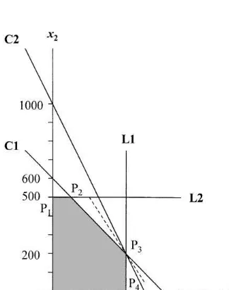
3. Graphical illustration of the problem of sensitivity analysis
problem:
max (12x
1#10x2)
subject to
(C1) x
1 #x2)600,
(C2) 2x
1#x2)1000,
(L1) x
1 )400,
(L2) x
2)500,
(6)
x
1*0,x2*0.
The feasible set and the solution of problem (6) can be seen in Fig. 2. The two constraints (C1) and (C2) and the upper bounds onx
1andx2(L1) and (L2)
are represented as half spaces. The boundary of these spaces with the corresponding labels are de-picted in the "gure. The intersection of these half spaces is represented as a shaded area, which con-tains all the primal feasible solutions. The objective function (iso-pro"t line) is drawn as a straight dashed line. The objective function touches the shaded area at pointP
3, therefore the unique
opti-mal solution is atx
1"400 and x2"200.
In order to transform problem (6) into the stan-dard form, indicated by problem (1),slackvariables
(denoted by s
i,i"1,2, 4) are introduced for all
Fig. 2. Graphical illustration of the prototype problem.
the constraints, and the objective function is changed to have a minimization problem. The problem in the standard form is as follows:
min (!12x
1!10x2)
subject to
(C1) x
1 #x2#s1 "600,
(C2) 2x
1#x2 #s2 "1000,
(L1) x
1 s3 "400,
(L2) x
2 #s4"500,
(7)
x
1,x2,s1,s2,s3,s4*0.
Problem (7) shows that A is a 4]6 matrix with
rank equal to 4. The values of the slack variables at
P
3are the following:
s
1"0;s2"0;s3"0;s4"300.
Since at P
3 there are three nonzero variables
(x
1,x2ands4) and the rank of the matrixAis 4, the
optimal solution is degenerate. This can be seen in Fig. 2. The pointP
3is the intersection of three lines
(the boundary of (C1), (C2) and (L1)). Two lines would be enough to determine the location of a point in a two-dimensional space, thereforeP
3 is
over determined. Even if we remove any one of (C2), or (L1), the pointP
3 remains the only
opti-mal solution. This over determination of the optimal point is a graphical illustration of primal degeneracy.
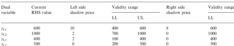
Let us see the consequences of degeneracy on sensitivity analysis. The shadow prices and the cor-responding validity ranges for the optimal solution, calculated with the help of Fig. 2, are given in Table 1. The change of an RHS element is repre-sented by a parallel shift of the corresponding line in Fig. 2.
If the RHS of any of these constraints are de-creased, then the left side shadow prices are ob-tained for each of the constraints respectively (column three of Table 1). The optimal pointP
3is
at the intersection of constraints (C1), (C2) and (L1). The decrease of any of the RHS of these constraints results in the movement of the optimum point,P
3,
Table 1
Shadow prices and validity ranges of the optimal values Dual
variable
Current RHS value
Left side shadow price
Validity range Right side shadow price
Validity range
LL UL LL UL
y
C1 600 10 400 600 8 600 750
y
C2 1000 2 700 1000 0 1000 R
y
L1 400 2 100 400 0 400 R
y
L2 500 0 200 500 0 500 R
does not a!ect the location ofP
3its shadow price is
zero. (C1) can be moved toP
4, (C2) and (L1) can be
moved to P
2 with the same shadow price value.
(L2) can be moved to P
3 without a!ecting the
objective function value. The corresponding lower limits (LL) are given in the fourth column of Table 1. In case of left side shadow prices the upper limits (UL) are equal to the current values of the RHS elements ("fth column of Table 1). If the RHS of any of these constraints are increased, then the right side shadow prices are obtained for each of the constraints, respectively (column six of Table 1). In case of constraints (C2) and (L2) the increase of the right-hand side values do not a!ect the location of the optimum point, because (C1) and either (C2) or (L1)"xes its place. Therefore the corresponding right side shadow prices are equal to zero. When the right hand side of (C1) is increased, then the optimum point will stay at the intersection of (C1) and (C2) and the shadow price will be equal to 8. Since (L2) does not a!ect the location of P
3 its
shadow price is also zero. In case of right side shadow prices the lower limits (LL) are equal to the current values of the RHS elements, while the upper limits (UL) are determined by the geometrical properties of the solution space. When (C1) is moved upward the intersection of (C1) and (C2)
P
3moves upward as well. WhenP3reaches (L2),
then the move of (C1) does not a!ect the location of
P
3any more, and the shadow price turns into zero.
The RHS value at this point is the UL of the sensitivity range, and it is equal to 750. The UL of all the other constrains are equal to in"nity.
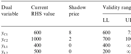
Table 2 shows the shadow prices and their valid-ity ranges found by the STORM computer package
Table 2
Shadow prices and validity ranges at the optimal basisB
1
Dual variable
Current RHS value
Shadow price
Validity range
LL UL
y
C1 600 10 400 600
y
C2 1000 0 1000 R
y
L1 400 2 100 400
y
L2 500 0 200 R
at the optimal basisB
1"M1, 2, 3, 6N. It can be seen
that at this basis the left side shadow prices and validity ranges were provided for constraints (C1) and (L1), and the right side shadow price and valid-ity range was found for the constraint (C2). Table 3 contains the shadow prices and their validity ranges found at the optimal basisB
2"M1, 2, 5, 6N.
At this basis the right side shadow prices and valid-ity ranges were provided for constraints (C1) and (L1), and the left side shadow price and validity range was found for the constraint (C2). The left and right side shadow prices for constraint (L1) are identical, and its correct value and validity range was found in both optimal basis as seen in the last rows of Tables 2 and 3.
Table 3
Shadow prices and validity ranges at the optimal basisB
2
Dual variable
Current RHS value
Shadow price
Validity range
LL UL
y
C1 600 8 600 750
y
C2 1000 2 700 1000
y
L1 400 0 400 R
y
L2 500 0 200 R
point, di!erent basis is considered, that is, di!erent sets ofBin (3) may lead to the same basis solution. This is the case atP
3, where Table 2 was calculated
with the help of a basis containing columns 1, 2, 4 and 6, and Table 3 was calculated with the help of a basis containing columns 1, 2, 5 and 6 of problem (7).
The main problem of RHS sensitivities in the prototype problem is that in case of a degenerate primal optimal solution the dual problem has no unique solution. Di!erent bases belonging to the same optimal solution provide di!erent shadow prices and validity ranges. Tables 2 and 3 show that the results provided by the two optimal bases are mixtures of the left side, right side and full shadow prices and validity ranges. The complete Type III information, similar to Table 1, is not given at any of the basis. It depends on the computer code at which basis, among the many optimum ones, the program stops. Di!erent commercially available software may report di!erent RHS sensitivities for the same problem [8]. All these results are correct mathematically, because they describe the validity of an optimal basis (Type I sensitivity), but are not useful for managerial decisions, because they do not re#ect the validity of thepositivity status of the
decisionvariables at optimality(Type II sensitivity),
and do not characterize the validity range of the
left/right marginalvalues(Type III sensitivity). The
correct RHS information, which refers to the rate of change of the optimal objective value, and the range where these rates are valid are given in Table 1. The Type II sensitivity of the RHS ele-ments are given in Table 1, in which for
y
C1,yC2,yL1, the left and right side sensitivities are
Type III information as well for two di!erent
Table 4
The increase of the objective function by a unit increment of the RHS elements
RHS elements Rate of change of the objective function
Validity range
C1 10 400)*b
C1)600
C2, L1 2 400)*b
L1)600
*b
C2"*bL1
linearity intervals. For y
L2, the Type II and Type
III sensitivity informations are identical.
It can be seen in Table 1 that most of the right-side shadow prices are zero. An interesting question is, how the optimal objective function value can be increased by the simultaneous increase of those RHS elements which have a zero shadow price. This question is equivalent to the problem of in-creasing the capacity of bottleneck resources of production systems. Fig. 2 shows that the RHS of (C1) can be increased alone, but the RHS of (C2) and (L1) need to be increased simultaneously. This information is summarized in Table 4. The opti-mum value of the objective function increases by 10 if the RHS of (C1) is increased by one unit. This is true within the interval [400, 600]. When the RHS of (C2) and (L1) are simultaneously increased by one unit, the change of the objective function value is 2 and the validity range is a line segment in a two-dimensional space, given in the last window of Table 4.
Since the objective function coe$cient sensitivity of the primal problem is the same as the RHS sensitivity of the dual problem, all what was said of the RHS is valid for the objective function coe$ -cients as well. Graphically the change of an OFC can be represented by the change of the slope of the line of the objective function. In Fig. 2 the optimal solution of problem (7) isP
3as long as the objective
function line stays between (L1) and (C1). The cor-responding sensitivities are given in Table 5. These data coincide with the sensitivities provided by the STORM computer package when the optimum was calculated at the basisB
1. The results provided
at the basisB
2are given in Table 6. The intervals
Table 5
Objective function coe$cient sensitivities and rate of change at the optimal basisB
1
Objective function coe$cient
Current value
Validity range Rates of changes
LL UL
c
1 12 10 R 400
c
2 10 0 12 200
Table 6
Objective function coe$cient sensitivities and rate of change at the optimal basisB
2
Objective function coe$cient
Current value
Validity range Rates of changes
LL UL
c
1 12 10 20 400
c
2 10 6 12 200
and 6 show the rate of changes of the optimum value function. The identical rate of changes of the respective coe$cients in both optimal basisB
1and
B
2indicate that the optimal solution is not a dual
degenerate. This is also clear from Fig. 2 since the optimal solution is unique.
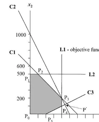
Fig. 3 illustrates a slight modi"cation of the sample problem. A new constraint ((C3):x
1!2x2
)200) is added to the problem and the objective function is also modi"ed (min[!12x
1!0x2]). In
this case the optimal objective function coincides with constraint (L1), and all the points in the inter-val [P
3,P4] are optimal. Consequently all the basis
at P
3 and the basis at P4 are optimal and the
optimal solution is both primal and dual degener-ate, and we expect di!erent Type I, Type II and Type III sensitivities. Let us consider now the shadow price and sensitivity range of the RHS of constraint (L1). It can be seen that as long as (L1) increases or decreases the shaded area the shadow price is equal to 12. This is true between points
P
0and P@ and corresponds to the RHS values of
(L1) in the interval [0, 440], which is the Type III sensitivity information for the RHS of (L1). If,
Fig. 3. Graphical illustration of the modi"ed prototype problem.
however, the problem is solved by a computer code of the simplex method, then depending on the basis found by the program, the following intervals can be obtained: [100, 400], [200, 440], [400, 440]. There are four di!erent Type I sensitivities. In this
modi"ed example the left and right-hand side
shadow prices are equal, and there are two di!erent Type II sensitivities for the two optimal basis solu-tions at P
3 and P4, which are [100, 440] and
[200, 440] respectively.
Finally let us take a strictly complementary solution of the modi"ed problem found by an IPM solver. On the P
3}P4 line segment the
point x
1"400, and x2"150 can be such an
optimum. For this solution Type I sensitivity has no sense because this is not a basis solution, and Type II and Type III sensitivities coincide, because this is a strictly complementary optimal solution. On the interval [0, 440] of the RHS of (L1) we always have solutions where bothx
1and
x
2 are positive while (L1) is the only active
con-straint.
several results are either incomplete or irrelevant from the point of view of the information required by a decision maker.
4. Illustration of the problems of degeneracy in a production planning model
Production planning is one of the most impor-tant application areas of linear programing. Either directly, as individual planning models, or indirect-ly, as part of a complex production planning and control system, linear programs are run and their results used for production management decisions. In most of the cases sensitivity analysis is more important than the optimum itself. On one hand, the exact result of an LP model can be implemented very rarely in practice, but small modi"cations of the optimal solutions can still give acceptable results. Thus it is necessary to be aware of multiple optimal solutions and how they behave under per-turbations. Sensitivity analysis provides informa-tion about the possible modi"cations and their e!ect on the optimal objective function value and on the optimal solutions. On the other hand, in practice the conditions (available capacities, de-mand, etc.) may change but sensitivity analysis can help to react appropriately to the new situation. Most of the production planning models have the following structure:
min+L t/1
N + i/1
(p
itxit#hitIit)
subject to
x
it#Ii,t~1!Iit"Dit, i"1,2,N, t"1,2,¸,
N + i/1
m
ixit)Kt, t"1,2,¸,
N + i/1
I
it)IN<t, t"1,2,¸,
x
it,Iit*0, i"1,2,N, t"1,2,¸, (8)
where the following notations are used:
N number of di!erent products, ¸ number of planning periods,
x
it produced quantity of productiin periodt,
I
it inventory of productiat the end of periodt,
D
it demand of productiin periodt,
p
it production unit cost of productiin periodt,
h
it inventory holding cost of productperiodt, i in
m
i resource consumption of producti,
K
t available production capacity in periodt,
IN<
t available inventory capacity in periodt.
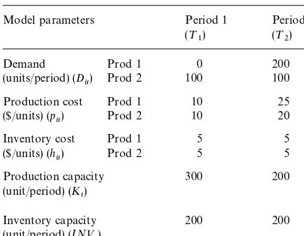
The objective of problem (8) is to determine the optimal production quantity and the inventory level in all theLplanning periods. This plan minim-izes the production and inventory holding costs and, at the same time, production and inventory capacities are respected. Problem (8) can be ex-tended by considering several stages of the pro-duction, distinguishing regular and over time productions, incorporating subcontractors, etc. Special conditions, production requirements and initial inventory levels can be formulated with additional constraints as well. Such models are widely discussed in the literature (see for example [1,13,14]). In almost all cases, however, the solution is degenerate. The problems and traps of sensitivity analysis of this type of models will be illustrated with a small size model determined by the data of Table 7.
The production quantity of two products (P
1
and P
2) in two production periods (¹1 and ¹2)
should be determined. The demand for P
1is zero in
the "rst and 200 units in the second period. The
demand for P
2 is 100 units in both periods. The
production cost is the same ($10 per unit) for both products in¹
1, and$25 per unit for P1, and$20 per
unit for P
2in¹2. The inventory holding cost is the
same in all periods for all products ($5 per unit). There is the capacity to produce 300 units in the
"rst period, and 200 units in the second period. The
inventory can not exceed 200 units in any of the two periods.
model in the standard form is obtained:
min (10x
1,1#10x2,1#25x1,2#20x2,2#5I1,1#5I2,1#5I1,2#5I2,2)
subject to
x
1,1 x !I1,1 "0,
2,1x !I2,1 "100,
1,2 x #I1,1 !I1,2 "200,
2,2 #I2,1 !I2,2 "100,
x
1,1#x2,1 #s1 "300,
x
1,2#x2,2 #s2 "200,
I
1,1#I2,1 I #s3 "200,
1,2#I2,2 #s4"200,
(9)
x
1,1,x2,1,x1,2,x2,2,I1,1,I2,1,I1,2,I2,2*0.
Table 7
Data of the production planning model Model parameters Period 1
(¹ 1)
Period 2 (¹
2) Demand
(units/period) (D
it)
Prod 1 0 200
Prod 2 100 100
Production cost ($/units) (p
it)
Prod 1 10 25
Prod 2 10 20
Inventory cost ($/units) (h
it)
Prod 1 5 5
Prod 2 5 5
Production capacity (unit/period) (K
t)
300 200
Inventory capacity (unit/period) (IN< t)
200 200
This small size problem can be solved with any LP software, but the optimal solution can be found easily by simple reasoning as well.
The data show that there is a considerable di! er-ence between the production costs in¹
1and in¹2.
It would be cheaper to produce all the products in ¹
1. The products demanded in ¹1 are produced
"rst. If there is free capacity, products demanded in
¹
2can be produced in¹1as well. After producing
100 units of P
2, there is free production capacity,
therefore the production of P
1demanded in ¹2is
scheduled for¹
1as well. The planned 200 units of
P
1 and 100 units of P2 are exactly equal to the
production capacity of the"rst period. There is also enough inventory capacity to store the 200 units of P
1until the second period. Since there is no more
free production capacity, the second period de-mand of P
2can not be produced in¹1, although it
would be advantageous "nancially. The optimal solution therefore is the following:
x
1,1"200; x2,1"100; x1,2"0; x2,2"100;
I
1,1"200; I2,1"0; I1,2"0; I2,2"0;
s
1"0; s2"100; s3"0; s1"200.
There are six nonzero values and the rank of the matrix of problem (9) is 8. Therefore the solution is primal degenerate, and since there is no alternative optimum, the solution is not dual degenerate. In
this case Type I and Type II sensitivities are the relevant information.
Solving the model with the STORM computer program, the same solution is gained. Apart from the optimal values of the production quantities and inventory levels, several important questions can be asked. First we will try to answer these questions logically, then, we will see what answer is provided by the sensitivity analysis results of the STORM computer program. The RHS sensitivities at two optimal basis (B
B
2"M1, 2, 3, 4, 5, 10, 11, 12N) are given in Tables
8 and 9. The objective function coe$cient sensitivi-ties atB
1andB2are provided in Tables 10 and 11.
(1) A new customer wants to buy P
1 in the xrst
period. How much will be the marginal cost of this
extra production?
The production cost of P
1 in ¹1 is$10. If one
extra unit should be produced in¹
1, then the
pro-duction of another unit, which was originally produced in ¹
1, but demanded in ¹2, has to be
produced in ¹
2 because of production capacity
limitations. The shift of the production of this one unit from ¹
1 to ¹2will increase production cost
from$10 to$25, and at the same time eliminates the
$5 inventory cost. The total cost of the shift is therefore $10 for every unit (25!10!5). The result is the sum of the production cost of the new product ($10) and the cost of shift ($10), which yields a $20 increase of the objective function for every unit of new P
1produced for¹1. There is 100
units free capacity in¹
2to reschedule P1.
There-fore, the $20 shadow price is valid as long as the new demand for P
1in the "rst period is less than
100 units.
When the program"nds the optimal solution at the basisB
1the sensitivity information is incorrect.
The $15 shadow price, shown in the "rst row of Table 8, is not the deduced value. The validity range shows that we are at a break point of the piecewise linear optimal value function.$15 is just a sub-di!erential, the true right and left derivatives might be di!erent from $15. When the optimal solution is found at the basisB
2then the sensitivity
information coincides with the deduced values ("rst row of Table 9).
(2) The demand forP
1 in the second period may
decrease or increase. How will this change the
opti-malvalue of the total cost?
Producing one unit less from P
1for¹2will result
in the savings of $10 production cost, and in the savings of $5 inventory holding cost because all P
(20!10!5). This is altogether$20 per unit. Since 100 units of P
1can be substituted by 100 units of
P
2, this$20 left side shadow price is true as long as
the demand decreases from 200 units to 100 units.
Table 8
RHS sensitivity of the production planning model at the optimal basisB
RHS sensitivity of the production planning model at the optimal basisB
CAP1 300 !10 200 300
y
When the demand for P
1increases by one unit in
¹
2, this extra quantity should be produced in
¹
2because in ¹1there is no free production and
inventory capacity. This will result in a$25 increase of the objective function for every unit (right side shadow price). Production can be increased up to 100 units as a consequence of the 100 units free production capacity in¹
2.
When the program "nds the optimum at the basisB
1then the left side shadow price and validity
range is provided (third row of Table 8). When the optimum is found at the basisB
2then the right side
(3) How much does the optimal total cost change if production capacity is increased by one unit in the
xrst period?
Since the 200 units of P
1is produced for¹2, it
should be kept in the warehouse. Inventory con-straints indicate that there is no more space to store, therefore the demand of P
2 in the second
period cannot be produced earlier, although," nan-cially it would be advantageous. Therefore, no mat-ter how much the production capacity is increased in ¹
1, it will not in#uence the objective function;
the shadow price is zero.
The zero shadow price cannot be found at any of the two basis, as the "fth rows of Tables 8 and 9 show.
(4) How much does the optimal total cost change if
the production capacity in the xrst period decreases
by one unit?
Since production capacity is fully utilized in¹
1,
the lost capacity will decrease the production of P
1.
If P
1is produced in ¹2production cost increases
by$15 (from$10 to$25) but inventory cost disap-pears ($5). The objective function therefore in-creases by$10 per unit. No more than 100 units of production can be shifted to¹
2because of capacity
limitations, therefore the$10 is valid when produc-tion capacity does not decrease below 200 units.
When the program "nds the optimum at the
B
1basis then the provided shadow price is wrong
("fth row of Table 8). The validity range indicates
that this is true just in the very near neighborhood of the current capacity, but from a practical point of view, this information is irrelevant. When the opti-mum is found at the B
2 basis then the answer is
right ("fth row of Table 9). The negative sign indi-cates that the decrease of capacity increases the objective function.
(5) How much does the optimal total cost change if
inventory capacity in thexrst period decreases by one
unit?
When the inventory capacity in ¹
1 decreases,
then production of P
1in¹1should be decreased,
because there is not enough inventory space to store those units of P
1which are produced for¹2.
Shifting the production of one unit of P
1to¹2will
increase the costs by$10 (25!10!5"10). No matter which basis is found, this information is not provided at any of the basis (seventh row of
Tables 8 and 9). The zero right side shadow price correctly indicates that there is no use increasing the inventory capacity because production capacity will impede any improvement of the production plan. There is no information, however, about the e!ect of the capacity decrease (left side shadow price).
(6) The production cost ofP
2in the second period
decreases. Will this require the change of the optimal
production plan?
At the current production cost it would be better to move the production of P
2to ¹1, but the
pro-duction capacity is fully utilized. When propro-duction cost of P
2decreases in¹2, the possible bene"t by
producing P
2in ¹1decreases as well. When
pro-duction cost drops to$15, the production cost in ¹
2will be equal to the production plus inventory
cost in¹
1, therefore shifting the production to¹1is
not advantageous any more. Since the production was not moved to¹
1because of the capacity
con-straints, this$15 is just a symbolic value. This value indicates that if we could change the plan it would be advantageous to do it as long as the production cost is higher than$15. But the correct answer to the question is that no matter how much the pro-duction cost of P
2in¹2decreases, the production
plan will stay optimal.
When the program"nds the optimal solution at the basisB
1then we may conclude that the
produc-tion plan should be changed when the cost de-creases below$15, because the fourth row of Table 10 indicates a$15 lower limit for the validity of the optimal production plan. When the B
2 basis is
found, then the right sensitivity information is given (fourth row of Table 11).
(7) The inventory holding cost of P
2 in the xrst
period increases. Will this change the optimal
pro-duction plan?
Since only the demand of P
2in¹1is scheduled
for production in¹
1, there is no inventory of P2in
the optimal production plan. It means, that no matter how much the inventory holding cost of P
2increases it will not in#uence the optimal plan. It
is true, however, that, reaching$10 has a symbolic importance. Above this level it will not be worth to move the production of all the P
2to¹1even if it
Table 10
The sensitivity of the objective function coe$cients of the pro-duction planning model at the optimum basisB
1
The sensitivity of the objective function coe$cients of the pro-duction planning model in the optimal basisB
2
production cost in¹
1plus the increased inventory
cost.
When the program"nds the optimal solution at basisB
1then we may conclude that the production
plan should be changed when the cost increases above$10, because the sixth row of Table 10 indi-cates a$10 upper limit for the validity of the opti-mal production plan. When basisB
2is found, then
the right sensitivity information is given (sixth row of Table 11).
(8) What is the bottleneck of this production
sys-tem, and how can the bottleneck capacity be
in-creased?
The bottleneck of this production system is con-stituted by both the production and inventory
capacities in ¹
1. Both should be increased if
de-mand in ¹
1 increases or production has to be
rescheduled from ¹
2 to ¹1. If both capacities
are increased by one unit, then one unit of produc-tion of P
2can be shifted from ¹2to¹1. This will
result in a$5 (20!10!5) decrease of the optimal total cost. This simultaneous increase of two RHS elements cannot be analyzed with the help of Tables 8 and 9.
In the following, some parameters of problem (9) will be modi"ed to get a more general case.Let the
production cost ofP
2in¹1be $5. As a consequence
of the decrease of production cost of P
2in¹1it is
even more advantages to produce all P
2in¹1. The
savings when the production of one unit of P
2 is
shifted from¹
2to¹1is$10 (20!5!5), which is
equal to the saving when one unit of P
1is shifted
from¹
2to¹1(25!5!10). Since in the original
problem 200 units of P
1were produced in advance,
and there is no production capacity in¹
1there are
alternative optima, because every unit of P
1
pro-duced in¹
1can be substituted by P2. Obviously,
then the substituted P
1should be produced in¹2. Let us relax the production capacity constraints as well, saying that there is capacity to produce 500
units in both periods. This is more than the total
demand for both products, therefore there is enough capacity to produce all P
1and P2in ¹1.
Obviously the existing inventory capacity does not allow to produce more units in ¹
1, although it
would be advantageous"nancially. The two alter-native optimal basis solutions in this case are the following:
Table 12
The three di!erent types of sensitivity ranges of the shadow price of the RHS of the inventory constraint of the"rst period (y
INV1"10)
Solution Basis Sensitivity range
of the basis
quence of the increase in the production capacities in each period. The value ofs
1is not zero any more.
Despite this change still there are seven nonzero values among the variables, and the rank of the matrix of problem (9) is 8. Therefore Optimum 1 is a primal degenerate optimal solution. This also means that more than one optimal basis belong to Optimum 1. In Optimum 2 the production of 100 units of P
1in¹1is substituted by 100 units of P2.
The 100 units substituted quantity of P
1has to be
produced in ¹
2. In this solution there are 8
non-zero variables. Therefore this optimum is not a pri-mal degenerate. Since the LP problem has two alternative optimal basis solutions, it is a dual de-generate.
Let us analyze the change in the capacity of the inventory (RHS of the inventory capacity con-straint) in¹
1. Since inventory capacity is the
limit-ing constraint, it does not allow the shiftlimit-ing of the production to ¹
1. When this 200 units capacity
increases by one unit, then one unit of P
1or P2can
be shifted to¹
1, and the gain is$10 in case of both
products. Therefore, the right side shadow price of the inventory capacity in¹
1is$10 per unit. In case
of Optimum 1, 100 units of P
1 and in case of
Optimum 2, 100 units of P
2can be shifted to¹1.
Therefore the capacity upper bound is 300 units (200#100). When the capacity of the inventory decreases, then there is no capacity to store the products produced in ¹
1 and used only in ¹2,
although it would be advantageous "nancially.
This "nancial advantage is $10 in case of each
product, which is the left side shadow price. In case of Optimum 1, 200 units of P
1can be shifted to¹2,
which results in a zero (200!200) lower bound of
the capacity decrease. In case of Optimum 2 there are two possibilities. When P
1is shifted from¹1to
¹
2there is no change of production plan, since 100
units of P
1are produced anyway in¹2. There is no
need to set up machines for new products, just more should be produced from P
1. In this case 100 units
of P
2can be shifted to ¹2which results in a 100
units lower bound for the validity range of the shadow price belonging to Optimum 2. Finally, 100 units of the P
2 can also be shifted to¹2but
this is a di!erent production plan, because ori-ginally machines were not set up for producing P
2Table 12 summarizes the provided sensitivityin¹2.
results for the RHS of inventory constraint in¹
1.
The modi"ed version of problem (9) is dual de-generate, therefore there are two optima. Opti-mum 1 is primal degenerate, and the sensitivity ranges found at the two optimal basis B
1 and
B
2 are listed in the third column of Table 12.
These are the left and right side sensitivity ranges. Since the left and right side shadow price is the same ($10 per unit) the sensitivity of Optimum 1 is the union of the left and right sensitivity ranges (column 4). Optimum 2 is not primal degenerate, therefore the sensitivity of the optimal basis is equal to the sensitivity of the optimal solution at
B
3, as it is indicated in column three and four.
Finally if this modi"ed problem is solved by an IPM solver we may get the following optimum:
IPM Optimum:
x
1,1"150; x2,1"150; x1,2"50; x2,2"50;
I
1,1"150; I2,1"50; I1,2"0; I2,2"0;
s
1"200; s2"400; s3"0; s1"200.
This is a strictly complementary optimal solution. Type II sensitivity in this case determines the range of a parameter within which the support sets of some appropriate optimal solutions are identical. The support set in this case represents a production plan in which every product is produced in every period and there is inventory of both products in
the "rst period. Because this is a strictly
com-plementary optimal solution, Type II and Type III sensitivities coincide.
In this small example it was possible to"nd out the right answers to the questions and check to what extent the sensitivity results at the di!erent optimal basis are correct. In complex problems, with several thousand constraints and variables, it is very di$cult to know how sensitivity analysis, provided by current programs, should be inter-preted (see for example [5,15]). Note that there is consistent mathematical theory to answer all the above questions correctly, typically one smaller LP has to be solved to get the answer to each question separately (see [8,12,16]). This is, however, not im-plemented yet in the existing commercial LP pack-ages, which is the shortcoming of the software and not the shortcoming of the theory. There is a lot of possibility to improve the sensitivity output of LP software.
f When these software are designed for managerial
use the sensitivity information concerning the
decision variables and/or the objective function
and not sensitivity information of the optimal basis should be presented. This requires some extra computation, but would certainly be a con-siderable help to users in the management area. Table 1 is an example of this type of sensitivity information.
f Bottleneck analysis is one of the most important
area in production management. When several resources constitute the bottleneck of the system
(the solution is degenerate) the information about the set of bottleneck resources and about the multiple change of the RHS elements is an essential information. Table 4, and the analysis of question 8 in Section 4 illustrates this problem. Note that this question can be treated by in-troducing a new variable that represents the simultaneous change of the RHS elements and sensitivity on this new variable is to be ob-tained. An easy and automatic performance of this analysis by the computer packages would be important.
f Finally the existence of alternative solutions
should be expressed more explicitly. The prob-lem of primal degeneracy is that, although the primal solution is unique, there are alternative dual optima. Turning this around, when a dual optimal solution is degenerate, then the primal optimum is not unique. In practical terms it means that several optimal production plans exist. For operations managers it would be useful to generate information about the multitude of the optimal plans, and decision on the selected one can be based on intangible criteria. Here we stress again, consistent mathematical theory exists for determining the dimension of the opti-mal sets when one uses IPMs. To provide this information would not increase the computa-tional cost at all.
5. Conclusions
irrelevant from the management decision point of view. Management wants to know either the sensi-tivity information concerning activities in an opti-mal solution (Type II sensitivity), or the sensitivity information concerning the objective function (Type III sensitivity).
The situation is a little di!erent in case of solvers based on the IPM, because these solvers provide strictly complementary solutions. These optimal solutions are not basis solutions. Therefore Type I sensitivity has no relevance. However using e$cient optimal basis identi"cation techniques, an optimal basis can be produced when needed. On the other hand, Type II and Type III information coincide in this case. But to distinguish among Type II and Type III sensitivity is important for decision mak-ing purposes, specially when a non-strictly com-plementary optimal solution is implemented.
Both the graphical solution of the small LP model and the logical solution of the production planning model have illustrated the existence of the three type of sensitivities.
Users should be careful when sensitivity results of an LP package are used for management decisions. Almost all practical size problems are degenerate, and the sensitivity information depends on the basis found by the computer program. Di!erent software may give di!erent results to the same model. Some-times the goodness of the sensitivity output can be checked by simple logic, but in most of the cases there is no direct way of evaluating the results.
Linear programming will probably stay one of the most popular operations research tool used in practice. The development of computer technology brought nearer this tool to inexperienced users. The interpretation of the sensitivity output of the cur-rently available software packages is di$cult and contains several traps because they provide only Type I sensitivity information. Software producers have a lot of possibility to help avoid the presented problems and to serve better the users in the man-agement area.
References
[1] L.A. Johnson, D.C. Montgomery, Operations research in production planning, in: Scheduling and Inventory Con-trol, Wiley, New York, 1974.
[2] J.R. Evans, N.R. Baker, Degeneracy and the (mis)inter-pretation of sensitivity analysis in linear programming, Decision Science 13 (1982) 348}354.
[3] D.C. Aucamp, D.I. Steinberg, The computation of shadow prices in linear programming, Journal of the Operational Research Society 33 (1982) 557}565.
[4] M. AkguKl, A note on shadow prices in linear program-ming, Journal of the Operational Research Society 35 (1984) 425}431.
[5] H.J. Greenberg, An analysis of degeneracy, Naval Re-search Logistics Quarterly 33 (1986) 635}655.
[6] T. Gal, Shadow prices and sensitivity analysis in linear programming under degeneracy, OR Spektrum 8 (1986) 59}71.
[7] D.S. Rubin, H.M. Wagner, Shadow prices: Tips and traps for managers and instructors, Interfaces 20 (1990) 150}157.
[8] B. Jansen, J.J. de Jong, C. Roos, T. Terlaky, Sensitivity analysis in linear programming: just be careful! European Journal of Operational Research 101 (1997) 15}28. [9] R.E. Wendell, The tolerance approach to sensitivity
analy-sis in linear programming, Management Science 31 (1985) 564}578.
[10] R.E. Wendell, Sensitivity analysis revisited and extended, Decision Sciences 23 (1992) 1127}1142.
[11] T. Gal, Postoptimal analysis, in: Parametric Programm-ing and Related Topics, McGraw-Hill, New York, 1986.
[12] C. Roos, T. Terlaky, J.-Ph. Vial, Theory and Algorithms for Linear Optimization}An Interior Point Approach, Wiley, Chichester, UK, 1997.
[13] S.C. Graves, A.H.G. Rinnooy Kan, P.H. Zipkin, Logistics of Production and Inventory, North-Holland, Amster-dam, 1993.
[14] S. Nahmias, Production and Operations Analysis, Irwin, Burr Ridge, 1993.
[15] A. Farkas, T. Koltai, A. Szendrovits, Linear programming optimization of a network for an aluminum plant: A case study, International Journal of Production Economics 32 (1993) 155}168.