An E
ffi
cient Bayesian Robust Principal Component Regression
Philippe Gagnona,∗, Myl`ene B´edarda, Alain Desgagn´eb
aD´epartement de math´ematiques et de statistique, Universit´e de Montr´eal, C.P. 6128, Succursale Centre-Ville,
Montr´eal, Qu´ebec, Canada, H3C 3J7
bD´epartement de math´ematiques, Universit´e du Qu´ebec `a Montr´eal, C.P. 8888, Succursale Centre-Ville, Montr´eal,
Qu´ebec, Canada, H3C 3P8
Abstract
Principal component regression is a linear regression model with principal components as regres-sors. This type of modelling is particularly useful for prediction in settings with high-dimensional covariates. Surprisingly, the existing literature treating of Bayesian approaches is relatively sparse. In this paper, we aim at filling some gaps through the following practical contribution: we intro-duce a Bayesian approach with detailed guidelines for a straightforward implementation. The approach features two characteristics that we believe are important. First, it effectively involves the relevant principal components in the prediction process. This is achieved in two steps. The first one is model selection; the second one is to average out the predictions obtained from the selected models according to model averaging mechanisms, allowing to account for model uncer-tainty. The model posterior probabilities are required for model selection and model averaging. For this purpose, we include a procedure leading to an efficient reversible jump algorithm. The second characteristic of our approach is whole robustness, meaning that the impact of outliers on inference gradually vanishes as they approach plus or minus infinity. The conclusions obtained are consequently consistent with the majority of observations (the bulk of the data).
Keywords: Dimension reduction, linear regression, outliers, principal component analysis, reversible jump algorithm, whole robustness.
2010 MSC: 62J05, 62F35
1. Introduction
Principal component regression (PCR) corresponds to the usual linear regression model in which the covariates arise from a principal component analysis (PCA) of some explanatory vari-ables. PCA is commonly used to reduce the dimensionality of data sets through two steps: first, the transformation of the “original” variables into principal components; second, the selection of the first d components, whered is smaller than the number of “original” variables. PCR is thus especially useful in situations where the number of explanatory variables is larger than the number
∗Corresponding author
Email addresses:[email protected](Philippe Gagnon),[email protected]
(Myl`ene B´edard),[email protected](Alain Desgagn´e)
of observations, or simply when one wishes to deal with smaller and therefore more stable mod-els. The price to pay is that we do not obtain the typical inference on the “original” explanatory variables (as the identification of which variables have a statistically significant relationship with the dependent variable). PCR is, as a result, mostly used for prediction. Still, it can be useful for elucidating underlying structure in these “original” explanatory variables, as explained and shown in the very interesting paper ofWest (2003). We focus on prediction in this paper, but we believe that our contributions can also be beneficial for elucidating underlying structure.
Traditionally, linear regression analysis assumes normality of the errors. We explain in Sec-tion 2.1 that this has the advantage that estimates are easily computed. A well-known problem however arises: inference may be contaminated by outliers. This problem is due to the slimness of the normal tails, which causes a shift in the posterior density to incorporate all data. It may find itself concentrated between the outliers and the bulk of the data, in an area that is not supported by any source of information. This translates into predictions that are not in line with either the nonoutliers or the outliers. FollowingBox and Tiao(1968) andWest(1984), we propose to model the errors in a different way, and more precisely, to replace the traditional normal assumption by an assumption that accommodates for the presence of outliers. This strategy is presented in Section2.2. We instead assume that the error term has a super heavy-tailed distribution that al-lows attaining whole robustness, as stated inGagnon et al.(2017b). Consequently, the predictions obtained reflect the behaviour of the bulk of the data.
Another challenge of PCR is the determination of which components to incorporate in the predictions. As a first step, we recommend to setd such that a predetermined percentage of the total variation is accounted for (provided that it is possible to do the estimation), as done inWest
(2003). In our analyses, we aim at reaching 90%. This step does not involve a study of the rela-tionship between the variable of interest and the components. West(2003) proposes, as a second step, to use a product of Student distributions centered at 0 as prior for the regression coefficients, seeking to attract towards 0 the coefficients that are not significantly far from this value. This supports the effort of dimension reduction. We believe this approach, although interesting, may contaminate the inference as the prior may act as “conflicting information”, in the sense that it may be in contradiction with the information carried by the data. The prior may have similar impact as outliers on the inference. We propose instead to identify the relevant components via model selection. More precisely, we introduce a random variableKrepresenting the model indicator and compute its posterior probabilities. Given that the components carrying significant information for prediction are usually the first ones, we considerdmodels, where ModelK =kis comprised of the firstkcomponents, k ∈ {1, . . . ,d}. This means that K also represents the number of components in a given model. This strategy aims at simplifying the computations. After having identified the relevant models, we propose to account for model uncertainty using model averaging (see, e.g.,
Raftery et al.(1997) andHoeting et al.(1999)). More precisely, we propose to identify models with posterior probabilities larger than 0.01, and to average over predictions arising from these models by weighting them according to the normalised probabilities. Model selection and model averaging allow to further reduce the dimensionality, while effectively considering the relevant components in predictions.
reversible jump algorithm. Indeed, it is a useful Markov chain Monte Carlo method introduced by
Green(1995) that allows switches between subspaces of differing dimensionality. It is thus a use-ful tool, not only for parameter estimation, but also for model selection; the method is described Section2.3. The implementation of such samplers requires the specification of some functions, and their efficiency relies heavily on their design (i.e. on how the functions are specified). In Section2.4, we provide a detailed procedure to implement an efficient reversible jump algorithm. The applicability and performance of our PCR approach is illustrated in Sections 3 and 4, containing respectively a simulation study and a real data analysis. The former is used to illustrate the performance of our approach under ideal conditions. The attained level of performance is used as a reference in the latter to establish that our method is suitable in real life situations.
2. Principal Component Regression
Consider that a PCA has been performed on p∈ {1,2, . . .}explanatory variables withn obser-vations each, from which the first d ∈ {1, . . . ,p} components are retained in order to be able to estimate the models (i.e.dis such thatn≥ d+1, see citegagnon2016regression for conditions that guarantee a proper posterior distribution). Let the associated design matrix be denoted by
X:=
x11 x12 · · · x1d
..
. ... . .. ... xn1 xn2 · · · xnd
,
where x11 = . . . = xn1 = 1, and xi j ∈ R for i = 1, . . . ,n and j = 2, . . . ,d. For simplicity,
we consider the vector (x11, . . . ,xn1)T = (1, . . . ,1)T as a component, but in fact, the principal components are the vectors (x12, . . . ,xn2)T, . . . ,(x1d, . . . ,xnd)T. These principal components are
such thatPn
i=1xi jxis = 0 for all j,s∈ {2, . . . ,d}with j , s(they are pairwise orthogonal vectors),
and (1/n)Pn
i=1xi j = 0 for all j ∈ {2, . . . ,d}(their mean is 0). They are ordered, as usual, by their
variability; the first one has the largest sample variance, the second one has the second largest sample variance, and so on.
The main goal is to study the relationship between a dependent variable, represented by the random variablesY1, . . . ,Yn ∈ R, and the covariates (the components) in order to predict values
for the dependent variable. We start from the premise that the following models are suitable:
Yi =(xKi )
TβK+ǫK
i , i=1, . . . ,n,
where K ∈ {1, . . . ,d} is the model indicator, which also represents the number of components included in the model (i.e. Model K = k is the model with the first k components), (xK
i ) T :=
(xi1, . . . ,xiK), ǫ1K, . . . , ǫnK ∈ R are n random variables that represent the error term of Model K,
and βK := (βK
1, . . . , βKK)T ∈ R K
is a vector comprised of K random variables that represent the regression coefficients of ModelK. The scale of the error term of ModelK is represented by the random variableσK > 0. Throughout the paper, the superscript indicates which model is used.
From this perspective of statistical modelling, we can achieve the main goal (study the rela-tionship between the dependent variable and the covariates for prediction purpose) through the identification of the relevant principal components (i.e. determination of the “best” models) and estimation of the parameters. Under the Bayesian paradigm, the model selection is performed consideringKas a random variable. In this paper, we choose to perform model selection and pa-rameter estimation simultaneously through the computation ofπ(k, σk,βk | y), the joint posterior distribution of (K, σK,βK) giveny:=(y
1, . . . ,yn).
A prior structure has to be determined to proceed with the computations. It is set to be fully non-informative, letting the data completely drive the inference. More precisely, we set the prior ofK, denotedπ(k), equal to 1/dfor allkin{1, . . . ,d}, the prior ofσK, denotedπ(σk), proportional
to 1/σk for σk > 0, and the conditional prior of βK
| K, denoted π(βk | k), proportional to 1 forβk ∈ Rk, which are the usual non-informative priors for these types of random variables. We
obviously assume the appropriate prior independence to obtain the following prior on (K, σK,βK):
π(k, σk,βk
) = π(k) × π(σk)
× π(βk | k) ∝ 1/σk for k
∈ {1, . . . ,d}, σk > 0, and βk
∈ Rk. It
might seem that the so-called Lindley paradox (Lindley (1957) and Jeffreys (1967)) may arise when using such prior structure. Casella et al. (2009) explain that this is due to the improper reference prior on the parameters π(σk,βk
| k) = c/σk, and propose a solution. The constant
c can indeed be arbitrarily fixed, and it can even be different for the different models. We are however consistant in our choices and use 1 for all models. We agree that this choice is arbitrary, but no approach is completely objective, including that ofCasella et al.(2009). We believe further theoretical investigations are needed to verify the validity of using such prior structure. That said, the model selection results presented in the numerical analyses are in line with those arising from the Bayesian information criterion (BIC, see Schwarz(1978)), which suggests that the paradox does not arise. Note that the approach proposed in this paper is still valid if informative priors are used, such as those inRaftery et al. (1997). If users are looking for simpler models, they can set the prior onK to penalise for the number of parameters in the same vein as the BIC. For instance, they can setπ(k)∝1/nk/2for allk∈ {1, . . . ,d}. A power different fromk/2 would result in a more (less) aggressive penalty if it is increased (decreased).
As is typically done in Bayesian linear regression, we assume that ǫK
1, . . . , ǫ
K
n andβ1K, . . . , β
K K
aren+ K conditionally independent random variables given (K, σK), with a conditional density forǫK
i given by
ǫiK |K, σK,βK =D ǫiK |K, σK ∼D(1/σK)f(ǫiK/σK), i= 1, . . . ,n. 2.1. First Situation: No Outliers
If one is sure that there is no outlier in the data, the most convenient way to model the errors is probably to assume their normality, i.e. f = N(0,1). Indeed, considering this assumption and using the structure of the principal components, estimates and model posterior probabilities have closed-form expressions, as indicated in Proposition1.
Proposition 1. Assuming that f = N(0,1), the posterior is given by
π(k, σk,βk |y)=π(k|y)π(σk |k,y)
k
Y
j=1
where
the sum over k of the expression on the right-hand side in (1).
Proof. See Section6.
Proposition1indicates that users can easily determine which Modelk∗has the highest posterior probability and estimate its parameters. Indeed, they can evaluateπ(k|y) (up to a constant) for all k∈ {1, . . . ,d}in order to find the maximum, and given Modelk∗, the parameters can be estimated using posterior means ˆβk1∗ = y¯ and ˆβkj∗ = Pn
i=1xi jyi/Pni=1x2i j for j = 2, . . . ,k∗ (if k∗ ≥ 2). In our
analyses, we use Bayesian model averaging (see Raftery et al. (1997)) to predict values for the dependent variable given sets of observations of the covariates. When normality is assumed, we can therefore useE[Yn+1 | y] = P
T. Note that, in this context of normality assumption, (σK)2
|K,yhas an inverse-gamma distribution with shape and scale parameters given by (n−k)/2 and (Pn
i=1y2i −n¯y
As explained in Section 1, an important drawback of the classical normal assumption on the error term is that outliers have a significant impact on the estimation. This issue is addressed in Section2.2.
2.2. Second Situation: Possible Presence of Outliers
the log-Pareto-tailed standard normal distribution, with parameters α > 1 andψ > 1. This is a distribution introduced byDesgagn´e(2015) that is expressed as
f(x)=
(2π)−1/2exp(−x2/2), if |x| ≤α,
(2π)−1/2exp(−α2/2)(α/|x|)(logα/log|x|)ψ, if |x|> α. (2)
It exactly matches the standard normal on the interval [−α, α], while having tails that behave like (1/|z|)(log|z|)−ψ (which is a log-Pareto behaviour). Assuming that the error term follows this
distribution and provided that there are at most⌊n/2−(d−1/2)⌋outliers (⌊·⌋is the floor function), Theorem 1 inGagnon et al.(2017b) indicates that the posterior distribution of (σK,βK) converges
towards the posterior of (σK,βK
) arising from the nonoutliers only, when the outliers approach plus or minus infinity, for any given model (i.e. for any givenK). Whole robustness is thus attained for any given model. Consider for instance a sample of sizen = 20 and that the first 7 components are retained for the analysis (i.e.d = 7). The convergence holds for any model if there is at most three outliers. The result ensures that, for any given model, any estimation of σK and βK based on posterior quantiles (e.g. using posterior medians and Bayesian credible intervals) is robust to outliers. Given that this result is valid for any given K, we conjecture that it is also valid for the whole joint posterior of (K, σK,βK); this is empirically verified in Sections3and4. In the analyses we setα= 1.96, which implies that ψ = 4.08, according to the procedure described in Section 4 of Desgagn´e (2015) (this procedure ensures that f is a continuous probability density function (PDF)). As explained in Gagnon et al. (2017b), setting α = 1.96 seems suitable for practical purposes.
2.3. Reversible Jump Algorithm
The price to pay for robustness is an increase in the complexity of the posterior. We conse-quently need a numerical approximation method for the computation of integrals with respect to this posterior. The method commonly used in contexts of model selection and parameter estima-tion within the Bayesian paradigm is the reversible jump algorithm, a Markov chain Monte Carlo method introduced byGreen(1995). The implementation of this sampler requires the specification of some functions, a step typically driven by the structure of the posterior. In the current context, we rely on Proposition1for specifying these functions. As illustrated inGagnon et al.(2017b), if there is no outlier, the posterior arising from an error term with density f as in (2) is similar to that arising from the normality assumption, for any given model. Furthermore, in presence of outliers, the posterior is similar to that arising from the normality assumption, but based on the nonoutliers only (i.e. excluding the outliers), again for any given model. Therefore, whether there are outliers or not, the posterior should have a structure similar to that expressed in Proposition 1. In other words, the posterior should reflect some kind of conditional independence between the regression coefficients, givenK andσK. We consider this feature to design the reversible jump algorithm. In particular, we borrow ideas fromGagnon et al. (2017a), in which an efficient reversible jump al-gorithm is built to sample from distributions reflecting a specific type of conditional independence (the sampler that we use is described in detail later in this section).
from a single output. One iteration of this sampler is essentially as follows: a type of movement is first randomly chosen, then a candidate for the next state of the Markov chain (that depends on the type of movement) is proposed. The candidate is accepted with a specific probability; if it is rejected, the chain remains at the same state. We consider three types of movements: first, updating of the parameters (for a given model); second, switching from ModelKto Model K+1 (this requires that a regression coefficient be added); third, switching from ModelKto ModelK−1 (this requires that a regression coefficient be withdrawn). The probability mass function (PMF) used to randomly select the type of movement is the following:
g(j) :=
τ, if j= 1,
(1−τ)/2, if j= 2,3, (3)
where 0 < τ < 1 is a constant. Therefore, at each iteration, an update of the parameters is attempted with probabilityτ, and a switch to either ModelK+1 or ModelK−1 is attempted with probability (1−τ)/2 in each case.
Updating the parameters of ModelKis achieved here by using a (K+1)-dimensional proposal distribution centered around the current value of the parameter (σK,βK
) and scaled according to ℓ/√K+1, where ℓ is a positive constant. We assume that each of the K + 1 candidates is generated independently from the others, according to the one-dimensional strictly positive PDF ϕi,i= 1, . . . ,K+1. Although the chosen PDFϕi usually is the normal density, using the PDF in
(2) induces larger candidate steps, and therefore, results in a better exploration of the state space. This claim has been empirically verified, and we thus rely on this updating strategy in the analyses in Sections3and 4. Note that one can easily simulate from (2) using the inverse transformation method.
A major issue with the design of the reversible jump algorithm is related to the fact that there may be a great difference between the “good” values for the parameters under ModelKand those under ModelK+1. As witnessed from the posterior density detailed in Proposition1, this should not be a concern in the case where there is no outlier. Furthermore, when the same data points are diagnosed as outliers for both ModelK and ModelK +1, this should not be a concern either, as explained previously. When observations are outliers with respect to ModelK+1 but not to Model Khowever, there will be a difference between the “good” values for the parameters of these models (because of the robustness provided by the super heavy-tailed distribution assumption). Therefore, when switching from ModelK to ModelK +1 for instance, the parameters that were already in Model K need to be moved to a position that is, combined with a candidate value for the new parameter, appropriate under Model K +1. Otherwise, this model switching will be less likely to be accepted, and if it is, it will possibly require some (maybe a lot of) iterations before the chain reaches the high probability area. This may result in inaccurate estimates. Existing research has focused on this issue (e.g.Brooks et al.(2003), Al-Awadhi et al. (2004), Hastie(2005), and
Karagiannis and Andrieu(2013)).
Our strategy is simple and easy to implement. First, add up the vector cK+1 to the current value of the parameters of Model K to end up in a suitable area under Model K + 1. Then, generate a valueuK+1for the new parameterβKK++11from a strictly positive PDFqK+1. The candidates
(σK,βK) are the current values of the parameters under ModelK. The rationale behind this is the
following. Suppose, for instance, thatβ1
1 (the intercept in Model 1) takes values around 0.5, but β21 (the intercept in Model 2) takes values around 1, while β22 takes values around 2 with a scale of 1. Setting c2 := (0,0.5)T andq
2 equal to the distribution given in (2) with location and scale parameters of 2 and 1, respectively, should result in a vector ((σ1,β1
)+c2,u2) that is in the high probability area under Model 2. Note that, in order not to obtain negative values forσK, we always set the first component of the vectorscito 0.
We now provide a pseudo-code for the reversible jump algorithm used to sample fromπ(k, σk,
βk | y) when assuming that f is given in (2). We thereafter explain how to specify the inputs required to implement it.
1. Initialisation: set (K, σK,βK)(0). Remark: the number in parentheses beside a vector (or a scalar) indicates the iteration index of the vector (or of the scalar). For instance, (K, σK,βK)
(m), wherem∈N, implies that the iteration index of any component in (K, σK,βK)(m) ism.
Iterationm+1.
2. Generateu∼ U(0,1).
3.(a) Ifu ≤ τ, attempt an update of the parameters. Generate a candidate wK(m) := (w 1, . . . , wK(m)+1), where w1 ∼ ϕ1(· | K(m), σK(m), ℓ), and wi ∼ ϕi(· | K(m), βKi−1(m), ℓ) for i = 2, . . . ,K(m)+1. Generateua ∼ U(0,1). If
ua ≤ 1∧
(1/w1)f(y|K(m),wK(m)) (1/σK(m))f(y|(K, σK,βK)(m))
!
,
where
f(y|k, σk,βk) :=
n
Y
i=1 1 σk f
yi−(xki)Tβk
σk
,
set (K, σK,βK)(m+1)= (K(m),wK(m)).
3.(b) Ifτ <u≤ τ+(1−τ)/2, attempt adding a parameter to switch from ModelK(m) to Model K(m)+1. GenerateuK(m)+1∼ qK(m)+1and generateua∼ U(0,1). If
ua ≤ 1∧
π(K(m)+1)f(y|K(m)+1,(σK,βK)(m)+cK(m)+1,uK(m)+1) π(K(m))f(y|(K, σK,βK)(m))q
K(m)+1(uK(m)+1)
!
,
set (K, σK,βK)(m+1)= (K(m)+1,(σK,βK)(m)+cK(m)+1,uK(m)+1).
3.(c) Ifu> τ+(1−τ)/2, attempt withdrawing the last parameter to switch from ModelK(m) to ModelK(m)−1. Generateua ∼ U(0,1). If
ua ≤
1∧
π(K(m)−1)f(y|K(m)−1,(σK,βK−)(m)−cK(m))q
K(m)(βKK(m)) π(K(m))f(y|(K, σK,βK)(m))
,
set (K, σK,βK)(m+1)= (K(m)
−1,(σK,βK−)(m)−cK(m)), where (σK,βK−)(m) is (σK,βK)(m)
without the last component (more precisely, (σK,βK−)(m) :=(σK, βK
1, . . . , β
K
5. Go to Step 2.
It is easily verified that the resulting stochastic process {(K, σK,βK)(m),m
∈ N} is aπ(k, σk,
βk |y)-irreducible and aperiodic Markov chain. Furthermore, it satisfies the reversibility condition with respect to the posterior, as stated in the following proposition. Therefore, it is an ergodic Markov chain, which guarantees that the Law of Large Numbers holds.
Proposition 2. Consider the reversible jump algorithm described above. The Markov chain
{(K, σKβK)(m),m ∈ N} satisfies the reversibility condition with respect to the posterior π(k, σk,
βk |y)arising from the assumption that f is given in (2).
Proof. See Section6.
2.4. Optimal Implementation
In order to implement the reversible jump algorithm described above, we have to specify the PDFsqi, the constantsτandℓ, and the vectorsci. In the following paragraphs, we explain how we
achieve this task.
InGagnon et al.(2017a), a simple structure for the posterior is considered in order to obtain theoretical results that lead to an optimal design of the reversible jump algorithm. The structure is the following. The parameters are conditionally independent and identically distributed for any given model. The model indicator K indicates the number of parameters that are added to the simplest model (the one with the fewest parameters). Finally, when switching from Model K to Model K+ 1 (i.e. when adding a parameter), the distributions of the parameters that were in Model K do not change. The authors find asymptotically optimal (as the number of parameters approaches infinity) values forτandℓ. They conjecture that their results are valid (to some extent) when the parameters are conditionally independent, but not identically distributed, for any given model. They also provide guidelines to suitably design the PDFs qi. Their setting is somewhat
similar to ours, because, as explained above, the posterior should reflect some kind of conditional independence between the regression coefficients, given K andσK. Also, when switching from
ModelKto ModelK+1, if there is no outlier or if the same data points are diagnosed as outliers for both models, there should not be a great difference between the “good” values for the parameters under ModelKand those under ModelK+1. We therefore use their results to design the reversible jump algorithm (at least as a starting point).
In the setting ofGagnon et al.(2017a), the asymptotically optimal value for τdepends on the PDFs qi. But for moderate values of d, selecting any value between 0.2 and 0.6 seems almost
optimal. We recommend to setτ= 0.6 ifd is rather small (because there are not so many models to visit), as in our analyses in Sections3 and 4. Selecting larger values for τleaves more time between model switchings for the chain to explore the state space of the parameters. We ran several reversible jump algorithms with different values for τ to verify if 0.6 actually is a good choice. The optimal values are close to 0.6 for the data sets analysed in Sections3and4.
If the parameters (σK,βK
in which there has been an attempt at updating the parameters. If the parameters are nearly in-dependent but not identically distributed, the asymptotically optimal value may correspond to an acceptance rate smaller than 0.234, as explained inB´edard(2007). If in addition σK has a great impact on the distribution of βK, the asymptotically optimal value may correspond to a further reduced acceptance rate, as explained in B´edard(2015). Considering this, combined to the fact thatd can be rather small, we recommend to perform trial runs to identify the optimal value for ℓ. We use the 0.234 rule to initiate the process. In our analyses in Sections3and4, the optimal values forℓcorrespond to acceptance rates relatively close to 0.234.
We propose to specify the PDFsqi and the vectors ci through trial runs too. Specifying these
functions and vectors requires information about the location of all regression coefficients for all models and about the scaling ofβK
K for Model K, K ≥ 2. In order to gather this information and
to identify the optimal value forℓ, we propose a naive but simple strategy for the trial runs that can be executed automatically: run a random walk Metropolis (RWM) algorithm for each model. The RWM algorithm is the reversible jump algorithm described above in which τ = 1 (it is an algorithm in which only updates of the parameters are proposed). Here is the procedure that we recommend for the trial runs:
For eachk∈ {1, . . . ,d}:
1. Tune the value of ℓ so that the acceptance rate of candidates wk is approximately 0.234.
Record the corresponding valueℓk.
2. Select a sequence of values forℓ aroundℓk: (ℓ
1, . . . , ℓj0 := ℓ
k, . . . , ℓ
L), where Lis a positive
integer.
3. For each ℓj: run a RWM algorithm with: (σk(0))2 ∼ Inv-Γwith shape and scale parameters
given by (n−k)/2 and (Pn
i=1y2i −n¯y
2
−1(k ≥ 2)Pk j=2(
Pn
i=1xi jyi)2/Pni=1x2i j)/2, respectively,
βk
1(0) ∼ N(¯y,(σ
k(0))2/n), andβk
j(0)∼ N(
Pn
i=1xi jyi/Pni=1x2i j,(σk(0))2/
Pn
i=1x2i j), j= 2, . . . ,k
(ifk≥ 2).
4. For each ℓj: estimate the location of each of the parameters βki using the median (that we
denotemki,j) of{βki(m),m∈ {B+1, . . . ,T}}, fori= 1, . . . ,k, whereBis the length of the burn-in period andT is the number of iterations. If k ≥ 2, estimate the scaling of βkk using the interquartile range (IQR) divided by 1.349 (that we denotesk
k,j) of{β k
k(m),m∈ {B+1, . . . ,T}}
(this is robust measure of the scaling). Measure the efficiency of the algorithm with respect toℓj using the integrated autocorrelation time (IAT) of{σk(m),m ∈ {B+1, . . . ,T}}. Recall
that all parameters move at the same time when there is an update of the parameters, which indicates that this efficiency measure is appropriate. Record the valueℓk
opt corresponding to the smallest IAT.
5. Change the sequence of values for ℓ if the smallest IAT corresponds to the lower or upper bound of the current range.
6. Compute the average of{mk
i,1, . . . ,m
k
i,L}(that we denotem
k
i) fori=1, . . . ,k, and the average
of{skk,1, . . . ,skk,L}(that we denoteskk).
that the intercept estimate is the same for all models and that it is ¯y), and mjj = mjj+1 = . . . =
md j =
Pn
i=1xi jyi/Pin=1xi j2 (which indicates that the jth regression coefficient estimate is the same
for all models and that it isPn
i=1xi jyi/Pin=1x2i j) for j = 2, . . . ,d. If it is the case, it indicates that
there should not be any outliers because the estimates are the same as when assuming normality (see Proposition 1). Consequently, users may assume normality of the errors and proceed as in Section2.1for the computation of the predictions. Otherwise, setqjequal to the distribution given
in (2) with location and scale parameters given by mjj and sjj, respectively, for j = 2, . . . ,d. Set cj =(0,m1j −m1j−1, . . . ,mjj−1−mjj−−11)T, for j=2, . . . ,d. Setℓequal to the median of{ℓ1opt, . . . , ℓdopt}. The only remaining inputs required to implement the reversible jump algorithm are initial values for the model indicator and the parameters. We recommend to generateK(0)∼ U{1, . . . ,d}, (σK(0))2 ∼ Inv-Γ with shape and scale parameters given by (n − K(0))/2 and (Pn
i=1y2i − n¯y
2
−
1(K(0) ≥ 2)PK(0)
j=2(
Pn
i=1xi jyi)2/Pni=1x2i j)/2, respectively, β K
1(0) ∼ N(m
K(0) 1 ,(s
K(0) 1 )
2), and βK j(0) ∼ N(mKj(0),(sKj(0))2), j = 2, . . . ,K(0) (if K(0)
≥ 2). In the analyses in Sections 3 and 4, we use sequences of lengthL=10 forℓ,T =100,000 iterations and a burn-in period of lengthB=10,000 for the trial runs. When running the reversible jump, we use 1,000,000 iterations and a burn-in period of length 100,000.
3. Simulation Study
Through this simulation study, we empirically verify the conjecture stated in Section2.2about the convergence of the posterior of (K, σK,βK) towards that arising from the nonoutliers only when the outliers approach plus or minus infinity. A framework that includes the presence of large outliers is thus set up. This can be considered as ideal conditions for the application of our method (given that this simulates the limiting situation). This nevertheless also allows to illustrate the performance of our approach under these conditions (recall that in the next section, its performance is evaluated when applied to a real data set). To help evaluate the performance, we compare the results with those arising from the normality assumption. The impact of model selection and model averaging is not analysed. We believe that the beneficial effect of these statistical techniques is well understood, contrary to that of using super heavy-tailed distributions in linear regression analyses. Indeed, this strategy has been recently introduced inDesgagn´e and Gagnon(2017), in which the special case of simple linear regressions through the origin is considered. Then, its validity when applied the usual linear regression model was verified inGagnon et al.(2017b). It is the first time that this strategy is considered in a context of model selection.
We begin by generatingn = 20 observations from explanatory variables. We shall work with 24 such variables which, by construction, are expected to be represented by 4 principal com-ponents. We define the vectors u1 := (1, . . . ,20)T, u2 := (02,12, . . . ,192)T, u3 := (log(1), . . . , log(20))T, and u
4 := (exp(1), . . . ,exp(20))T. From these vectors, four orthogonal, centered, and standardised vectors e1, . . . ,e4 are obtained through the Gram-Schmidt method. The vec-torse1, . . . ,e4 represent the observations from the first four explanatory variables. The remaining 20 explanatory variables are obtained from e1, . . . ,e4, introducing correlation between the ex-planatory variables. More precisely, for each of the vectors ei, we generate five vectors from a
the elements on the diagonal is arbitrarily set to 0.12.
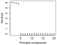
From these variables, we first generate observations from the dependent variable using the lin-ear regression model with a normal error term. The intercept and the second regression coefficient are arbitrarily set to 10 and 1, respectively, and each of the following regression coefficients are equal to minus the half of the previous one (therefore,−1/2, 1/4, and so on). The scale parameter of the error term is arbitrarily set to 1. We now perform the statistical analysis of the resulting data set. We shall then add a large outlier to evaluate the impact on the estimation (and therefore, on the predictions) under both the normality and the super heavy-tailed distribution assumptions. We apply the PCA on the initial data set and selectdupon examining the variation explained by each of the principal components (see Figure1and Table1).
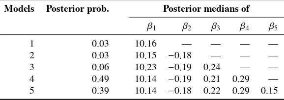
As expected, everything suggests that we should retain 4 principal components, and therefore, selectd = 5. We now compute the posterior probabilities of the models and the parameter esti-mates. The results under the super heavy-tailed distribution assumption are presented in Table2.
● ● ●●
● ● ● ● ● ● ● ● ● ● ● ● ● ● ● ●
5 10 15 20
0
1
2
3
4
5
6
Principal components
V
ar
iance
Figure 1:Sample variance for each of the principal components
Princ. comp. Cum. expl. var. (in %)
1 25.48
2 50.53
3 75.29
4 99.47
Table 1: Cumulative explained variations for the four first principal components
We notice that the parameter estimates do not vary significantly from one model to another. As explained in Section2.2, this is expected when there is no outlier or when the same data points are diagnosed as outliers for all models. The results under normality assumption are essentially the same, which suggests the absence of outliers. In particular, the posterior probabilities of Models 1 to 5 are 0.02, 0.02, 0.04, 0.49, and 0.42, respectively. The estimates of the first to the fifth regres-sion coefficients are 10.14, −0.18, 0.21, 0.28, and 0.15, respectively. Therefore, predictions shall be essentially the same under both assumptions, provided that we use ˆyn+1 = Pkπ(k |y)(xkn+1)
Tβˆk
in both cases, along with posterior medians under the super heavy-tailed distribution assumption. We now add an outlier to the data set. In order to preserve the properties on the columns in the design matrix X containing the principal components, we set xd
21 = (1,0, . . . ,0)
T, ensuring
that the conclusions of Proposition1still hold. Indeed, the vectors comprised of the observations from the covariates are still pairwise orthogonal and their mean is still 0. This prevents us from doing another PCA, and therefore, facilitates the comparison of results. We sety21 = 30, a large outlier compared with the trend emerging from the bulk of the data (this can correspond to the estimated intercept from the original data set for most models, i.e. ˆβK
1 = 10.14). With or without the outlier, the estimates forβKi ,i=2, . . . ,5,under normality do not vary; recall that they are given by ˆβK
i =
Pn
i=1xi jyi/Pni=1x2i j,i=2, . . . ,5. The estimates forβ K
1 andσ
K are however different: while
ˆ βK
outlier thus mainly translates into higher probabilities on large scale parameter values for the error term. This is due to the position of the outlier (the impact of an outlier with a different position is shown in Section4). Its impact is however not only on the marginal posterior distributions ofσK andβK
1. It propagates through the whole joint posterior of K, σ
K andβK, increasing the posterior
scaling of the entire vectorβK and modifying the posterior probabilities of the models. The latter are 0.12, 0.14, 0.18, 0.25 and 0.32, respectively for Models 1 to 5.
The results under the super heavy-tailed distribution assumption are now presented in Table3. Whole robustness seems attained. Indeed, the posterior probabilities of the models and the pa-rameter estimates are essentially the same as those based on the original data set. As a result, predictions made under the super heavy-tailed distribution assumption reflect the behaviour of the bulk of the data, contrary to those made under normality. In other words, new observations from the dependent variable in line with the bulk of the data are more accurately predicted under the robust approach.
4. Real Data Analysis: Prediction of Returns for the S&P 500
In Section 3, we showed that our strategy allows to obtain adequate inference in presence of large outliers, corresponding to an ideal condition for the application of our method. In this section, we show how our strategy performs when applied to a real data set containing outliers. Again, the results obtained from our method are compared with those arising from the normality assumption.
Models Posterior prob. Posterior medians of
β1 β2 β3 β4 β5
1 0.02 10.15 — — — —
2 0.02 10.14 −0.19 — — —
3 0.06 10.23 −0.20 0.25 — —
4 0.49 10.14 −0.19 0.21 0.28 — 5 0.41 10.14 −0.18 0.22 0.28 0.15
Table 2:Posterior probabilities of models and parameter estimates under the super heavy-tailed distribution assumption based on the data set without outliers
Models Posterior prob. Posterior medians of
β1 β2 β3 β4 β5
1 0.03 10.16 — — — —
2 0.03 10.15 −0.18 — — —
3 0.06 10.23 −0.19 0.24 — —
4 0.49 10.14 −0.19 0.21 0.29 — 5 0.39 10.14 −0.18 0.22 0.29 0.15
The context is the following: we model the January 2011 daily returns of the S&P 500 by exploiting their potential linear relationship with some financial assets and indicators, aiming at predicting the February 2011 daily returns of this stock index. The detailed list of explanatory variables is provided in Section7. There are 18 explanatory variables in total, and obviously, their observations on dayiare used to predict the return of the S&P 500 on dayi+1. For each of the explanatory variables and for the dependent variable, there aren = 19 observations that can be used to estimate the models, and the linear regression model with all explanatory variables has 20 parameters (18 regression coefficients for the variables, the intercept, and the scale parameter). The PCA should be a beneficial procedure given that financial assets and indicators are likely to carry redundant information.
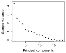
As in Section 3, we start by selectingd. We decide to retain 10 principal components which account for approximately 92% of the total variation (see Figure2and Table4), and therefore, to setd =11.
●
● ●
●
● ● ● ●
● ●● ● ●
● ● ● ● ●
5 10 15
0
1
2
3
4
Principal components
Sample v
ar
iance
Figure 2:Sample variance for each of the principal components
Princ. comp. Cum. expl. var. (in %)
8 84.87
9 88.80
10 92.45
11 95.51
Table 4: Cumulative explained variations for the first eighth to eleventh components
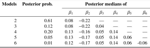
We now present the results under the super heavy-tailed distribution assumption in Table 5. The posterior probabilities of models other than 2 to 6 are all less than 0.01. We notice from Table 5 that outliers seem present with respect to either Models 2 and 3 or Models 4, 5 and 6 (because parameter estimates are significantly different). To help us in this outlier investigation, we now present the results under the normality assumption. The probabilities of Models 2 to 6 are 0.92, 0.07, 0.01, 0.00, and 0.00 (to two decimal places), respectively, and the estimates of the first to sixth regression coefficients are 0.06,−0.23, 0.03, 0.08, 0.06, and −0.09, respectively. This suggests that there are outliers with respect to Models 4, 5, and 6 (because the parameter estimates under the normality assumption are different from those under the super heavy-tailed distribution assumption for these models). It is noteworthy that Model 4 is an unlikely model under the normality assumption, but a relatively likely model under the super heavy-tailed assumption. This leads, along with the discrepancies in the parameter estimates, to different predictions. In particular, the mean absolute deviation between the predicted and actual returns in percentage for February 2011 is 0.62% under the normality assumption, whereas it is 0.57% under the super heavy-tailed distribution assumption. Under both assumptions, we use the same expression to predict, i.e. ˆyn+1 = Pkπ(k | y)(xkn+1)
Tβˆk, but the estimates are posterior medians for the super
normality and the super heavy-tailed assumptions.
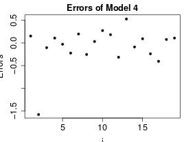
We now identify the outliers and redo the statistical analysis excluding these observations to evaluate their impact. For the identification step, we compute the errors, i.e. yi − (xki)Tβˆ
k
,i =
1, . . . ,19, of Model 4 (the most probable model among those for which there are outliers) under the super heavy-tailed assumption (see Figure 3). Note that the computation of these errors is based on the data used to estimate the models, i.e. the January 2011 daily returns.
●
● ●
● ●
● ●
● ●
● ●
● ●
● ●
● ●
● ●
5 10 15
−1.5
−0.5
0.0
0.5
Errors of Model 4
i
Errors
Figure 3:Errors of Model 4 under the super heavy-tailed assumption computed using posterior medians
The second observation seems to be not in line with the trend emerging from the bulk of the data. This is also true under Models 5 and 6. The results excluding this observation under the super heavy-tailed distribution assumption are presented in Table6. Again, the probabilities of models other than 2 to 6 are all less than 0.01. The results under the normality assumption are now essentially the same. Note that the conclusions of Proposition1 do not hold any more. Indeed, without the second observation, the properties on the columns in the design matrix are not preserved. The reversible jump algorithm has therefore been used, and the strategy explained in Section2.2to design it has been applied.
The second observation has a significant impact on the posterior distribution under the nor-mality assumption. The robust alternative is able to limit the impact (as can be seen by comparing the results in Table 5with those in Table 6). In fact, this example illustrates another feature of our method. It has the ability of reflecting the level of uncertainty about the fact that an obser-vation really is an outlier or not. This phenomenon was discussed in Gagnon et al.(2017b). In this example, the method seems to diagnose the second observation as an outlier (which explains why it limits its impact), but not as a “clear” outlier, as it does in Section3with the twenty-first observation. It is a question of whether or not the observation is far enough from the bulk of the data, and more precisely, far enough from the probable hyperplanes for the bulk of the data. Note that the differences between the predictions made under the two different assumptions, based on the original data set, are due to the presence of second observation. Indeed, without this observa-tion they are the same. In particular, the mean absolute deviaobserva-tion between the predicted and actual returns in percentage is now 0.50% (it is 0.57% for the robust approach with the outlier), and the number of correct predictions of whether the S&P 500 will go up or down is 12 (it also 12 for the robust approach with the outlier).
5. Conclusion and Further Remarks
Models Posterior prob. Posterior medians of
β1 β2 β3 β4 β5 β6
2 0.61 0.08 −0.22 — — — —
3 0.12 0.08 −0.22 0.04 — — —
4 0.20 0.13 −0.16 0.05 0.14 — —
5 0.05 0.13 −0.17 0.05 0.14 0.06 — 6 0.01 0.12 −0.17 0.05 0.14 0.06 -0.06
Table 5:Posterior probabilities of models and parameter estimates under the super heavy-tailed distribution assumption based on the returns in %
Models Posterior prob. Posterior medians of
β1 β2 β3 β4 β5 β6
2 0.16 0.13 −0.17 — — — —
3 0.04 0.13 −0.16 0.05 — — —
4 0.61 0.15 −0.15 0.06 0.16 — —
5 0.16 0.15 −0.15 0.06 0.16 0.06 — 6 0.03 0.15 −0.15 0.06 0.16 0.06 -0.04
Table 6:Posterior probabilities of models and parameter estimates under the super heavy-tailed distribution assumption based on the returns in %, without the second observation
(and how to involve them); second, how to limit the impact of outliers so that inferences are not contaminated. All the required guidelines for a straightforward implementation of our method have been provided. In particular, a detailed procedure to implement an efficient reversible jump algorithm has been included, allowing to obtain the required model posterior probabilities and parameter estimates. The relevance of our approach has been shown via a simulation study and a real data analysis in Sections3and4, respectively.
The method used to reduce dimensionality in our paper is the traditional PCA. Recall that this method transforms the “original” explanatory variables into principal components. This trans-formation is based on the sample correlation matrix of the observations from the explanatory variables. This process can be contaminated if there are outliers among these observations. The approach to attain robustness presented in this paper can thus be viewed as a first step towards fully robust PCR. Further research is therefore needed. We believe it would be particularly useful to develop a robust procedure to reduce dimensionality that also induces sparsity to deal with the case of interestp≫ n.
References
References
Al-Awadhi, F., Hurn, M., Jennison, C., 2004. Improving the acceptance rate of reversible jump MCMC proposals. Statist. Probab. Lett. 69 (2), 189–198.
B´edard, M., 2015. On the optimal scaling problem of Metropolis algorithms for hierarchical target distributions, preprint.
Box, G. E. P., Tiao, G. C., 1968. A Bayesian approach to some outlier problems. Biometrika 55 (1), 119–129. Brooks, S. P., Giudici, P., Roberts, G. O., 2003. Efficient construction of reversible jump Markov chain Monte Carlo
proposal distributions. J. R. Stat. Soc. Ser. B. Stat. Methodol. 65 (1), 3–39.
Casella, G., Gir`on, F. J., Mart´ınez, M. L., Moreno, E., 2009. Consistency of Bayesian procedures for variable selection. Ann. Statist. 37 (3), 1207–1228.
Desgagn´e, A., 2015. Robustness to outliers in location–scale parameter model using log-regularly varying distribu-tions. Ann. Statist. 43 (4), 1568–1595.
Desgagn´e, A., Gagnon, P., 2017. Bayesian robustness to outliers in linear regression and ratio estimation, submitted for publication.
Gagnon, P., B´edard, M., Desgagn´e, A., 2017a. Weak convergence and optimisation of the reversible jump algorithm, submitted for publication.
Gagnon, P., Desgagn´e, A., B´edard, M., 2017b. Bayesian robustness to outliers in linear regression, submitted for publication.
Green, P. J., 1995. Reversible jump Markov chain Monte Carlo computation and Bayesian model determination. Biometrika 82 (4), 711–732.
Hastie, D., 2005. Towards automatic reversible jump markov chain monte carlo. Ph.D. thesis, University of Bristol. Hoeting, J. A., Madigan, D., Raftery, A. E., Volinsky, C. T., 1999. Bayesian model averaging: A tutorial. Statist. Sci.,
382–401.
Jeffreys, H., 1967. Theory of Probability. Oxford Univ. Press, London.
Karagiannis, G., Andrieu, C., 2013. Annealed importance sampling reversible jump MCMC algorithms. J. Comp. Graph. Stat. 22 (3), 623–648.
Lindley, D. V., 1957. A statistical paradox. Biometrika 44 (1), 187–192.
Raftery, A. E., Madigan, D., Hoeting, J. A., 1997. Bayesian model averaging for linear regression models. J. Amer. Statist. Assoc. 92 (437), 179–191.
Schwarz, G., 1978. Estimating the dimension of a model. Ann. Statist. 6 (2), 461–464.
West, M., 1984. Outlier models and prior distributions in Bayesian linear regression. J. R. Stat. Soc. Ser. B. Stat. Methodol. 46 (3), 431–439.
West, M., 2003. Bayesian factor regression models in the “large p, small n” paradigm. In: Bayesian Statistics 7. Oxford Univ. Press, London, pp. 723–732.
6. Proofs
Proof of Proposition1. The proof is essentially a computation using that f = N(0,1) and the structure of the principal components. First,
π(k,(σk,βk)|y)∝ f(y|k,(σk,βk))π(k)π(σk)π(βk |k)∝ f(y|k,(σk,βk))(1/σk)π(k).
The likelihood function for a given model is
f(y|k,(σk,βk))=
n
Y
i=1 1
σk√2πexp
(
− 1
2(σk)2(yi−(x
k i)
T
βk)2
)
= 1
(σk)n(2π)n/2exp
− 1
2(σk)2
n
X
i=1
(yi−(xki) Tβk)2
We now analyse the sum in the exponential:
Putting this together leads to:
π(k,(σk,βk)|y)∝ π(k) 1
Proof of Proposition2. As explained inGreen(1995), it suffices to separately verify that the prob-ability to go from a setAto a set Bis equal to the probability to go fromBtoAwhen updating the parameters and when switching models, for accepted movements and for all appropriateA,B.
When updating the parameters, the probability to go from a setAto a setBis given by
Z
and, using Fubini’s theorem, this probability yields
Z
This last probability is equal to
Z
which is the probability to switch from Modelk+1, where the parameters are in the setA′×B, to Modelk, where the parameters are in the setA.
Therefore, the Markov chain{(K(m),(σK(m),βK(m))(m)),m
∈ N}satisfies the reversibility
7. Appendix
Name Ticker symbol
Artis Real Estate Investment Trust AX-UN.TO
Asanko Gold Inc. AKG.TO
Bonterra Energy Corp. BNE.TO
Canadian Imperial Bank Of Commerce CM.TO
CI Financial Corp. CIX.TO
Celestica Inc. Subordinate Voting Shares CLS.TO
DHX Media Ltd. DHX-B.TO
Dominion Diamond Corporation DDC.TO
Gildan Activewear Inc. GIL.TO
Husky Energy Inc. HSE.TO
iPath Bloomberg Sugar Subindex SGG
iShares MSCI Japan EWJ
iShares 20+Year Treasury Bond TLT
Laurentian Bank of Canada LB.TO
Parkland Fuel Corporation PKI.TO
United States Oil Fund LP USO
Vermilion Energy Inc. VET.TO
Volume of the S&P 500 N/A