M820
The Calculus of Variations
and Advanced Calculus
Contents
1 Preliminary Analysis 9
1.1 Introduction . . . 9
1.2 Notation and preliminary remarks . . . 12
1.2.1 The Order notation . . . 14
1.3 Functions of a real variable . . . 16
1.3.1 Introduction . . . 16
1.3.2 Continuity and Limits . . . 16
1.3.3 Monotonic functions and inverse functions . . . 19
1.3.4 The derivative . . . 19
1.3.5 Mean Value Theorems . . . 24
1.3.6 Partial Derivatives . . . 26
1.3.7 Implicit functions . . . 30
1.3.8 Taylor series for one variable . . . 33
1.3.9 Taylor series for several variables . . . 38
1.3.10 L’Hospital’s rule . . . 40
1.3.11 Integration . . . 41
1.4 Miscellaneous exercises . . . 48
1.5 Solutions for chapter 1 . . . 53
2 The Calculus of Variations 79 2.1 Introduction . . . 79
2.2 The shortest distance between two points in a plane . . . 79
2.2.1 The stationary distance . . . 80
2.2.2 The shortest path: local and global minima . . . 82
2.2.3 Gravitational Lensing . . . 84
2.3 Two generalisations . . . 85
2.3.1 Functionals depending only upony′(x) . . . . 85
2.3.2 Functionals depending uponxandy′(x) . . . . 87
2.4 Notation . . . 88
2.5 Examples of functionals . . . 90
2.5.1 The brachistochrone . . . 90
2.5.2 Minimal surface of revolution . . . 92
2.5.3 The minimum resistance problem . . . 92
2.5.4 A problem in navigation . . . 96
2.5.5 The isoperimetric problem . . . 96
2.5.6 The catenary . . . 97
2.5.7 Fermat’s principle . . . 98
2.5.8 Coordinate free formulation of Newton’s equations . . . 100
2.6 Miscellaneous exercises . . . 102
2.7 Solutions for chapter 2 . . . 106
3 The Euler-Lagrange equation 117 3.1 Introduction . . . 117
3.2 Preliminary remarks . . . 118
3.2.1 Relation to differential calculus . . . 118
3.2.2 Differentiation of a functional . . . 119
3.3 The fundamental lemma . . . 123
3.4 The Euler-Lagrange equations . . . 124
3.4.1 The first-integral . . . 126
3.5 Theorems of Bernstein and du Bois-Reymond . . . 130
3.5.1 Bernstein’s theorem . . . 131
3.5.2 The contrast between initial and boundary value problems . . . . 133
3.6 Strong and Weak variations . . . 134
3.7 Miscellaneous exercises . . . 137
3.8 Solutions for chapter 3 . . . 142
4 Applications of the Euler-Lagrange equation 161 4.1 Introduction . . . 161
4.2 The brachistochrone . . . 161
4.2.1 The cycloid . . . 162
4.2.2 Formulation of the problem . . . 165
4.2.3 A solution . . . 167
4.3 Minimal surface of revolution . . . 170
4.3.1 Derivation of the functional . . . 171
4.3.2 Applications . . . 172
4.3.3 The solution in a special case . . . 173
4.3.4 Summary . . . 177
4.4 Soap Films . . . 179
4.5 Miscellaneous exercises . . . 184
4.6 Solutions for chapter 4 . . . 188
5 Further theoretical developments 209 5.1 Introduction . . . 209
5.2 Invariance of the Euler-Lagrange equation . . . 209
5.2.1 Changing the independent variable . . . 210
5.2.2 Changing both the dependent and independent variables . . . 212
5.3 Functionals with many dependent variables . . . 217
5.3.1 Introduction . . . 217
5.3.2 Functionals with two dependent variables . . . 218
5.3.3 Functionals with many dependent variables . . . 221
5.3.4 Changing dependent variables . . . 223
5.4 The Inverse Problem . . . 224
CONTENTS 5
5.6 Solutions for chapter 5 . . . 231
6 Symmetries and Noether’s theorem 245 6.1 Introduction . . . 245
6.2 Symmetries . . . 245
6.2.1 Invariance under translations . . . 246
6.3 Noether’s theorem . . . 249
6.3.1 Proof of Noether’s theorem . . . 255
6.4 Miscellaneous exercises . . . 258
6.5 Solutions for chapter 6 . . . 259
7 The second variation 267 7.1 Introduction . . . 267
7.2 Stationary points of functions of several variables . . . 268
7.2.1 Functions of one variable . . . 268
7.2.2 Functions of two variables . . . 269
7.2.3 Functions ofnvariables . . . 270
7.3 The second variation of a functional . . . 273
7.3.1 Short intervals . . . 275
7.3.2 Legendre’s necessary condition . . . 276
7.4 Analysis of the second variation . . . 278
7.4.1 Analysis of the second variation . . . 280
7.5 The Variational Equation . . . 284
7.6 The Brachistochrone problem . . . 287
7.7 Surface of revolution . . . 289
7.8 Jacobi’s equation and quadratic forms . . . 291
7.9 Appendix: Riccati’s equation . . . 293
7.10 Miscellaneous exercises . . . 295
7.11 Solutions for chapter 7 . . . 297
8 Parametric Functionals 311 8.1 Introduction: parametric equations . . . 311
8.1.1 Lengths and areas . . . 313
8.2 The parametric variational problem . . . 316
8.2.1 Geodesics . . . 319
8.2.2 The Brachistochrone problem . . . 322
8.2.3 Surface of Minimum Revolution . . . 323
8.3 The parametric and the conventional formulation . . . 323
8.4 Miscellaneous exercises . . . 326
8.5 Solutions for chapter 8 . . . 329
9 Variable end points 341 9.1 Introduction . . . 341
9.2 Natural boundary conditions . . . 343
9.2.1 Natural boundary conditions for the loaded beam . . . 347
9.3 Variable end points . . . 349
9.4 Parametric functionals . . . 352
9.5.1 A taut wire . . . 355
9.5.2 The Weierstrass-Erdmann conditions . . . 357
9.5.3 The parametric form of the corner conditions . . . 361
9.6 Newton’s minimum resistance problem . . . 361
9.7 Miscellaneous exercises . . . 369
9.8 Solutions for chapter 9 . . . 371
10 Conditional stationary points 393 10.1 Introduction . . . 393
10.2 The Lagrange multiplier . . . 397
10.2.1 Three variables and one constraint . . . 397
10.2.2 Three variables and two constraints . . . 399
10.2.3 The general case . . . 401
10.3 The dual problem . . . 402
10.4 Miscellaneous exercises . . . 403
10.5 Solutions for chapter 10 . . . 405
11 Constrained Variational Problems 415 11.1 Introduction . . . 415
11.2 Conditional Stationary values of functionals . . . 416
11.2.1 Functional constraints . . . 416
11.2.2 The dual problem . . . 420
11.2.3 The catenary . . . 421
11.3 Variable end points . . . 425
11.4 Broken extremals . . . 427
11.5 Parametric functionals . . . 429
11.6 The Lagrange problem . . . 431
11.6.1 A single non-holonomic constraint . . . 433
11.6.2 An example with a single holonomic constraint . . . 434
11.7 Brachistochrone in a resisting medium . . . 435
11.8 Brachistochrone with Coulomb friction . . . 445
11.9 Miscellaneous exercises . . . 453
11.10Solutions for chapter 11 . . . 455
12 Sturm-Liouville systems 475 12.1 Introduction . . . 475
12.2 The origin of Sturm-Liouville systems . . . 478
12.3 Eigenvalues and functions of simple systems . . . 485
12.3.1 Bessel functions . . . 489
12.4 Sturm-Liouville systems . . . 494
12.5 Second-order differential equations . . . 496
12.5.1 The Wronskian . . . 498
12.5.2 Separation and Comparison theorems . . . 499
12.5.3 Self-adjoint operators . . . 503
12.5.4 The oscillation theorem . . . 505
12.6 Direct methods using variational principles . . . 513
12.6.1 Introduction . . . 513
CONTENTS 7
12.6.3 Eigenvalues and eigenfunctions . . . 517
12.6.4 Minimising sequences and the Ritz method . . . 522
12.7 Miscellaneous exercises . . . 526
Chapter 1
Preliminary Analysis
1.1
Introduction
This course is about two related mathematical concepts which are of use in many areas of applied mathematics, are of immense importance in formulating the laws of theoret-ical physics and also produce important, interesting and some unsolved mathemattheoret-ical problems. These are the functional and variational principles: the theory of these entities is namedThe Calculus of Variations.
A functional is a generalisation of a function of one or more real variables. A real function of a single real variable maps an interval of the real line to real numbers: for instance, the function (1 +x2)−1 maps the whole real line to the interval (0,1]; the
function lnxmaps the positive real axis to the whole real line. Similarly a real function ofnreal variables maps a domain ofRn into the real numbers.
Afunctionalmaps a given class of functions to real numbers. A simple example of a functional is
S[y] = Z 1
0
dxp1 +y′(x)2, y(0) = 0, y(1) = 1, (1.1)
which associates a real number with any real functiony(x) which satisfies the boundary conditions and for which the integral exists. We use the square bracket notation1 S[y]
to emphasise the fact that the functional depends upon the choice of function used to evaluate the integral. In chapter 2 we shall see that a wide variety of problems can be described in terms of functionals. Notice that the boundary conditions, y(0) = 0 and y(1) = 1 in this example, are often part of the definition of the functional.
Real functions of n real variables can have various properties; for instance they can be continuous, they may be differentiable or they may have stationary points and local and global maxima and minima: functionals share many of these properties. In
1In this course we use conventions common in applied mathematics and theoretical physics. A
function of a real variable x will usually be represented by symbols such as f(x) or just f, often with no distinction made between the function and its value; as is often the case it is often clearer to use context to provide meaning, rather than precise definitions, which initially can hinder clarity. Similarly, we use the older convention,S[y], for a functional, to emphasise thaty is itself a function; this distinction is not made in modern mathematics. For an introductory course we feel that the older convention, used in most texts, is clearer and more helpful.
particular the notion of a stationary point of a function has an important analogy in the theory of functionals and this gives rise to the idea of avariational principle, which arises when the solution to a problem is given by the function making a particular functional stationary. Variational principles are common and important in the natural sciences.
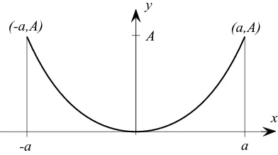
The simplest example of a variational principle is that of finding the shortest distance between two points. Suppose the two points lie in a plane, with one point at the origin, O, and the other at pointA with coordinates (1,1), then if y(x) represents a smooth curve passing throughOandAthe distance betweenOandA, along this curve is given by the functional defined in equation 1.1. The shortest path is that which minimises the value ofS[y]. If the surface is curved, for instance a sphere or ellipsoid, the equivalent functional is more complicated, but the shortest path is that which minimises it.
Variational principles are important for three principal reasons. First, many prob-lems are naturally formulated in terms of a functional and an associated variational principle. Several of these will be described in chapter 2 and some solutions will be obtained as the course develops.
Second, most equations of mathematical physics can be derived from variational principles. This is important partly because it suggests a unifying theme in our descrip-tion of nature and partly because such formuladescrip-tions are independent of any particular coordinate system, so making the essential mathematical structure of the equations more transparent and easier to understand. This aspect of the subject is not consid-ered in this course; a good discussion of these problems can be found in Yourgrau and Mandelstam (1968)2.
Finally, variational principles provide powerful computational tools; we explore as-pects of this theory in chapter 12.
Consider the problem of finding the shortest path between two points on a curved surface. The associated functional assigns a real number to each smooth curve joining the points. A first step to solving this problem is to find the stationary values of the functional; it is then necessary to decide which of these provides the shortest path. This is very similar to the problem of finding extreme values of a function of n variables, where we first determine the stationary points and then classify them: the important and significant difference is that the space of allowed functions is not usually finite in dimension. The infinite dimensional spaces of functions, with which we shall be dealing, has many properties similar to those possessed by finite dimensional spaces, and in the many problems the difference is not significant. However, this generalisation does introduce some practical and technical difficulties some of which are discussed in section 3.6. In this chapter we review calculus in order to prepare for these more general ideas of calculus.
In elementary calculus and analysis, the functions studied first are ‘real functions,f, of one real variable’, that is, functions with domain either R, or a subset of R, and codomainR. Without any other restrictions on f, this definition is too general to be useful in calculus and applied mathematics. Most functions of one real variable that are of interest in applications have smooth graphs, although sometimes they may fail to be smooth at one or more points where they have a ‘kink’ (fail to be differentiable), or even a break (where they are discontinuous). This smooth behaviour is related to
2Yourgrau W and Mandelstram SVariational Principles in Dynamics and Quantum Theory
1.1. INTRODUCTION 11 the fact that most important functions of one variable describe physical phenomena and often arise as solutions of ordinary differential equations. Therefore it is usual to restrict attention to functions that are differentiable or, more usually, differentiable a number of times.
The most useful generalisation of differentiability to functions defined on sets other thanR requires some care. It is not too hard in the case of functions of several (real) variables but we shall have to generalise differentiation and integration tofunctionals, not just to functions of several real variables.
Our presentation conceals very significant intellectual achievements made at the end of the nineteenth century and during the first half of the twentieth century. During the nineteenth century, although much work was done on particular equations, there was little systematic theory. This changed when the idea of infinite dimensional vector spaces began to emerge. Between 1900 and 1906, fundamental papers appeared by Fredholm3, Hilbert4, and Fr´echet5. Fr´echet’s thesis gave for the first time definitions of
limit and continuity that were applicable in very general sets. Previously, the concepts had been restricted to special objects such as points, curves, surfaces or functions. By introducing the concept of distance in more general sets he paved the way for rapid advances in the theory of partial differential equations. These ideas together with the theory of Lebesgue integration introduced in 1902, by Lebesgue in his doctoral thesis6,
led to the modern theory of functional analysis. This is now the usual framework of the theoretical study of partial differential equations. They are required also for an elucidation of some of the difficulties in the Calculus of Variations. However, in this introductory course, we concentrate on basic techniques of solving practical problems, because we think this is the best way to motivate and encourage further study.
This preliminary chapter, which is assessed, is about real analysis and introduces many of the ideas needed for our treatment of the Calculus of Variations. It is possible that you are already familiar with the mathematics described in this chapter, in which case you could start the course with chapter 2. You should ensure, however, that you have a good working knowledge of differentiation, both ordinary and partial, Taylor series of one and several variables and differentiation under the integral sign, all of which are necessary for the development of the theory. In addition familiarity with the theory of linear differential equations with both initial and boundary value problems is assumed.
Very many exercises are set, in the belief that mathematical ideas cannot be un-derstood without attempting to solve problems at various levels of difficulty and that one learns most by making one’s own mistakes, which is time consuming. You should not attempt all these exercise at a first reading, but these provide practice of essential mathematical techniques and in the use of a variety of ideas, so you should do as many as time permits; thinking about a problem, then looking up the solution is usually of
3I. Fredholm, On a new method for the solution of Dirichlet’s problem, reprinted in Oeuvres
Compl`etes, l’Institut Mittag-Leffler, (Malm¨o) 1955, pp 61-68 and 81-106
4D. Hilbert published six papers between 1904 and 1906. They were republished as Grundz¨uge
einer allgemeinen Theorie der Integralgleichungenby Teubner, (Leipzig and Berlin), 1924. The most crucial paper is the fourth.
5M. Fr´echet, Doctoral thesis,Sur quelques points du Calcul fonctionnel, Rend. Circ. mat. Palermo
22 (1906), pp 1-74.
6H. Lebesgue, Doctoral thesis, Paris 1902, reprinted in Annali Mat. pura e appl., 7 (1902) pp
little value until you have attempted your own solution. The exercises at the end of this chapter are examples of the type of problem that commonly occur in applications: they are provided for extra practice if time permits and it is not necessary for you to attempt them.
1.2
Notation and preliminary remarks
We start with a discussion about notation and some of the basic ideas used throughout this course.
A real function of a single real variable, f, is a rule that maps a real number x to a single real numbery. This operation can be denoted in a variety of ways. The approach of scientists is to write y = f(x) or just y(x), and the symbols y, y(x), f and f(x) are all used to represent the function. Mathematics uses the more formal and precise notation f
:
X →Y, where X and Y are subsets of the real line: the set X is named the domain, or the domain of definition of f, and set Y the codomain. With this notation the symbol f denotes the function and the symbol f(x) the value of the function at the point x. In applications this distinction is not always made and both f and f(x) are used to denote the function. In recent years this has come to be regarded as heresy by some: however, there are good practical reasons for using this freer notation that do not affect pure mathematics. In this text we shall frequently use the Leibniz notation, f(x), and its extensions, because it generally provides a clearer picture and is helpful for algebraic manipulations, such as when changing variables and integrating by parts.Moreover, in the sciences the domain and codomain are frequently omitted, either because they are ‘obvious’ or because they are not known. But, perversely, the scientist, by writingy =f(x), often distinguishes between the two variablesxandy, by saying thatxis theindependentvariable and thatyis thedependentvariable because it depends uponx. This labelling can be confusing, because the role of variables can change, but it is also helpful because in physical problems different variables can play quite different roles: for instance, time is normally an independent variable.
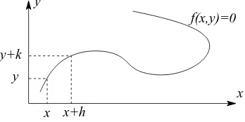
In pure mathematics the termgraphis used in a slightly specialised manner. A graph is the set of points (x, f(x)): this is normally depicted as a line in a plane using rect-angular Cartesian coordinates. In other disciplines the whole figure is called the graph, not the set of points, and the graph may be a less restricted shape than those defined by functions; an example is shown in figure 1.5 (page 30).
Almost all the ideas associated with real functions of one variable generalise to functions of several real variables, but notation needs to be developed to cope with this extension. Points in Rn are represented by n-tuples of real numbers (x1, x2, . . . , xn).
It is convenient to use bold faced symbols, x, a and so on, to denote these points, so x = (x1, x2, . . . , xn) and we shall write x and (x1, x2, . . . , xn) interchangeably. In
hand-written text a bold character,x, is usually denoted by an underline,x.
A functionf(x1, x2, . . . , xn) ofnreal variables, defined onRn, is a map fromRn, or a
subset, toR, written asf
:
Rn→R. Where we use bold face symbols likef orφ
to referto functions, it means that theimageunder the functionf(x) or
φ(
y) may be considered as vector inRmwithm≥2, sof:
Rn→Rm; in this course normallym= 1 orm=n.1.2. NOTATION AND PRELIMINARY REMARKS 13 valued. We shall also write without further comment f(x) = (f1(x), f2(x), . . . , fm(x)),
so that the fi are the mcomponent functions,fi
:
Rn→R, off.On the real line the distance between two points x and y is naturally defined by
|x−y|. A pointxis in theopen interval(a, b) ifa < x < b, and is in theclosed interval [a, b] if a≤x≤b. By convention, the intervals (−∞, a),(b,∞) and (−∞,∞) =R are also open intervals. Here, (−∞, a) means the set of all real numbers strictly less than a. The symbol ∞ for ‘infinity’ is not a number, and its use here is conventional. In the language and notation of set theory, we can write (−∞, a) ={x∈R:x < a},with similar definitions for the other two types of open interval. One reason for considering open sets is that the natural domain of definition of some important functions is an open set. For example, the function lnxas a function of one real variable is defined for x∈(0,∞).
The space of pointsRn is an example of a linear space. Here the term linearhas
the normal meaning that for every x,yin Rn, and for every realα,x+yandαxare
in Rn. Explicitly,
(x1, x2, . . . , xn) + (y1, y2, . . . , yn) = (x1+y1, x2+y2,· · · , xn+yn)
and
α(x1, x2, . . . , xn) = (αx1, αx2, . . . , αxn).
Functions f
:
Rn→Rm may also be added and multiplied by real numbers. Thereforea function of this type may be regarded as a vector in the vector space of functions — though this space is not finite dimensional likeRn.
In the spaceRn the distance|x| of a pointxfrom the origin is defined by the
nat-ural generalisation of Pythagoras’ theorem, |x| = px2
1+x22+· · ·+x2n. The distance
between two vectorsxandyis then defined by
|x−y|= q
(x1−y1)2+ (x2−y2)2+· · ·+ (xn−yn)2. (1.2)
This is a direct generalisation of the distance along a line, to which it collapses when n= 1.
This distance has the three basic properties (a) |x| ≥0 and |x|= 0 if and only if x= 0, (b) |x−y|=|y−x|,
(c) |x−y|+|y−z| ≥ |x−z|, (Triangle inequality).
(1.3)
In the more abstract spaces, such as the function spaces we need later, a similar concept of a distance between elements is needed. This is named the normand is a map from two elements of the space to the positive real numbers and which satisfies the above three rules. In function spaces there is no natural choice of the distance function and we shall see in chapter 3 that this flexibility can be important.
For functions of several variables, that is, for functions defined on sets of points in Rn, the direct generalization of open interval is anopen ball.
Definition 1.1
Thus the ball of radius 1 and centre (0,0) in R2 is the interior of the unit circle, not
including the points on the circle itself. And in R, the ‘ball’ of radius 1 and centre 0 is the open interval (−1,1). However, forR2 and forRn forn >2, open balls are not
quite general enough. For example, the open square
{(x, y)∈R2:|x|<1,|y|<1}
is not a ball, but in many ways is similar. (You may know for example that it may be mapped continuously to an open ball.) It turns out that the most convenient concept is that of open set7, which we can now define.
Definition 1.2
Open sets. A set U inRn is said to be openif for everyx∈U there is an open ball Br(a) wholly contained withinU which containsx.
In other words, every point in an open set lies in an open ball contained in the set. Any open ball is in many ways like the whole of the spaceRn — it has no isolated or
missing points. Also, every open set is a union of open balls (obviously). Open sets are very convenient and important in the theory of functions, but we cannot study the reasons here. A full treatment of open sets can be found in books on topology8. Open
balls are not the only type of open sets and it is not hard to show that the open square,
{(x, y)∈R2:|x|<1,|y|<1}, is in fact an open set, according to the definition we gave;
and in a similar way it can be shown that the set{(x, y)∈R2 : (x/a)2+ (y/b)2<1}, which is the interior of an ellipse, is an open set.
Exercise 1.1
Show that the open square is an open set by constructing explicitly for each (x, y) in the open square{(x, y) ∈ R2 : |x|< 1,|y|< 1} a ball containing (x, y) and
lying in the square.
1.2.1
The Order notation
It is often useful to have a bound for the magnitude of a function that does not require exact calculation. For example, the function f(x) = p
sin(x2coshx)−x2cosxtends
to zero at a similar rate tox2 asx→0 and this information is sometimes more helpful
than the detailed knowledge of the function. The order notation is designed for this purpose.
Definition 1.3
Order notation. A function f(x) is said to be of order xn as x → 0 if there is a
non-zero constant C such that |f(x)| < C|xn| for allx in an interval around x = 0.
This is written as
f(x) =O(xn) as x→0. (1.4)
The conditional clause ‘as x→ 0’ is often omitted when it is clear from the context. More generally, this order notation can be used to compare the size of functions, f(x)
7As with many other concepts in analysis, formulating clearly the concepts, in this case an open
set, represents a major achievement.
8See for example W A Sutherland,Introduction to Metric and Topological Spaces, Oxford University
1.2. NOTATION AND PRELIMINARY REMARKS 15 and g(x): we say that f(x) is of the order of g(x) as x → y if there is a non-zero constantCsuch that|f(x)|< C|g(x)|for allxin an interval aroundy; more succinctly, f(x) =O(g(x)) asx→y.
When used in the form f(x) = O(g(x)) as x → ∞, this notation means that
|f(x)| < C|g(x)| for all x > X, where X and C are positive numbers independent ofx.
This notation is particularly useful when truncating power series: thus, the series for sinxup toO(x3) is written,
sinx=x−x
3
3! +O(x
5),
meaning that the remainder is smaller than C|x|5, asx→0 for some C. Note that in
this course the phrase “up toO(x3)” means that thex3term isincluded. The following
exercises provide practice in using theO-notation and exercise 1.2 proves an important result.
Exercise 1.2
Show that iff(x) =O(x2) asx→0 then alsof(x) =O(x).
Exercise 1.3
Use the binomial expansion to find the order of the following expressions asx→0.
(a) xp1 +x2, (b) x
1 +x, (c) x3/2
1−e−x.
Exercise 1.4
Use the binomial expansion to find the order of the following expressions asx→ ∞.
(a) x
x−1, (b)
p
4x2+x−2x, (c) (x+b)a
−xa, a >0.
The order notation is usefully extended to functions of n real variables,f
:
Rn →R,by using the distance |x|. Thus, we say that f(x) = O(|x|n) if there is a non-zero constant Cand a small numberδsuch that|f(x)|< C|x|n for|x|< δ.
Exercise 1.5
(a) Iff1 =xand f2 = yshow that f1 =O(f) and f2 =O(f) where f(x, y) =
(x2+y2)12.
(b) Show that the polynomialφ(x, y) =ax2+bxy+cy2 vanishes to at least the
same order as the polynomialf(x, y) =x2+y2 at (0,0). What conditions are
needed forφto vanish faster thanf as p
x2+y2→0?
Another expression that is useful is
f(x) =o(|x|) which is shorthand for lim |x|→0
f(x)
|x| = 0.
Informally this means that f(x) vanishes faster than |x| as |x| → 0. More generally f =o(g) if lim|x|→0|f(x)/g(x)| = 0, meaning that f(x) vanishes faster than g(x) as
1.3
Functions of a real variable
1.3.1
Introduction
In this section we introduce important ideas pertaining to real functions of a single real variable, although some mention is made of functions of many variables. Most of the ideas discussed should be familiar from earlier courses in elementary real analysis or Calculus, so our discussion is brief and all exercises are optional.
The study of Real Analysis normally starts with a discussion of the real number system and its properties. Here we assume all necessary properties of this number system and refer the reader to any basic text if further details are required: adequate discussion may be found in the early chapters of the texts by Whittaker and Watson9,
Rudin10 and by Kolmogorov and Fomin11.
1.3.2
Continuity and Limits
A continuousfunction is one whose graph has no vertical breaks: otherwise, it is dis-continuous. The function f1(x), depicted by the solid line in figure 1.1 is continuous
for x1 < x < x2. The functionf2(x), depicted by the dashed line, is discontinuous at x=c.
x
( )
f2
x
( )
f2 x
( )
f1 y
x
x1 c x2
Figure 1.1 Figure showing examples of a continuous function,f1(x), and a discontinuous functionf2(x).
A functionf(x) is continuous at a pointx=aiff(a) exists and if, given any arbitrarily small positive number,ǫ, we can find a neighbourhood ofx=asuch that in it|f(x)−
f(a)|< ǫ. We can express this in terms of limits and since a point aon the real line can be approached only from the left or the right a function is continuous at a point x=aif it approaches the same value, independent of the direction. Formally we have Definition 1.4
Continuity: a function,f, is continuous atx=aiff(a) is defined and lim
x→af(x) =f(a).
For a function of one variable, this is equivalent to saying that f(x) is continuous at x=aiff(a) is defined and the left and right-hand limits
lim
x→a−
f(x) and lim
x→a+ f(x),
9A Course of Modern Analysisby E T Whittaker and G N Watson, Cambridge University Press. 10Principles of Mathematical Analysisby W Rudin (McGraw-Hill).
1.3. FUNCTIONS OF A REAL VARIABLE 17 exist andare equal tof(a).
If the left and right-hand limits exist but arenotequal the function is discontinuous atx=aand is said to have asimplediscontinuity atx=a.
If they both exist and are equal, but do not equalf(a), then the function is said to have aremovablediscontinuity atx=a.
Quite elementary functions exist for which neither limit exists: these are also dis-continuous, and said to have a discontinuity of the second kind at x= a, see Rudin (1976, page 94). An example of a function with such a discontinuity at x= 0 is
f(x) =
sin(1/x), x6= 0, 0, x= 0.
We shall have no need to consider this type of discontinuity in this course, but simple discontinuities will arise.
A function that behaves as
|f(x+ǫ)−f(x)|=O(ǫ) as ǫ→0
is continuous, though the converse is not true, a counter example beingf(x) =p|x|at x= 0.
Most functions that occur in the sciences are either continuous orpiecewise continu-ous, which means that the function is continuous except at a discrete set of points. The Heaviside function and the related sgn functions are examples of commonly occurring piecewise continuous functions that are discontinuous. They are defined by
H(x) =
1, x >0,
0, x <0, and sgn(x) =
1, x >0,
−1, x <0, sgn(x) =−1 + 2H(x). (1.5) These functions are discontinous at x = 0, where they are not normally defined. In some texts these functions are defined at x= 0; for instance H(0) may be defined to have the value 0, 1/2 or 1.
If limx→cf(x) =A and limx→cg(x) =B, then it can be shown that the following
(obvious) rules are adhered to: (a) lim
x→c(αf(x) +βg(x)) =αA+βB;
(b) lim
x→c(f(x)g(x)) =AB;
(c) lim
x→c f(x) g(x) =
A
B,ifB6= 0; (d) if lim
x→Bf(x) =fB then limx→c(f(g(x)) =fB.
The value of a limit is normally found by a combination of suitable re-arrangements and expansions. An example of an expansion is
lim
x→0
sinhax x = limx→0
ax+3!1(ax)3+O(x5) x = limx→0
a+O(x2)=a. An example of a re-arrangement, using the above rules, is
lim
x→0
sinhax sinhbx = limx→0
sinhax x
x
sinhbx = limx→0
sinhax x xlim→0
x sinhbx =
a
Finally, we note that a function that is continuous on a closed interval is bounded above and below and attains its bounds. It is important that the interval is closed; for instance the functionf(x) =xdefined in the open interval 0< x <1 is bounded above and below, but does not attain it bounds. This example may seem trivial, but similar difficulties exist in the Calculus of Variations and are less easy to recognise.
Exercise 1.6
A function that is finite and continuous for allxis defined by
f(x) =
8 > > <
> > :
A
x2 +x+B, 0≤x≤a, a >0,
C
x2 +Dx, a≤x,
whereA,B,C,D andaare real numbers: iff(0) = 1 and limx→∞f(x) = 0, find
these numbers.
Exercise 1.7
Find the limits of the following functions asx→0 andw→ ∞.
(a) sinax
x , (b)
tanax
x , (c)
sinax sinbx, (d)
3x+ 4 4x+ 2, (e)
“
1 + z w
”w
.
For functions of two or more variables, the definition of continuity is essentially the same as for a function of one variable. A functionf(x) is continuous atx=a iff(a) is defined and
lim x→af(
x) =f(a). (1.6)
Alternatively, given any ǫ > 0 there is a δ > 0 such that whenever |x −a| < δ,
|f(x)−f(a)|< ǫ.
It should be noted that iff(x, y) is continuous ineachvariable, it is not necessarily continuous in both variables. For instance, consider the function
f(x, y) =
(x+y)2 x2+y2, x
2+y2
6
= 0, 1, x=y= 0, and for fixedy=β6= 0 the related function of x,
f(x, β) = (x+β)
2
x2+β2 = 1 +O(x) as x→0
andf(x,0) = 1 for allx: for any β this function is a continuous function ofx. On the line x+y = 0, however,f = 0 except at the origin so f(x, y) is not continuous along this line. More generally, by putting x=rcosθ andy =rsinθ,−π < θ≤π,r6= 0, we can approach the origin from any angle. In this representationf = 2 sin2θ+π
4
so on any circle round the originf takes any value between 0 and 2. Thereforef(x, y) is not a continuous function of bothxandy.
Exercise 1.8
Determine whether or not the following functions are continuous at the origin.
(a)f= 2xy
x2+y2, (b)f=
x2+y2
x2−y2, (c)f =
2x2y
x2+y2.
1.3. FUNCTIONS OF A REAL VARIABLE 19
1.3.3
Monotonic functions and inverse functions
A function is said to be monotonic on an interval if it is always increasing or always decreasing. Simple examples are f(x) = x and f(x) = exp(−x) which are mono-tonic increasing and monomono-tonic decreasing, respectively, on the whole line: the function f(x) = sinxis monotonic increasing for−π/2< x < π/2. More precisely, we have, Definition 1.5
Monotonic functions: A functionf(x) ismonotonicincreasing fora < x < bif f(x1)≤f(x2) for a < x1< x2< b.
A monotonic decreasing function is defined in a similar way.
Iff(x1)< f(x2) fora < x1< x2< bthenf(x) is said to bestrictly monotonic
(in-creasing) orstrictly increasing; strictly decreasing functions are defined in the obvious manner.
The recognition of the intervals on which a given function is strictly monotonic is sometimes important because on these intervals the inverse function exists. For instance the functiony=exis monotonic increasing on the whole real line,R, and its inverse is
the well known natural logarithm,x= lny, withy on the positive real line.
In general iff(x) is continuous and strictly monotonic ona≤x≤b andy=f(x) the inverse function, x = f−1(y), is continuous for f(a) ≤ y ≤ f(b) and satisfies y=f(f−1(y)). Moreover, iff(x) is strictly increasing so is f−1(y).
Complications occur when a function is increasing and decreasing on neighbouring intervals, for then the inverse may have two or more values. For example the function f(x) =x2is monotonic increasing forx >0 and monotonic decreasing forx <0: hence
the relationy=x2has the two familiar inversesx=±√y,y≥0. These two inverses are
often refered to as the different branchesof the inverse; this idea is important because most functions are monotonic only on part of their domain of definition.
Exercise 1.9
(a) Show thaty= 3a2x−x3is strictly increasing for−a < x < aand that on this
intervalyincreases from−2a3 to 2a3.
(b) By puttingx = 2asinφ and using the identity sin3φ = (3 sinφ−sin 3φ)/4, show that the equation becomes
y= 2a3sin 3φ and hence that x(y) = 2asin
„
1 3sin
−1“ y
2a3
”«
.
(c) Find the inverse for x > 2a. Hint put x = 2acoshφ and use the relation cosh3φ= (cosh 3φ+ 3 coshφ)/4.
1.3.4
The derivative
Q
P
a
f(a+h)
f(a)
a+h
φ
Tangentat PFigure 1.2 Illustration showing the chordP Qand the tan-gent line atP.
The gradient of the chordP Qis tanφwhereφis the angle betweenP Qand thex-axis, and is given by the formula
tanφ= f(a+h)−f(a)
h .
If the graph in the vicinity ofx=ais represented by a smooth line, then it is intuitively obvious that the chordP Q becomes closer to the tangent atP as h→0; and in the limith= 0 the chord becomes the tangent. Hence the gradient of the tangent is given by the limit
lim
h→0
f(a+h)−f(a)
h .
This limit, provided it exists, is named the derivative off(x) atx=aand is commonly denoted either byf′(a) or df
dx. Thus we have the formal definition:
Definition 1.6
The derivative: A function f(x), defined on an open interval U of the real line, is differentiable forx∈U and has thederivativef′(x) if
f′(x) = df dx = limh→0
f(x+h)−f(x)
h , (1.7)
exists.
If the derivative exists at every point in the open intervalU the functionf(x) is said to be differentiable in U: in this case it may be proved that f(x) is also continuous. However, a function that is continuous at a need not be differentiable at a: indeed, it is possible to construct functions that are continuous everywhere but differentiable nowhere; such functions are encountered in the mathematical description of Brownian motion.
Combining the definition off′(x) and the definition 1.3 of the order notation shows that a differentiable function satisfies
1.3. FUNCTIONS OF A REAL VARIABLE 21 The tangent line to the graphy =f(x) at the point a, which we shall consider to be fixed for the moment, has slope f′(a) and passes through f(a). These two facts determine the derivative completely. The equation of the tangent line can be written in parametric form as p(h) = f(a) +f′(a)h. Conversely, given a point a, and the equation of the tangent line at that point, the derivative, in the classical sense of the definition 1.6, is simply the slope, f′(a), of this line. So the information that the derivative of f at a is f′(a) is equivalent to the information that the tangent line at
a has equationp(h) =f(a) +f′(a)h. Although the classical derivative, equation 1.7, is usually taken to be the fundamental concept, the equivalent concept of the tangent line at a point could be considered equally fundamental - perhaps more so, since a tangent is a more intuitive idea than the numerical value of its slope. This is the key to successfully defining the derivative of functions of more than one variable.
From the definition 1.6 the following useful results follow. If f(x) and g(x) are differentiable on the same open interval andαandβ are constants then
(a) d dx
αf(x) +βg(x)=αf′(x) +βg′(x), (b) d
dx
f(x)g(x)=f′(x)g(x) +f(x)g′(x), (The product rule) (c) d
dx
f(x) g(x)
=f
′(x)g(x)−f(x)g′(x)
g(x)2 , g(x)6= 0. (The quotient rule)
We leave the proof of these results to the reader, but note that the differential of 1/g(x) follows almost trivially from the definition 1.6, exercise 1.14, so that the third expression is a simple consequence of the second.
The other important result is thechain ruleconcerning the derivative of composite functions. Suppose that f(x) and g(x) are two differentiable functions and a third is formed by the composition,
F(x) =f(g(x)), sometimes written as F =f◦g,
which we assume to exist. Then the derivative ofF(x) can be shown, as in exercise 1.18, to be given by
dF dx =
df dg ×
dg
dx or F
′(x) =f′(g)g′(x). (1.9) This formula is named thechain rule. Note how the prime-notation is used: it denotes the derivative of the function with respect to the argument shown, not necessarily the original independent variable, x. Thusf′(g) orf′(g(x)) does not mean the derivative ofF(x); it means the derivativef′(x) withxreplaced bygor g(x).
A simple example should make this clear: supposef(x) = sinxand g(x) = 1/x, x >0, soF(x) = sin(1/x). The chain rule gives
dF dx =
d
dg(sing)× d dx
1
x
= cosg×
− 1
x2
=−1
x2cos
1
x
.
Exercise 1.10
Find the derivative of the following functions
(a) p
(a−x)(b+x) , (b) pasin2x+bcos2x, (c) cos(x3) cosx, (d) xx.
Exercise 1.11
Ify= sinxfor−π/2≤x≤π/2 show that dx dy =
1
p
1−y2.
Exercise 1.12
(a) Ify=f(x) has the inversex=g(y), show thatf′
(x)g′
(y) = 1, that is
dx dy =
„dy
dx
«−1
.
(b) Express d
2x
dy2 in terms of
dy dx and
d2y
dx2.
Clearly, iff′(x) is differentiable, it may be differentiated to obtain the second derivative, which is denoted by
f′′(x) or d
2f dx2.
This process can be continued to obtain the functions
f, df
dx, d2f dx2,
d3f dx3,· · · ,
dn−1f dxn−1,
dnf dxn · · ·,
where each member of the sequence is the derivative of the preceeding member, dpf
dxp = d dx
dp−1f dxp−1
, p= 2,3,· · ·.
The prime notation becomes rather clumsy after the second or third derivative, so the most common alternative is
dpf dxp =f
(p)(x), p≥2,
with the conventionsf(1)(x) =f′(x) andf(0)(x) =f(x). Care is needed to distinguish
between thepth derivative,f(p)(x), and thepth power, denoted byf(x)pand sometimes fp(x) — the latter notation should be avoided if there is any danger of confusion.
Functions for which thenth derivative is continuous are said to be n-differentiable and to belong to classCn: the notationCn(U) means the firstnderivatives are
continu-ous on the intervalU: the notationCn(a, b) orCn[a, b], with obvious meaning, may also
be used. The term smooth functiondescribes functions belonging to C∞, that is func-tions, such as sinx, having all derivatives; we shall, however, use the termsufficiently smooth for functions that are sufficiently differentiable for all subsequent analysis to work, when more detail is deemed unimportant.
1.3. FUNCTIONS OF A REAL VARIABLE 23 Exercise 1.13
Iff(x) is an even (odd) function, show thatf′
(x) is an odd (even) function.
Exercise 1.14
Show, from first principles using the limit 1.7, that d dx
„
1 f(x)
«
=−f
′
(x) f(x)2, and
that the product rule is true.
Exercise 1.15
Leibniz’s rule
Ifh(x) =f(x)g(x) show that
h′′(x) = f′′(x)g(x) + 2f′(x)g′(x) +f(x)g′′(x),
h(3)(x) = f(3)(x)g(x) + 3f′′(x)g′(x) + 3f′(x)g′′(x) +f(x)g(3)(x), and use induction to deriveLeibniz’s rule
h(n)(x) =
n
X
k=0
„
n k
«
f(n−k)(x)g(k)(x),
where the binomial coefficients are given by
„
n k
«
= n!
k! (n−k)!.
Exercise 1.16
Show that d
dxln(f(x)) = f′(x)
f(x) and hence that if
p(x) =f1(x)f2(x)· · ·fn(x) then p
′
p =
f1′
f1
+f
′ 2
f2
+· · ·+f
′
n
fn
,
providedp(x)6= 0. Note that this gives an easier method of differentiating prod-ucts of three or more factors than repeated use of the product rule.
Exercise 1.17
If the elements of a determinantD(x) are differentiable functions ofx,
D(x) =
˛ ˛ ˛ ˛
f(x) g(x)
φ(x) ψ(x)
˛ ˛ ˛ ˛
show that
D′(x) =
˛ ˛ ˛ ˛
f′
(x) g′
(x)
φ(x) ψ(x)
˛ ˛ ˛ ˛
+
˛ ˛ ˛ ˛
f(x) g(x)
φ′
(x) ψ′
(x)
˛ ˛ ˛ ˛
.
1.3.5
Mean Value Theorems
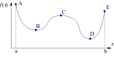
If a function f(x) is sufficiently smooth for all points inside the interval a < x < b, its graph is a smooth curve12 starting at the point A = (a, f(a)) and ending at B =
(b, f(b)), as shown in figure 1.3.
B
A Q
P
a b
f(a) f(b)
Figure 1.3 Diagram illustrating Cauchy’s form of the mean value theorem.
From this figure it seems plausible that the tangent to the curve must be parallel to the chordAB at least once. That is
f′(x) = f(b)−f(a)
b−a for somexin the intervala < x < b. (1.10) Alternatively this may be written in the form
f(b) =f(a) +hf′(a+θh), h=b−a. (1.11)
whereθ is a number in the interval 0< θ <1, and is normally unknown. This relation is used frequently throughout the course. Note that equation 1.11 shows that between zeros of a continuous function there is at least one point at which the derivative is zero. Equation 1.10 can be proved and is enshrined in the following theorem
Theorem 1.1
The Mean Value Theorem(Cauchy’s form). Iff(x) andg(x) are real and differen-tiable for a≤x≤b, then there is a pointuinside the interval at which
f(b)−f(a)g′(u) =g(b)−g(a)f′(u), a < u < b. (1.12)
By putting g(x) =x, equation 1.10 follows.
A similar idea may be applied to integrals. In figure 1.4 is shown a typical continuous function, f(x), which attains its smallest and largest values,S andL respectively, on the intervala≤x≤b.
12A smooth curve is one along which its tangent changes direction continuously, without abrupt
1.3. FUNCTIONS OF A REAL VARIABLE 25
a b
f(x) S
L
Figure 1.4 Diagram showing the upper and lower bounds off(x) used to bound the integral.
It is clear that the area under the curve is greater than (b−a)Sand less than (b−a)L, that is
(b−a)S≤
Z b
a
dx f(x)≤(b−a)L. Becausef(x) is continuous it follows that
Z b
a
dx f(x) = (b−a)f(ξ) for someξ∈[a, b]. (1.13)
This observation is made rigorous in the following theorem. Theorem 1.2
The Mean Value theorem(integral form). If, on the closed intervala≤x≤b,f(x) is continuous andφ(x)≥0 then there is anξ satisfyinga≤ξ≤bsuch that
Z b
a
dx f(x)φ(x) =f(ξ) Z b
a
dx φ(x). (1.14)
Ifφ(x) = 1 relation 1.13 is regained.
Exercise 1.18
The chain rule
In this exercise the Mean Value Theorem is used to derive the chain rule, equa-tion 1.9, for the derivative ofF(x) =f(g(x)).
Use the mean value theorem to show that
F(x+h)−F(x) =f“g(x) +hg′(x+hθ)”−f(g(x)) and that
f“g(x) +hg′(x+hθ)”=f(g(x)) +hg′(x+hθ)f′(g+hφg′) where 0< θ, φ <1. Hence show that
F(x+h)−F(x)
h =f
′
Exercise 1.19
Use the integral form of the mean value theorem, equation 1.13, to evaluate the limits,
(a) lim
x→0
1 x
Zx
0
dtp4 + 3t3, (b) lim
x→1
1 (x−1)3
Z x
1
dtln`
3t−3t2+t3´
.
1.3.6
Partial Derivatives
Here we consider functions of two or more variables, in order to introduce the idea of a partial derivative. If f(x, y) is a function of the two, independent variables x and y, meaning that changes in one do not affect the other, then we may form the partial derivative of f(x, y) with respect to either x or y using a minor modification of the definition 1.6 (page 20).
Definition 1.7
The partial derivativeof a function f(x, y) of two variables with respect to the first variablexis
∂f
∂x =fx(x, y) = limh→0
f(x+h, y)−f(x, y)
h .
In the computation offx the variabley is unchanged.
Similarly, the partial derivative with respect to the second variabley is ∂f
∂y =fy(x, y) = limk→0
f(x, y+k)−f(x, y)
k .
In the computation offy the variablexis unchanged.
We use the conventional notation,∂f /∂x, to denote the partial derivative with respect tox, which is formed by fixingyand using the rules of ordinary calculus for the deriva-tive with respect tox. The suffix notation,fx(x, y), is used to denote the same function:
here the suffix xshows the variable being differentiated, and it has the advantage that when necessary it can be used in the formfx(a, b) to indicate that the partial derivative fxis being evaluated at the point (a, b).
In practice the evaluation of partial derivatives is exactly the same as ordinary derivatives and the same rules apply. Thus iff(x, y) =xeyln(2x+ 3y) then the partial
derivatives with respect toxand yare, repectively ∂f
∂x =e
yln(2x+ 3y) + 2xey
2x+ 3y and ∂f ∂y =xe
yln(2x+ 3y) + 3xey
2x+ 3y.
Exercise 1.20
(a) Ifu=x2sin(lny) computeuxanduy.
(b) Ifr2=x2+y2 show that ∂r
∂x= x r and
∂r ∂y =
y r.
The partial derivatives are also functions of xand y, so may be differentiated again. Thus we have
∂ ∂x
∂f
∂x
= ∂
2f
∂x2 =fxx(x, y) and ∂ ∂y
∂f
∂y
= ∂
2f
1.3. FUNCTIONS OF A REAL VARIABLE 27 But now we also have the mixed derivatives
∂ ∂x
∂f ∂y
and ∂
∂y
∂f ∂x
. (1.16)
Except in special circumstances the order of differentiation is irrelevant so we obtain themixed derivative rule
∂ ∂x
∂f
∂y
= ∂
∂y
∂f
∂x
= ∂
2f ∂x∂y =
∂2f
∂y∂x. (1.17)
Using the suffix notation the mixed derivative rule is fxy = fyx. A sufficient
condi-tion for this to hold is that both fxy and fyx are continuous functions of (x, y), see
equation 1.6 (page 18).
Similarly, differentiatingptimes with respect toxandqtimes with respect to y, in any order, gives the samenth order derivative,
∂nf
∂xp∂yq where n=p+q,
provided all thenth derivatives are continuous. Exercise 1.21
If Φ(x, y) = exp(−x2/y) show that Φ satisfies the equations
∂Φ ∂x =−
2xΦ
y and
∂2Φ
∂x2 = 4
∂Φ ∂y −
2Φ y .
Exercise 1.22
Show thatu=x2sin(lny) satisfies the equation 2y2∂
2u
∂y2 + 2y
∂u ∂y +x
∂u ∂x = 0.
The generalisation of these ideas to functions of thenvariablesx= (x1, x2, . . . , xn) is
straightforward: the partial derivative of f(x) with respect to xk is defined to be ∂f
∂xk
= lim
h→0
f(x1, x2,· · ·, xk−1, xk+h, xk+1,· · ·, xn)−f(x1, x2, . . . , xn)
h . (1.18)
All other properties of the derivatives are the same as in the case of two variables, in particular for themth derivative the order of differentiation is immaterial provided all mth derivatives are continuous.
For a function of a single variable, f(x), the existence of the derivative, f′(x), implies thatf(x) is continuous. For functions of two or more variables the existence of the partial derivatives does not guarantee continuity.
The total derivative
Iff(x1, x2, . . . , xn) is a function ofnvariables and if each of these variables is a function
of the single variable t, we may form a new function oft with the formula
Geometrically,F(t) represents the value off(x) on a curveCdefined parametrically by the functions (x1(t), x2(t),· · · , xn(t)). The derivative ofF(t) is given by the relation
dF dt =
n
X
k=1 ∂f ∂xk
dxk
dt , (1.20)
so F′(t) is the rate of change of f(x) along C. Normally, we write f(t) rather than use a different symbolF(t), and the left-hand side of the above equation is written df
dt. This derivative is named the total derivative off. The proof of this when n = 2 and x′ and y′ do not vanish near (x, y) is sketched below; the generalisation to largern is straightforward. IfF(t) =f(x(t), y(t)) then
F(t+ǫ) = f(x(t+ǫ), y(t+ǫ))
= fx(t) +ǫx′(t+θǫ), y(t) +ǫy′(t+φǫ), 0< θ, φ <1,
where we have used the mean value theorem, equation 1.11. Write the right-hand side in the form
f(x+ǫx′, y+ǫy′) =hf(x+ǫx′, y+ǫy′)−f(x, y+ǫy′)i+hf(x, y+ǫy′)−f(x, y)i+f(t) so that
F(t+ǫ)−F(t)
ǫ =
f(x+ǫx′, y+ǫy′)−f(x, y+ǫy′)
ǫx′ x′+
f(x, y+ǫy′)−f(x, y)
ǫy′ y′.
Thus, on taking the limit asǫ→0 we have dF
dt = ∂f ∂x
dx dt +
∂f ∂y
dy dt.
This result remains true if either or bothx′ = 0 ory′= 0, but then more care is needed with the proof.
Equation 1.20 is used in chapter 3 to derive one of the most important results in the course: if the dependence ofxupontis linear andF(t) has the form
F(t) =f(x+th) =f(x1+th1, x2+th2,· · ·, xn+thn)
where the vector his constant and the variablexk has been replaced byxk+thk, for
allk. Since ddt(xk+thk) =hk, equation 1.20 becomes dF
dt = n
X
k=1 ∂f ∂xk
hk. (1.21)
This result will also be used in section 1.3.9 to derive the Taylor series for several variables.
A variant of equation 1.19, which frequently occurs in the Calculus of Variations, is the case where f(x) depends explicitly upon the variablet, so this equation becomes
1.3. FUNCTIONS OF A REAL VARIABLE 29 and then equation 1.20 acquires an additional term,
dF dt = ∂f ∂t + n X k=1 ∂f ∂xk dxk
dt . (1.22)
For an example we apply this formula to the function
f(t, x, y) =xsin(yt) with x=et and y=e−2t, so
F(t) =f t, et, e−2t
=etsin te−2t
.
Equation 1.22 gives dF dt = ∂f ∂t + ∂f ∂x dx dt + ∂f ∂y dy dt
= xycos(yt) +etsin(yt)−2xtcos(yt)e−2t, which can be expressed in terms of tonly,
dF
dt = (1−2t)e
−tcos te−2t
+etsin te−2t
.
The same expression can also be obtained by direct differentiation ofF(t) =etsin te−2t . The right-hand sides of equations 1.20 and 1.22 depend upon both x and t, but becausexdepends upontoften these expressions are written in terms oftonly. In the Calculus of Variations this is usually not helpful because the dependence of bothxand t, separately, is important: for instance we often require expressions like
d dt ∂F ∂x1 and ∂ ∂x1 dF dt .
The second of these expressions requires some clarification becausedF/dtcontains the derivativesx′k. Thus
∂ ∂x1 dF dt = ∂ ∂x1 ∂f ∂t + n X k=1 ∂f ∂xk dxk dt ! .
Sincex′
k(t) is independent ofx1 for allk, this becomes ∂ ∂x1 dF dt = ∂ 2f ∂x1∂t+
n
X
k=1 ∂2f ∂x1∂xk
dxk dt = d dt ∂F ∂x1 ,
the last line being a consequence of the mixed derivative rule. Exercise 1.23
Iff(t, x, y) =xy−ty2andx=t2,y=t3 show that
df dt =−y
2
+ydx dt +
dy
dt(x−2ty) =t
4
and that
∂ ∂y
„
df dt
«
= dx
dt −2y−2t dy dt = 2t
`
1−4t2´
,
d dt
„
∂f ∂y
«
= d
dt(x−2ty) = dx
dt −2y−2t dy dt = 2t
`
1−4t2´
.
Exercise 1.24
IfF =√1 +x1x2, andx1 and x2 are functions oft, show by direct calculation
of each expression that
∂ ∂x1
„
dF dt
«
= d dt
„
∂F ∂x1
«
= x
′ 2
2√1 +x1x2 −
x2(x′1x2+x1x′2)
4(1 +x1x2)3/2
.
Exercise 1.25
Euler’s formula for homogeneous functions
(a) A functionf(x, y) is said to be homogeneous with degreepinxandyif it has the propertyf(λx, λy) =λpf(x, y), for any constantλ and real number p. For
such a function prove Euler’s formula:
pf(x, y) =xfx(x, y) +yfy(x, y).
Hint use the total derivative formula 1.20 and differentiate with respect toλ.
(b) Find the equivalent result for homogeneous functions ofnvariables that satisfy f(λx) =λpf(x).
(c) Show that if f(x1, x2,· · ·, xn) is a homogeneous function of degree p, then
each of the partial derivatives,∂f /∂xk,k= 1,2,· · ·, n, is homogeneous function
of degreep−1.
1.3.7
Implicit functions
An equation of the form f(x, y) = 0, where f is a suitably well behaved function of both xandy, can define a curve in the Cartesian plane, as illustrated in figure 1.5.
f(x,y)=0 y
x y+k
y
[image:30.612.213.387.522.609.2]x+h x
1.3. FUNCTIONS OF A REAL VARIABLE 31 For some values of xthe equationf(x, y) = 0 can be solved to yield one or more real values of y, which will give one or more functions of x. For instance the equation x2+y2−1 = 0 defines a circle in the plane and for eachx in |x| <1 there are two
values of y, giving the two functions y(x) =±√1−x2. A more complicated example
is the equationx−y+ sin(xy) = 0, which cannot be rearranged to express one variable in terms of the other.
Consider the smooth curve sketched in figure 1.5. On a segment in which the curve is not parallel to the y-axis the equation f(x, y) = 0 defines a function y(x). Such a function is said to be definedimplicitly. The same equation will also define x(y), that isxas a function ofy, provided the segment does not contain a point where the curve is parallel to the x-axis. This result, inferred from the picture, is a simple example of theimplicit function theoremstated below.
Implicitly defined functions are important because they occur frequently as solutions of differential equations, see exercise 1.29, but there are few, if any, general rules that help understand them. It is, however, possible to obtain relatively simple expressions for the first derivatives,y′(x) andx′(y).
We assume thaty(x) exists and is differentiable, as seems reasonable from figure 1.5, so F(x) = f(x, y(x)) is a function of x only and we may use the chain rule 1.22 to differentiate with respect to x. This gives
dF dx =
∂f ∂x+
∂f ∂y
dy dx.
On the curve defined byf(x, y) = 0,F′(x) = 0 and hence
∂f ∂x +
∂f ∂y
dy
dx = 0 or dy dx =−
fx fy
. (1.23)
Similarly, ifx(y) exists and is differentiable a similar analysis usingyas the independent variable gives
∂f ∂x
dx dy +
∂f
∂y = 0 or dx dy =−
fy fx
. (1.24)
This result is encapsulated in theImplicit Function Theoremwhich gives sufficient conditions for an equation of the form f(x, y) = 0 to have a ‘solution’ y(x) satisfying f(x, y(x)) = 0. A restricted version of it is given here.
Theorem 1.3
Implicit Function Theorem: Suppose thatf :U →R is a function with continuous partial derivatives defined in an open set U ⊆ R2. If there is a point (a, b) ∈ U for
which f(a, b) = 0 and fy(a, b) 6= 0, then there are open intervals I = (x1, x2) and J = (y1, y2) such that (a, b) lies in the rectangleI×J and for everyx∈I,f(x, y) = 0
determines exactly one valuey(x)∈J for whichf(x, y(x)) = 0. The functiony:I→J is continuous, differentiable, with the derivative given by equation 1.23.
Exercise 1.26
In the casef(x, y) = y−g(x) show that equations 1.23 and 1.24 leads to the relation
dx dy =
„
dy dx
«−1
Exercise 1.27
If ln(x2+y2) = 2 tan−1(y/x) findy′(x).
Exercise 1.28
Ifx−y+ sin(xy) = 0 determine the values ofy′
(0) andy′′
(0).
Exercise 1.29
Show that the differential equation
dy dx =
y−a2x
y+x , y(1) =A >0,
has a solution defined by the equation
1 2ln
`
a2x2+y2´
+1 atan
−1“ y
ax
”
=B where B=1 2ln
`
a2+A2´
+1 atan
−1„A
a
«
.
Hint the equation may be put in separable form by defining a new dependent variablev=y/x.
The implicit function theorem can be generalised to deal with the set of functions fk(x,t) = 0, k= 1,2,· · ·, n, (1.25)
where x = (x1, x2, . . . , xn) and t= (t1, t2, . . . , tm). Thesen equations have a unique
solution for eachxk in terms oft,xk =gk(t),k= 1,2,· · · , n, in the neighbourhood of
(x0,t0) provided that at this point the derivatives ∂fj/∂xk, exist and that the
deter-minant
J =
∂f1 ∂x1
∂f1 ∂x2 · · ·
∂f1 ∂xn ∂f2
∂x1 ∂f2 ∂x2 · · ·
∂f2 ∂xn
..
. ... ...
∂fn ∂x1
∂fn ∂x2 · · ·
∂fn ∂xn
(1.26)
is not zero. Furthermore all the functionsgk(t) have continuous first derivatives. The
determinantJ is named theJacobian determinantor, more usually, theJacobian. It is often helpful to use either of the following notations for the Jacobian,
J = ∂f
∂x or J=
∂(f1, f2, . . . , fn) ∂(x1, x2, . . . , xn)
. (1.27)
Exercise 1.30
1.3. FUNCTIONS OF A REAL VARIABLE 33
1.3.8
Taylor series for one variable
The Taylor series is a method of representing a given sufficiently well behaved function in terms of an infinite power series, defined in the following theorem.
Theorem 1.4
Taylor’s Theorem: Iff(x) is a function defined onx1≤x≤x2 such thatf(n)(x) is
continuous for x1≤x≤x2 andf(n+1)(x) exists for x1 < x < x2, then if a∈[x1, x2]
for everyx∈[x1, x2]
f(x) =f(a) + (x−a)f′(a) +(x−a)2 2! f
′′(a) +· · ·+(x−a)n
n! f
(n)(a) +R
n+1. (1.28)
The remainder term, Rn+1, can be expressed in the form
Rn+1= (x−a) n+1
(n+ 1)! f
(n+1)(a+θh) for some 0< θ <1 andh=x
−a. (1.29)
If all derivatives of f(x) are continuous for x1 ≤x ≤ x2, and if the remainder term Rn →0 asn → ∞ in a suitable manner we may take the limit to obtain the infinite
series
f(x) = ∞ X
k=0
(x−a)k k! f
(k)(a). (1.30)
The infinite series 1.30 is known as Taylor’s series, and the pointx =athe point of expansion. A similar series exists whenxtakes complex values.
Care is needed when taking the limit of 1.28 as n → ∞, because there are cases when the infinite series on the right-hand side of equation 1.30does notequalf(x).
If, however, the Taylor series converges to f(x) at x = ξ then for any x closer to a than ξ, that is |x−a| < |ξ−a|, the series converges to f(x). This caveat is necessary because of the strange exampleg(x) = exp(−1/x2) for which all derivatives
are continuous and are zero at x= 0; for this function the Taylor series aboutx= 0 can be shown to exist, but for all xit converges to zero rather thang(x). This means that for any well behaved function, f(x) say, with a Taylor series that converges to f(x) a different function,f(x) +g(x) can be formed whose Taylor series converges, but to f(x) notf(x) +g(x). This strange behaviour is not uncommon in functions arising from physical problems; however, it is ignored in this course and we shall assume that the Taylor series derived from a function converges to it in some interval.
The series 1.30 was first published by Brook Taylor (1685 – 1731) in 1715: the result obtained by putting a = 0 was discovered by Stirling (1692 – 1770) in 1717 but first published by Maclaurin (1698 – 1746) in 1742. With a= 0 this series is therefore often known as Maclaurin’s series.
In practice, of course, it is usually impossible to sum the infinite series 1.30, so it is necessary to truncate it at some convenient poi
![Figure 2.8Diagram showing the area, S[y], under acurve of given length joining Pa to Pb.](https://thumb-ap.123doks.com/thumbv2/123dok/1275440.788777/97.612.215.387.109.206/figure-diagram-showing-area-acurve-given-length-joining.webp)