OBJECT-BASED COREGISTRATION OF TERRESTRIAL PHOTOGRAMMETRIC AND
ALS POINT CLOUDS IN FORESTED AREAS
P. Polewskia, b,∗, A. Ericksonc, W. Yaoa, N. Coopsc, P. Krzysteka, U. Stillab a
Dept. of Geoinformatics, Munich University of Applied Sciences, 80333 Munich, Germany -(polewski, yao, krzystek)@hm.edu
b
Photogrammetry and Remote Sensing, Technische Universit¨at M¨unchen, 80333 Munich, Germany - [email protected] c
Dept. of Forest Resources Management, University of British Columbia, Vancouver V6T 1Z4, Canada -(adam.erickson, nicholas.coops)@ubc.ca
Commission III, WG III/4
KEY WORDS:Coregistration, Forestry, Sample Consensus, Graph Matching, Point Clouds
ABSTRACT:
Airborne Laser Scanning (ALS) and terrestrial photogrammetry are methods applicable for mapping forested environments. While ground-based techniques provide valuable information about the forest understory, the measured point clouds are normally expressed in a local coordinate system, whose transformation into a georeferenced system requires additional effort. In contrast, ALS point clouds are usually georeferenced, yet the point density near the ground may be poor under dense overstory conditions. In this work, we propose to combine the strengths of the two data sources by co-registering the respective point clouds, thus enriching the georeferenced ALS point cloud with detailed understory information in a fully automatic manner. Due to markedly different sensor characteristics, coregistration methods which expect a high geometric similarity between keypoints are not suitable in this setting. Instead, our method focuses on the object (tree stem) level. We first calculate approximate stem positions in the terrestrial and ALS point clouds and construct, for each stem, a descriptor which quantifies the 2D and vertical distances to other stem centers (at ground height). Then, the similarities between all descriptor pairs from the two point clouds are calculated, and standard graph maximum matching techniques are employed to compute corresponding stem pairs (tiepoints). Finally, the tiepoint subset yielding the optimal rigid transformation between the terrestrial and ALS coordinate systems is determined. We test our method on simulated tree positions and a plot situated in the northern interior of the Coast Range in western Oregon, USA, using ALS data (76x121 m2) and a photogrammetric point cloud (33x35 m2) derived from terrestrial photographs taken with a handheld camera. Results on both simulated and real data show that the proposed stem descriptors are discriminative enough to derive good correspondences. Specifically, for the real plot data, 24 corresponding stems were coregistered with an average 2D position deviation of 66 cm.
1 INTRODUCTION
During the last decade, the application of Airborne Laser Scan-ning (ALS) for mapping forested areas has become widespread (Hyypp¨a et al., 2012). This technique has proven useful for a wide variety of forest parameter estimation tasks. An attractive property of ALS point clouds is that they are usually georefer-enced due to the integration of a GNSS receiver and an IMU with the laser scanner. This simplifies inference about specific geo-graphic locations or target inventory sites. However, a weakness of the ALS approach is that for areas with a dense canopy cover, the laser beam is strongly attenuated and may not penetrate to the ground. As a result, the point density within the understory layer may be poor (Amiri et al., 2015). On the other hand, estimat-ing certain important forest parameters such as tree species di-versity, vertical structure and the soil’s carrying capacity require the availability of understory information (Korpela et al., 2012). To achieve this, techniques complementary to ALS, such as Ter-restrial Laser Scanning (TLS), may be used (Gupta et al., 2015). Recently, Yone and Oguma (2014) presented a tree position and diameter measurement system based on photogrammetric point clouds extracted from video images. This is a particularly ap-pealing alternative to TLS due to its relatively low cost. Note that the ground based methods generally provide the measured point cloud in a local coordinate system (CS), whereas in a usual forest inventory scenario, a georeferenced CS is required. Therefore, in order to transform the coordinate system, additional effort must
∗Corresponding author.
be undertaken by providing artificial control points with a pri-ori measured positions, or by using expensive external devices (GPS, IMU). In particular, cheap embedded GPS modules are in-sufficient due to their low precision and susceptibility to canopy attenuation. The main idea underlying this paper is to introduce a system for automatic, marker-free coregistration of terrestrial and ALS point clouds in forested areas without the use of any external hardware. Combined with a cheap video camera-based measurement system, this would make it possible to augment an ALS point cloud with understory information using moderate ef-fort, which boils down to taking terrestrial photographs of the target area. Such capabilities could significantly simplify forest inventory tasks concerning the understory layer.
while the ALS instrument captures the rooftops. The point clouds are thus related not through geometric similarity, but through the
conceptof a building. It is only through the knowledge of a build-ing’s structure (walls perpendicular to roof) that coregistration can be performed. To deal with this scenario,object-based ap-proaches have been developed, such as the method of Yang et al. (2015), where building outlines are extracted from ALS and TLS data in the form of polygons and then coregistered through apply-ing geometric constraints and spectral graph theory. Note that the object-based paradigm also applies to our forested area scenario, where the terrestrial and ALS point clouds are related through the concept of a tree while being quite dissimilar at the point level, since the ground photographs capture only lower parts of stems without tree crowns, and in contrast the ALS point cloud features only crowns with few stem points. Therefore, approaches relying on common 3D keypoints are likely to fail. To the best of our knowledge, this is the first contribution dealing with the coreg-istration of ALS and terrestrial photogrammetric point clouds in forested areas, although matching of aerial photogrammetric and ALS point clouds has been investigated before (St-Onge et al., 2015). Also, the related task of coregistering ALS and TLS for-est datasets has been addressed by several authors. Lindberg et al. (2012) create pairs of grayscale images corresponding to the stem positions and heights of the two tree sets. They assume that the Z axes of both coordinate systems are equal and focus on the in-plane rotation angle and 2D translation. The translation is determined through cross-correlation analysis of the grayscale images, conducted over a range of rotation angles. Hauglin et al. (2014) consider the case when an initial georeferenced posi-tion of the TLS scanner is available. They exhaustively check groups of 2 matched tree pairs with distance and tree size con-straints to derive the optimal rotation and translation. Note that this method requires estimates of tree height (from ALS) and di-ameter at breast height (DBH - from TLS) for approximating the tree size. Finally, Kelbe (2015) deals with coregistration of TLS scan pairs. The proposed method hinges on point triplets. Each triplet is assigned a descriptor formed by the DBH values of its member trees and by eigenvalue-based features which describe its intrinsic (CS-independent) geometry. Pairs of triplets between the two input point clouds are exhaustively evaluated for similar-ity based on their descriptors, and similar triplet pairs are used to determine the optimal 3D CS transformation.
We propose a coregistration method based solely on relative stem positions within the target plot. We do not assume that tree height or DBH information is available. Also, we do not fix the tie-point set size, but utilize a larger, data-driven number of tietie-points to account for greater tree position errors within the photogram-metric and ALS point clouds compared to TLS scans. This re-sults in greater redundancy when defining the CS transforma-tion. Our approach utilizes a tree stem descriptor which, for a target stem, characterizes the distances to other trunks within the plot. Based on the pairwise similarities between the descriptors, we find correspondences between the trees in the ALS and pho-togrammetric datasets. Finally, the subset of correspondences re-sulting in the optimal rigid transformation from the terrestrial to the ALS coordinate system is obtained via a heuristic algorithm offering a tradeoff between solution quality and computational effort. We consider the main contribution of this paper to be the stem-descriptor based coregistration pipeline, including the ro-bust method for aligning theZaxes of both CS through tree prin-cipal axis determination. The rest of this paper is structured as follows: in Section 2 we provide an overview of the method and the input data assumptions. Section 3 describes our tree stem de-tection methods for both input data sources. In Section 4, the coregistration algorithm is explained. Section 5 describes the study area, experiments (on real and simulated data) and
evalua-tion strategy. The results are presented and discussed in Secevalua-tion 6. Finally, the conclusions are stated in Section 7.
2 METHODOLOGY OVERVIEW
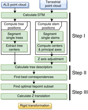
The input data for our method consists of a terrestrial and an ALS point cloud. We assume that the ALS points are given in a geo-referenced coordinate system. No restrictions are made regard-ing the presence or absence of radiometric data (intensity, pulse width) or the return type of the laser scanner (discrete return vs. full waveform). Regarding the terrestrial point cloud, a local co-ordinate system is assumed with arbitrary 3D rotations and trans-lation w.r.t. the ALS CS, but the true object scale must be main-tained. In practice, this requires that the parameters of the camera used for acquiring the ground photographs (focal length etc.) be known. The key assumption is that sufficiently many common trees are present within both captured scenes, and that both point densities are high enough to allow a reliable extraction of tree crowns (ALS) and stems (terrestrial). The output of our method is the rigid transformation which maps the terrestrial CS to that of the ALS point cloud. The processing pipeline describing our approach is depicted in Figure 1. The method consists of three
Figure 1: Overview of coregistration pipeline.
main steps. In the first step, approximate tree positions (intersec-tions of the stem center and the ground) are detected in both input point clouds. For ALS data, this is done on the basis of individ-ual tree clusters, since usindivid-ually no stem hits are available. On the other hand, for the terrestrial data the tree stems are visible at the ground level, and the considerably higher point density enables direct stem detection within the point cloud. First, the points are segmented to form putative stem candidates. For each candidate, we determine its principal direction (axis). The median axis of all candidates is then aligned with theZ axis of the ALS CS. This is an important part of our method, since in later steps we use planimetric and vertical distances between trees. Comparing these distances across the two datasets only makes sense if they are calculated w.r.t. the same reference plane, defined by the CS’s
align the Z axis with the dominant normal vector direction, while we utilize the application-specific tree stem orientation. In the second step of our method, the calculated tree positions are used to form a descriptor for every stem in each dataset. We define a similarity measure on the space of descriptor pairs. The pair-wise similarities are used to set up an instance of the maximum weight matching problem, whose solution yields the set of corre-sponding ALS and terrestrial tree positions. The third step uses the corresponding tree positions as tiepoints for calculating the CS transform which defines the remaining in-plane rotation an-gle and the 2D offset. At this stage, the set of all corresponding tree pairs obtained from the previous step may contain outliers (erroneously matched trees). The goal is to find a maximum tie-point subset which is free from invalid matches. Finally, once the true tiepoint subset is known, the vertical shift is determined, thus completing the CS transformation.
3 TREE POSITION DETECTION
In this section, we explain the details of our approach for cal-culating the tree positions based on the input point clouds. For ALS point clouds, we first calculate the DTM, followed by a 3D segmentation of individual trees (Reitberger et al., 2009). We then approximate the tree center as the 2D location(xc, yc)of the highest point within each segmented tree cluster. We assume the tree axis is parallel to the CSZaxis and so the ground inter-section point’s planimetric coordinates coincide with those of the tree top. The final tree positions are augmented with the DTM heights calculated at each tree center(xc, yc). In the remainder of this section, we focus on the workflow for the terrestrial data.
3.1 Preprocessing
Since we assume that the local CS of the data has an arbitrary rotation, the point cloud may appear inverted, i.e. the ground points will be above the stem points. This is not acceptable since it interferes with parts of the method which rely on the notions of ’up’ and ’down’. We compensate for this by rotating the point cloud (through PCA) so that the ground points appear to lie on theXY plane. The DTM of the point cloud is then calculated using an Active Shape Model formulation (Polewski et al., 2015) and all points within a threshold distancedDT Mof the DTM are removed to filter out ground vegetation. The point cloud is subse-quently voxelized with a width ofdvox. We found this step bene-ficial due to the large amount of noise present in the photogram-metric point cloud, which contains not only points lying ideally on the stem surfaces, but rather a thick, volumetric ring which dis-torts neighborhood calculation (Figure 2(a)). We proceed by ap-plying connected component segmentation with a thresholddcc on the maximum distance between neighboring points. The re-sulting connected components are considered stem candidates. The candidate set is filtered using a minimum point countnccand a minimum dimensionhccto remove objects which are not likely to represent stems. Note that the stem candidates may possess side branches (Figure 2(b),2(c)). Usually, one connected compo-nent corresponds to one tree, but a many-to-one relationship is allowed as the optimal subset of tree locations actually used for defining the transformation is determined in a later step.
3.2 Principal direction calculation
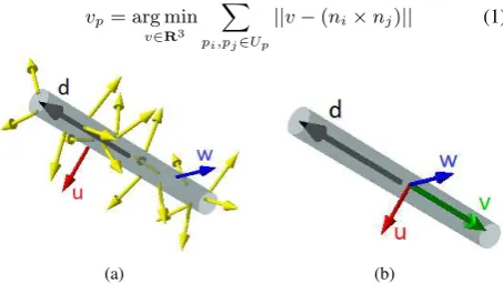
We introduce a method for estimating the principal direction of a cylindrical shape. The approach is designed to be robust in the presence of multiple side branches and point cloud noise. First, surface normals are calculated using local plane fitting. Next, the spherical neighborhoodUpof each pointpis considered. For
(a) (b) (c)
Figure 2: Photogrammetric point clouds of single stems with side branches: (a) top view, (b)-(c) side view.
each point pair(pi, pj), we compute the cross-product between their associated normals, therefore obtaining a new vectorvi,j which is perpendicular to both of the normals. Observe that on a cylindrical surface, the cross-product of two normals (exclud-ing parallel and antiparallel pairs) is collinear with the cylinder’s axis direction (Figure 3). Therefore, ifplies on an approximately cylindrical surface, the dominating direction in the set of vi,j withinp’s neighborhood should represent the principal direction. We formalize this intuition by defining the principal directionv
as the spatial median of the cross-products:
vp= arg min v∈R3
X
pi,pj∈Up
||v−(ni×nj)|| (1)
(a) (b)
Figure 3: (a) Cylinder with directiondand surface normals. (b) The cross productvof normalsu, wis collinear withd.
The spatial median is one of several possible multivariate gener-alizations of the standard (univariate) median. K¨arkk¨ainen and
¨
cylinder axes and not on normals. Also, in the former, a fixed KDE bandwidth is employed, whereas in our approach the KDE bandwidth is estimated in a data-driven manner using the method of Wand and Jones (1994). To find the maximum mode of the un-derlying distribution, we samplektimes from the KDE and pick the maximum-probability sample as the starting point. Gradient ascent is subsequently applied to locate the peak of the corre-sponding mode. The vector associated with the highest probabil-ity is returned as the entire object’s principal direction. The pro-posed method shares some ideas with the Hough-transform based approach of Rabbani and van den Heuvel (2005), where normal vectors from the point cloud vote for the cylinder axis on a Gaus-sian sphere. However, our approach has the advantage that the axis parameter space does not need to be discretized; nor do we need to generate samples to populate the Hough space. Instead, we rely on established statistical methods to determine the KDE kernel bandwidth and perform the search in continuous space.
3.3 Cylinder fitting
Once the cylinder principal direction is determined, we calcu-late the center position and radius based on a sample consensus method. For a cylinder with an axis parallel to one of the coor-dinate axes, 3 point samples are require to uniquely identify the remaining parameters (Beder and F¨orstner, 2006). To exploit this, we rotate the candidate stem point cloud to align the calculated principal direction with theZaxis. We then randomly pick point triplets(Xi, Yi)i=1..3and solve the linear equation system:
2X1 2Y1 −1
2X2 2Y2 −1
2X3 2Y3 −1
t u v
=
X12+Y12 X22+Y22 X2
3+Y32
(2)
w.r.t. the variablest, u, v. The cylinder center is given by(t, u), while the radiusris expressed by:r=√t2+u2−v.
Follow-ing the RANSAC principle, we pick the cylinder parameters re-sulting in the greatest number of inlier points within a prescribed thresholdδ. As a final step, we rotate the obtained center back to the original coordinate system and find the intersection of the now completely characterized cylinder with the DTM. The inter-section point is the putative detected tree location.
3.4 Z axis adjustment
As explained in Section 2, the reference planes for calculating tree heights and positions must be equalized within the terrestrial and ALS point clouds if any planimetric and vertical distance comparisons are to be meaningful. To achieve this, we make use of tree gravitropism and assume that the principal direction shared by most of the trees corresponds to the WorldZaxis. We therefore calculate the spatial median of all candidate stems and align this direction with theZaxis. This boils down to a rotation of the putative tree locations from the previous step. We subse-quently filter out candidate stems whose principal axis angular deviation w.r.t. the median axis is above a thresholdαz= 5◦.
4 COREGISTRATION
After applying the methods outlined in the previous section, the
Z axes of the coordinate systems describing the terrestrial and ALS tree positions are parallel. This leaves the in-plane rota-tion angle, the planimetric offset as well as the vertical shift to be determined. This section explains the details of our proposed approach for calculating these parameters.
4.1 Stem descriptor
We introduce a tree stem descriptor which characterizes the spa-tial relationship of a stem to other trees within the same plot. The
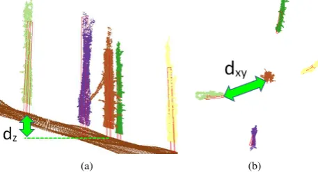
descriptors will then be used to find trees with similar proper-ties across different plots. For each tree stem, the descriptor is constructed through forming a list of pairsDi = (di,xy;di,z) of planimetric as well as vertical distances to the remaining trees (Figure 4). The list is then sorted in an ascending order based on the planimetric distance. We make use of the aforementioned as-sumptions about parallelZaxes of the tree position CSs. Thus, the descriptor is invariant to rotations about theZ axis and ar-bitrary translations. We chose to split the tree position distances into a vertical and 2D component in the hope of increasing dis-criminative capacity compared to the 3D distance. In this way, we can incorporate DTM variability information into the descriptor.
4.2 Similarity measure
Our notion of stem descriptor similarity is based on radial basis functionsKsuch thatK(x, y) =K(||x−y||). In the following, we will refer to them askernels. We begin by defining partial similaritysbetween two distance pairsDi = (di,xy;di,z)and
Dj= (dj,xy;dj,z):
s(Di, Dj) =K(||
di,xy−dj,xy||
hxy
)K(||di,z−dj,z|| hz
) (3)
The structure of the similarity function matches the descriptor’s structure by factoring into two components corresponding to the difference in planimetric and vertical distances between the com-pared pairs. The kernelKis the same for both components, but the bandwidthshxy, hzfor, respectively, the planimetric and ver-tical component are independent. Recalling that our stem de-scriptors are ordered lists of distance pairs, we now define the complete similaritySbetween two descriptorsF = (Fi)i=1..m andG= (Gj)j=1..n:
(a) (b)
Figure 4: Tree stems on DTM with marked stem descriptor dis-tances. (a) side view -Zdistance, (b) top view -XY distance.
S(F, G) =T(m, n)
T(i, j) = max
T(i−1, j−1) +s(Fi, Gj)
T(i−1, j) +pg
T(i, j−1) +pg
T(i−2, j−2) +s(Fi−1, Gj) +s(Fi, Gj−1)
The formulation given above is based on the algorithm by Needle-man and Wunsch (1970) for aligning DNA sequences. The algo-rithm finds the optimal (maximum-similarity) alignment between the input sequences by recursively solving the problem on shorter subsequences and combining the smaller problem’s solution with the elements as the currently processed position. In each move
(i, j), 4 options are considered: (i) matchFiwithGj, combine with best match ofF1..i−1 andG1..j−1, (ii) matchFiwith gap, combine with best match of F1..i−1 andG1..j, (iii) matchGj with gap, combine with best match ofF1..i andG1..j−1, (iv)
match ofF1..i−2andG1..j−2. The gap penaltypgis not signifi-cant in our setting (pg = 0). The total matching score is defined as the score of the full-length sequencesF1..mandG1..n. Note that by splitting the tree distance into two components, we in-creased discriminative power at the cost of the ability to uniquely sort the descriptor elements (due to 2 dimensions). Therefore, the sorted sequence-based matching is an approximation of the opti-mal matching without ordering. On the other hand, computing this exact matching requires graph based methods whose com-putational complexity ofO(max(m, n)3)far exceeds that of the
Needleman-Wunsch algorithm (O(m∗n)). This makes the exact method impracticable even for moderate datasets (100-200 trees).
4.3 Graph matching
We compute the descriptor similarityS between all pairs of de-scriptorsFa, Gb
such that theFa
correspond tomtrees from the terrestrial dataset, whileGbrepresentntree positions from the ALS point cloud. We define a bipartite graphG= ((V1, V2), E), whereE ⊆ V1 ×V2, such thatV1 andV2are respectively the set of descriptorsFaandGb. The graph’s weighting function
w : E → R is then defined asw(a, b) = S(Fa, Gb). We
then find a maximum weight matching using the standard Kuhn-Munkres method, known in literature as the Hungarian algorithm. Note that since in general the number of trees in both plots may differ, onlymin(m, n)trees will be matched. These tree posi-tions will be considered as tiepoints in the subsequent steps.
4.4 Rigid transformation
For two fixed, equal length listsP1, P2of corresponding plani-metric tree positions, the 2D rigid transformation which alignsP1
toP2may be computed using algorithm due to Kabsch (1976). First, the centroidsc1, c2are determined, followed by the covari-ance matrixBbetween the (centered) tree positions. LetV SWT be the singular value decomposition ofB. Then, the optimal (least-squares) rotationRand translationtxyare given by:
R=W VT, txy=−Rc1+c2
4.5 Determination of tiepoint subset
As a result of the graph matching procedure, all trees within the smaller of the two datasets (terrestrial, ALS) will be matched. However, it is expected that a considerable part of the correspond-ing pairsCwill be invalid, because some of the trees simply do not have true matches in the other dataset. Therefore, it is neces-sary to find a subset of true correspondences that will determine the final CS transformation. While for a small number of tiepoint candidates (trees in the plot) all2min(m,n) subsets may be
ex-amined, this approach is computationally intractable in the gen-eral case because of the exponential computational complexity. We propose a heuristic algorithm which iteratively augments the current best set of tiepoints by exploring the solution’s neighbor-hood, starting from a small initial solution (k0tiepoints) obtained from exhaustive search. The algorithm is given in Listing 1. The
error(T)function represents the average deviation between the matched tiepoints in setT ⊆Cobtained after applying the trans-formation calculated as described in Section 4.4. The function
matchedInRange(T, C, r)calculates the transformation onTand returns all correspondences fromC\Twhose distance between the matched points is belowr. The algorithm can be viewed as a hybrid between exhaustive search and a greedy strategy, with the parameterτcontrolling the maximum size of the tiepoint subset which gets replaced during the search. A value ofτ = 1 corre-sponds exactly to greedily picking the tiepoint whose introduc-tion into the best soluintroduc-tionT(i−1)results in the bestT(i). Asτ
Algorithm 1Finding optimal tiepoint subset
1: functionBESTTIEPOINTSUBSET(C,k,τ)
2: T(k0)←exhaustiveSearch(C, k0, τ) 3: fori=k0+ 1..kdo
4: forj= 1..min(τ, i−k0)do
5: Cr ←matchedInRange(T(i−j), C, dthr)
6: Tj
i ←arg minD⊆Cr,|D|=jerror(T(i−j)∪D)
7: T(i)← Tj′
i , j
′←arg min jerror(T
j i)
8: return(T(k0), . . . ,T(k))
is increased, the computational effort increases but a larger area of the solution space is visited. The algorithm returns the list of optimal tiepoint subsets for each processedkvalue. Note that due to the thresholddthr, only matches whose points lie reasonably close are considered as tiepoint candidates, so the algorithm may terminate prematurely if no more candidates compatible with the current best transform are found.
4.6 Vertical offset calculation
In the final step, the optimal vertical offset is determined on the set of tiepointsTobtained from the previous phase of the coregis-tration as the median of signed deviationszALS
i −z terr i between ALS and terrestrial tiepoint heights.
5 EXPERIMENTS
5.1 Data acquisition
The study area is located in the northern interior of the Coast Range in western Oregon (45.301502◦N,123.380802◦W). The site has a mean canopy height of 35.9 m and an average height to live crown base of 23.7 m and is characterized by pure silvi-cultural stands of Douglas-fir with vine maple (Acer circinatum Pursh) present in the understory. The plot is situated at 484.3 m elevation with a slope of 23% and dimensions of 76x121 m2.
ALS data The LiDAR data was collected by Quantum Spatial on April 17th, 2011 using a discrete-return Leica ALS60 config-ured to a pulse rate of>105 kHz, at an altitude AGL of 900 m. The processed point cloud had a mean ground density of 0.87 points/m2, and mean pulse density of 10.18 points/m2. The point cloud was segmented into 169 individual trees (Figure 5(a)).
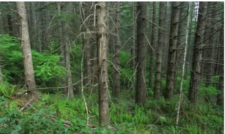
Terrestrial photographs We conducted a ground-level imag-ing survey on May 5th, 2014 usimag-ing a Canon PowerShot S100 digital compact camera with a focal length of 5.2 mm. We col-lected a total of 443 images at a mean altitude AGL of 1 m, cov-ering a calculated area of 2747 m2at a ground surface resolution of 8.7 mm/pixel, with 1 pixel of error and a point density of 3305 points/m2. See Figure 6 for an example terrestrial image.
Initial data processing To compute the photogrammetric point cloud, we first filtered out images of poor quality due to motion and out-of-focus blurring. We then carried out structure-from motion (SfM) dense reconstruction using Agisoft Photoscan Pro-fessional, whose processing pipeline consists of a proprietary im-plementation of the scale-invariant feature transform (SIFT), a bundle adjustment, and a dense matching algorithm. The result-ing point cloud is depicted in Figure 5(b).
5.2 Scenario simulation
(a) (b)
Figure 5: Target area - (a) ALS point cloud (color by single trees), (b) terrestrial point cloud (RGB)
Figure 6: Sample ground-level photograph of target plot
site. The simulation starts by generatingm3D stem positions, wheremequals tree count in the ALS dataset. Thez coordi-nate is taken as the ALS DTM height at the 2D position, while the planimetric tree locations are created on the basis of a ker-nel density estimation model of the 2 nearest neighbor (2NN) distances between trees in the ALS point cloud (obtained using manually marked tree positions). This way, the distributions of the distances to the two nearest neighboring trees are approxi-mately equal in the real and simulated data (15% tolerance). We then pick a randomly-oriented rectangle containing a subset of the generated locations, with dimensions equal to those of the terrestrial point cloud, which will represent the artificial terres-trial scenario. To account for the fact that not all trees captured by ALS are also present in the terrestrial dataset, we randomly re-move a percentage of the created ALS tree positions. Then, more locations are generated according to the KDE of the terrestrial point cloud’s 2NN distribution so that the total number of trees within the picked rectangle approachesn(tree count in the real terrestrial data). As a result, we obtain two associated sets ofm
andn3D tree positions which can be used as validation data after adding the required amount of noise. Note that the simulated sce-narios are related to the real data through both the 2NN distance distribution, and thezdistribution from the real DTM.
5.3 Reference data and evaluation criterion
We utilized two quality measures: (i) quality of found matches, computed as the ratio of point pairs correctly matched by our method to the actually matching point pair count, and (ii) mean planimetric distance of matched points after transformation (sep-arately on tiepoints only and on all matching points). For the simulated data, all correspondences, true tree positions etc. were known by construction. For the real data, we did not have access to field measurements of ground-truth tree positions. Therefore, we manually marked the tree tops (ALS) and stem positions (ter-restrial) in both datasets based on visual inspection, resulting in 169 tree locations in the former and 59 in the latter. Our sub-jective estimate of the positioning error w.r.t. true tree locations
is 0.7 m (ALS) and 0.35 m (terrestrial). We then constructed a list of 32 matching tree pairs which were present in both datasets using initial coregistration results. The mean matched point dis-tance for the real dataset was calculated w.r.t. these 32 pairs. The automatic stem detection routine (Section 3) found 44 of the 59 trees in the ground dataset, out of which 24 were manually linked with an ALS tree position. Note that due to lack of stem points as well as overstory cover and general structure of the ALS point cloud, it was not possible to obtain an estimate of the correctly detected tree ratio for the ALS dataset. The mean deviations be-tween the manual and automatic tree positions were 0.32 m and 0.46 m respectively for ALS and terrestrial data.
5.4 Parameter settings
The DTM thresholddDT M was 1 m to filter out ground veg-etation. Based on the photogrammetric point cloud density, the voxel width, connected component distance, SAC model distance and min. point count were set todvox= 1cm,dcc=δ= 5cm, andncc = 200. The min. trunk heighthccwas 1.5 m, and the max. tiepoint matching distancedthr= 1m. The Gaussian ker-nel was used in the role of the similarity measureK.
5.5 Detailed experiments
Evaluation on simulated data We carried out experiments on simulated scenarios to determine the dependence of the match quality as well as the mean matched point distance on the amount of noise present in the data. For this purpose, we created sce-narios with additive uniform noise on each 2D input position set having mean values of 5 to 75 cm, with sizes matching the real data: 170 and 60 locations respectively in the simulated ALS and terrestrial dataset, and about 30 trees occurring in both (true cor-respondences). For each noise pair (ALS, terrestrial), 50 sce-narios were evaluated. Two amplitudes of uniformly distributed vertical noise were tested: 0-1 m and 0-0.5 m. All experiments were done in 3 configurations of the similarity measure (Eq. 3): split 2D-vertical, uniform 3D (single 3D distance), only 2D.
Evaluation on real data First, we investigated the influence of the tiepoint set size on the matching distance. This was done by randomly sampling subsets of the true correspondences starting at 3 tiepoints (up to the maximum number of matched points), calculating the CS transformation based on the subset and record-ing the mean matched point distance. For each tiepoint set size, the results are averaged over 200 random samplings. The second experiment corresponded to an application of our method in a real-world scenario, where no prior knowledge (amount of noise, true correspondences) is available. We executed the full pipeline of calculating the tree matching and finding the optimal tiepoint subset (Section 4), through a grid search on the kernel bandwidths
hxy, hz on a range of 0.1 to 1.5 m. As the result of the grid search, we picked the kernel configuration which led to the maxi-mum number of matched tiepoints (Algorithm 1). We performed this both for the set of tree positions from manual labeling and the automatically detected positions (Section 3).
6 RESULTS AND DISCUSSION
Simulated data
m, whereas this threshold rises to 0.65 m and 1 m in case of the split distance for vertical noise meanµzequal to respectively 0.25 m and 0.5 m. These differences are even more pronounced in Fig-ure 7(b), which depicts the mean distance between the true corre-sponding points after coregistration. For the 2D and 3D distance, the coregistration fails when one of the noise means exceeds 0.15 m. The failure is a consequence of poor point matching, which in turn leads to the coordinate transformation being based on wrong correspondences and results in matching distances exceeding 20 m. On the other hand, the split distance (2D+Z) exhibits stable re-sults whenmax(µ1, µ2)is below 0.45 m and 0.65 m for the two respectiveµzvalues, with mean matched point distances usually within the interval[(µ1+µ2)/2; max(µ1, µ2)].
Tree position matching quality - simulated data 2D+Z(µz=0.25m)
Mean matched tree position distances [m] - simulated data 2D+Z(µz=0.25m)
Figure 7: Results for simulated data as a function of tree posi-tion noise means: (a) avg. correctly matched point ratio, (b) avg. matched point distance [m].µzindicates vertical noise mean.
Real data
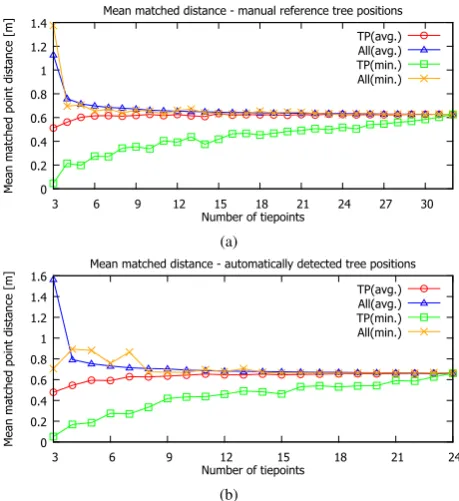
We now turn to the real data obtained through ALS and pho-togrammetric techniques (Section 5.1). In the second experiment, we examined the influence of the number of tiepoints used to cal-culate the coordinate transformation on the final matched point distance. For this purpose, we used correspondences between the ALS and terrestrial tree positions that were manually deter-mined through visual inspection. Two such correspondence sets were derived, one for the reference tree positions marked manu-ally, and the other for the automatically detected tree positions. In case of the reference positions (Figure 8(a)), we observe that on average (blue△curve), the mean matched distance over all 32 corresponding tree positions based on 3 tiepoints (TP) is not satisfactory, exceeding 1.1 m, whereas at 6 TP, the distance drops below 0.7 m and declines steadily to reach 0.63 cm at 20 TP. In contrast to the matched distance averaged over multiple runs, the orange (x) curve shows the result taken for the single tiepoint set whose mean inter-TP distance was minimal among all runs. It is interesting to note that result of 1.4 m for 3 TP is worse than average 1.1 m, which indicates that the mean matched dis-tance over tiepoints only is not always correlated with the mean matched distance over all points. For the automatically detected positions (Figure 8(b)), the average (△) trend is similar, while the min (x) curve behaves somewhat differently. For 3 TP, a good
result (0.71 m) is achieved, but in the range of 4-8 TP, random fluctuations appear, with the mean distance deteriorating to 0.88 m and then returning below 0.7 m. The trend fully settles for 15 TP, after which point it becomes indistinguishable from the average curve. We conclude that it may be worthwhile to con-duct the coregistration using 10-15 TP, since in the real scenario the true correspondences are unknown and only the mean TP dis-tance guides the coregistration process. The last experiment
0
Mean matched distance - manual reference tree positions
TP(avg.)
Mean matched distance - automatically detected tree positions
TP(avg.) All(avg.) TP(min.) All(min.)
(b)
Figure 8: Mean coregistration distance on tiepoints (TP) and all matched points (All) for real data when true correspondences are known, by tiepoint set size
uates the real-world application with no prior knowledge of cor-respondences. The final mean matched distances of the set of all matched points (all) and tiepoints only (TP) are depicted in Fig-ure 9. We conducted the grid search on kernel bandwidths as de-scribed in Section 5.5 and picked the kernel pair which resulted in the most tiepoint pairs matched by Algorithm 1. This can be seen as an objective, unsupervised measure of matching quality, since a large number of matching pairs is unlikely to arise randomly. For the two-part kernel (2D+Z), a total of 17 and 18 matching TP were found respectively for the manual reference and auto-matic tree positions. In case of the uniform distance kernel (3D), for the manual positions a subset of 7 TP was found, while for the automatic positions all configurations failed. This aligns well with the simulation results (Figure7), which essentially predicted a breakdown of the uniform kernel for position deviations ex-ceeding 15 cm. The fact that a 3D kernel solution existed for manual positions suggests that their determination through visual inspection was reasonably precise (at least 7 trees with deviations
cm) and slope of 23%. Finally, although the true accuracies of the stem positions are unknown, we can roughly estimate the noise meansµ1, µ2by finding the point on the simulated matched dis-tance surface (Figure 7(b)) which best matches our result of 66 cm. The closest matches were mean values of 0.35 m/0.25 m for
µz = 0.25m and 0.4 m/0.25 m forµz = 0.5m. The coregistered tree planimetric positions obtained via our method on the test plot are shown in Figure 10.
0
Mean matched distance for best kernel bandwidths
2D + Z: TP(ref.) 2D + Z: All(ref.) 3D: All(ref.) 2D + Z: TP(det.) 2D + Z: All(det.)
Figure 9: Results of kernel bandwidth grid search for real data -mean matched point distance curves by tiepoint count for manual reference (ref.) and automatically detected (det.) positions
0
Figure 10: Coregistered tree positions on test plot (axes in m).
7 CONCLUSIONS
We presented a method for coregistering ALS and terrestrial pho-togrammetric point clouds in forested areas. The method finds corresponding trees in both point clouds using mutual distances between stem positions within the plot. We showed that incor-porating DTM variability into the distance metric can yield im-proved discriminative capabilities compared to a purely planimet-ric variation, which leads to enhanced quality of the tree match-ing. Evaluations on real and simulated data indicate that a good correspondence quality (average planimetric distance of 66 cm between matched tree centers) may be achieved, considering the limited accuracy of tree center detection for ALS data. This agreement between terrestrial and ALS tree distances confirms that the real-world scale assumption for the photogrammetric point cloud is valid in practice. Furthermore, the proposed simulation procedure is tailored to the target area’s properties (inter-tree dis-tances, DTM shape), and therefore may be used to assess the suit-ability and expected accuracy of our method for a particular new area. Our results could be a step towards a new generation of cheap systems for surveying the forest understory based on hand-held terrestrial photogrammetry. As a future step, we would like to increase the tree center calculation accuracy particularly for the ALS data, as it is currently the dominating error source. Also, precise field measurements could provide a basis for better quan-tifying the coregistration error.
REFERENCES
Amiri, N., Yao, W., Heurich, M. and Krzystek, P., 2015. Regen-eration detection by 3D segmentation in a temperate forest using airborne full waveform lidar data. In: Proceedings of SilviLaser.
Beder, C. and F¨orstner, W., 2006. Direct solutions for computing cylinders from minimal sets of 3d points. In: Proceedings of the 9th European Conference on Computer Vision - Volume Part I, ECCV’06, Springer-Verlag, Berlin, Heidelberg, pp. 135–146. Gupta, V., Reinke, K. J., Jones, S. D., Wallace, L. and Holden, L., 2015. Assessing metrics for estimating fire induced change in the forest understorey structure using terrestrial laser scanning. Remote Sensing 7(6), pp. 8180–8201.
Hauglin, M., Lien, V., Naesset, E. and Gobakken, T., 2014. Geo-referencing forest field plots by co-registration of terrestrial and airborne laser scanning data. Int. J. Remote Sens. 35(9), pp. 3135–3149.
Hyypp¨a, J., Holopainen, M. and Olsson, H., 2012. Laser scanning in forests. Remote Sensing 4(10), pp. 2919–2922.
Kabsch, W., 1976. A solution for the best rotation to relate two sets of vectors. Acta Crystallographica A 32, pp. 922–923.
K¨arkk¨ainen, T. and ¨Ayr¨am¨o, S., 2005. On computation of spa-tial median for robust data mining. In: R. Schilling, W. Haase, J. Periaux, H. Baier and G. Bugeda (eds), Evolutionary and De-terministic Methods for Design, Optimization and Control with Applications to Industrial and Societal Problems.
Kelbe, D., 2015. Forest structure from terrestrial laser scanning in support of remote sensing calibration/validation and opera-tional inventory. PhD thesis, Rochester Institute of Technology. Korpela, I., Hovi, A. and Morsdorf, F., 2012. Understory trees in airborne lidar data selective mapping due to transmission losses and echo-triggering mechanisms. Remote Sens. Environ. 119. Lindberg, E., Holmgren, J., Olofsson, K. and Olsson, H., 2012. Estimation of stem attributes using a combination of terrestrial and airborne laser scanning. Eur. J. Forest Res. 131(6).
Needleman, S. B. and Wunsch, C. D., 1970. A general method applicable to the search for similarities in the amino acid se-quence of two proteins. Journal of Molecular Biology 48(3), pp. 443 – 453.
Novak, D. and Schindler, K., 2013. Approximate registration of point clouds with large scale differences. ISPRS Annals of Pho-togrammetry, Remote Sensing and Spatial Information Sciences II-5/W2, pp. 211–216.
Polewski, P., Yao, W., Heurich, M., Krzystek, P. and Stilla, U., 2015. Detection of fallen trees in ALS point clouds using a Normalized Cut approach trained by simulation. ISPRS J. Pho-togramm. Remote Sens. 105, pp. 252 – 271.
Rabbani, T. and van den Heuvel, F., 2005. Efficient hough trans-form for automatic detection of cylinders in point clouds. In: IAPRS, XXXVI, 3/W19, pp. 60–65.
Reitberger, J., Schn¨orr, C., Krzystek, P. and Stilla, U., 2009. 3D segmentation of single trees exploiting full waveform LIDAR data. ISPRS J. Photogramm. Remote Sens. 64(6), pp. 561 – 574. St-Onge, B., Audet, F.-A. and B´egin, J., 2015. Characterizing the height structure and composition of a boreal forest using an individual tree crown approach applied to photogrammetric point clouds. Forests 6(11), pp. 3899.
Theiler, P. W., Wegner, J. D. and Schindler, K., 2014. Keypoint-based 4-points congruent sets automated marker-less registration of laser scans. ISPRS J. Photogramm. Remote Sens. 96, pp. 149. Wand, M. P. and Jones, C., 1994. Multivariate plug-in bandwidth selection. Computational Statistics 9(2), pp. 97–116.
Weinmann, M. and Jutzi, B., 2015. Geometric point quality as-sessment for the automated, markerless and robust registration of unordered TLS point clouds. ISPRS Annals of Photogramme-try, Remote Sensing and Spatial Information Sciences II-3/W5, pp. 89–96.