23 11
Article 06.3.4
Journal of Integer Sequences, Vol. 9 (2006),
2 3 6 1
47
On the Farey Fractions with Denominators in
Arithmetic Progression
C. Cobeli
1and A. Zaharescu
2Institute of Mathematics of the Romanian Academy
P. O. Box 1-764
Bucharest 70700
Romania
Abstract
Let FQ be the set of Farey fractions of order Q. Given the integers d ≥ 2 and 0≤c≤d−1, letFQ(c,d) be the subset of FQ of those fractions whose denominators are≡c (modd), arranged in ascending order. The problem we address here is to show that asQ→ ∞, there exists a limit probability measuring the distribution ofs-tuples of consecutive denominators of fractions inFQ(c,d). This shows that the clusters of points (q0/Q, q1/Q, . . . , qs/Q)∈[0,1]s+1, whereq0, q1, . . . , qs are consecutive denominators of
members of FQ produce a limit set, denoted by D(c,d). The shape and the structure of this set are presented in several particular cases.
1
Introduction
Farey fractions have many applications in various areas of mathematics. Recently, they have been successfuly used in some problems on billiards [3, 4] and the two dimensional Lorentz gas [5]. The present paper is a continuation of a series of papers dedicated to the study of the distribution of neighbor denominators of Farey fractions whose denominators are in arithmetic progression. Previously [10, 11, 13, 14] different authors have treated the cases of pairs of odd and even denominators, respectively, while here we deal with tuples of consecutive denominators of fractions in FQ(c,d), the set of Farey fractions with
1
C. Cobeli is partially supported by the CERES Programme of the Romanian Ministry of Education and Research, contract 4-147/2004.
2
denominators ≡ c (mod d). (Here c,d are integers, with d ≥ 2 and 0 ≤ c ≤ d−1.) The motivation for their study [1, 3, 4, 6, 7, 8, 9] comes from their role played in different problems of various complexities, varying from applications in the theory of billiards to questions concerned with the zeros of Dirichlet L-functions. Although the present work is mostly self-contained, the reader may refer to the authors [11] and the references within for a wider introduction of the context and the treatment of some calculations.
Two generic neighbor fractions from FQ, the set of Farey fractions of order Q, say a′/q′
and a′′/q′′, have two intrinsic properties. Firstly, the sum q′+q′′ is always greater than Q
and secondly, a′′q′−a′q′′ = 1. None of these two properties is generally true for consecutive
members ofFQ(c,d), but we shall see that they may be recovered as initial instances of some more complex connections.
Given a positive integer s ≥ 1, our main interest lies on the set of tuples of neighbor denominators of fractions in FQ(c,d):
DsQ(c,d) := ½
(q0, q1, . . . , qs) : q
0, q1, . . . , qs are denominators of
consecutive fractions in FQ(c,d) ¾
.
(Notice that due to some technical constraints, in our notations, the dimension is s+ 1 and not s.) In fact our aim is to show that there is a limiting set Ds(c,d) of the scaled set of
points DQ
s(c,d)/Q⊂[0,1]s+1, as Q→ ∞. Strictly speaking, this is the set of limit points of
sequences {xQ}Q≥2, where each xQ is picked from DsQ(c,d)/Q.
More in depth information onDs(c,d) is revealed if one knows the concentration of points
across its expanse. The answer is given by Theorem 2 below, which shows that there exists a local density function on Ds(c,d) and gives an explicit expression for it. Next, let us
see the formal definition. Let x= (x0, . . . , xs) be a generic point in [0,1]s+1 and denote by
gs(x) =gs(x;c,d) the function that gives the local density of points (q0/Q, q1/Q, . . . , qs/Q) in
thes+1-dimensional unit cube, asQ→ ∞, whereq0, q1, . . . , qsare consecutive denominators
of fractions in FQ(c,d). At any pointu = (u0, . . . , us)∈[0,1]s+1, we define gs(u) by
gs(u) := lim η→0
lim
Q→∞
#¡✷∩DQs(c,d)/Q¢
#DQs(c,d)
4η2 , (1)
where ✷⊂Rs+1 are cubes of edge 2η centered at u.
The fact that any sequence of consecutive denominators in FQ is uniquely determined by its first two terms has important consequences. Here we are interested in the shape of
Ds(c,d). It turns out that the framework of Ds(c,d) is built by a union of two dimensional
compact surfaces in Rs+1. This is the reason for which we have divided in the right-hand
side of (1) by the area of a square of edge 2η only, and not by (2η)s+1.
Thus, basically, gs(u) = gs(u, v) is a function of two variables. Here (u, v) will run over a
domain that embodies the Farey series, namely the Farey triangle with vertices (0,1); (1,0); (1,1), denoted by T.
The first thing to be remarked is the fact that for anyd≥2,D1(c,d) is a polygon obtained as a union of some sequences of polygonal sets with constant local density on each of them. Moreover, one of these polygons is large enough to include all the others. But the most noteworthy property is that each of these constant-density-polygons has a vertex at (1,1) and looks like a mosaic composed by polygonal pieces, most of them being quadrangles. The fact that the mosaics exist is not just an accidental occurrence; on the contrary, more and more pieces fit into mosaics with a larger and larger number of components as d increases. The mosaics are either symmetric with respect to the first diagonal or they appear in pairs, whose components are symmetric to each other with respect to the first diagonal.
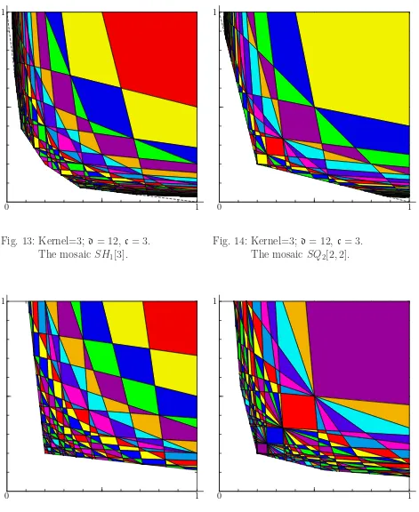
It is not true, as one would guess from tests with many acceptably smalld’s and different c’s, that the larger mosaic (most likely equal to D1(c,d)) is always a quadrangle. The first counter-example is D1(3,12), which is a hexagon (see Fig. 13). The shape of the mosaics is more regular when d has fewer prime factors. In particular, for each prime modulus d, the exterior frame of all the mosaics is the same with that from the case d = 2, c = 0 (cf. [11, Fig. 5, 6]), which in turn was the same in the case d = 2, c = 1 (cf. [10, Fig. 2]). Mosaics having exactly the same form appear in other cases, too. For example, this happens when d= 4, c= 0, and the event has another interesting feature: each of the mentioned mosaics appear twice. As opposed to the prime modulus instance, we have included in Section 11
the pictures that appear in the case d = 12, c = 3. One may appreciate these mosaics for their proportions, unexpected shape and beauty.
2
Notations and Prerequisites
Suppose the integer Q is sufficiently large, but fixed. We also fix d ≥ 2, the modulus, 0≤c≤d−1, the residue class, and an integer s ≥1 (s+ 1 is the dimension).
Then, we define recursively the following objects. For 0 < x, y ≤1, let xL
j(x, y) =xLj be
given byxL
−1 =x,xL0 =yand xLj =kjxLj−1−xLj−2, forj ≥1, wherekj =kj(x, y) :=
h1+xL j−2
xL j−1
i . We say that x, y are generators of xL, and of k also, or that xL and k are generated by
x, y. (We use bold fonts to denote vectors with components indicated by the same letters in normal font and subscripts belonging to ranges that become clear from the context.)
In order to get a sequence of consecutive denominators of fractions in FQ, it suffices to know only the first two of them. Moreover, any two coprime integers 1 ≤ q′, q′′ ≤ Q, with
q′ +q′′ > Q, appear exactly once in the sequence of consecutive denominators of fractions
in FQ. Then the subsequent denominators are obtained as follows. Given two neighbor denominators 1 ≤ q′, q′′ ≤ Q, they are succeeded by qL
1, qL2, . . ., where qjL(q′, q′′) = qLj :=
kjqjL−1 −qLj−2, for j ≥ 1, and kj = kj(q′, q′′) =
hQ+qL j−2
qL j−1
i
. We put qL
−1 = q′, qL0 =q′′. Notice that these values of kj coincide with those defined above if x =q′/Q and y= q′′/Q. Then,
in order to simplify the notation, we write k(q′, q′′) instead of k(q′/Q, q′′/Q). As before, we
say thatq′, q′′ are generators of qL and of kor that qL and k are generatedby q′, q′′.
A good way to look at a tuple k= (k1, . . . , kn) is to think that it is associated with the
whole (n+2)-tupleq= (q′, q′′, q
1, . . . , qn) of consecutive denominators inFQ. We remark that
k3 = (q1 +q3)/q2,k4 = (q2+q4)/q3, etc.
It is plain that kj ≥1 for j ≥1. In the extreme case n= 0, the vector kis empty (that
is, it has no components) because there is no mediant between consecutive denominators. In this case we say that khas order zero.
In general, consecutive fractions in FQ(c,d) are not necessarily consecutive in FQ, but have intercalated in-between several other fractions from FQ. We remark also that many consecutive denominators of fractions in FQ(c,d) are not necessarily coprime. Let r = (r1, . . . , rs) be an s-tuple of positive integers, and denote |r| = r1 +· · ·+rs. We say that
q= (q0, . . . , qs), a tuple of consecutive denominators of fractions inFQ(c,d), is of type T(r),
if q ≡ c (modd)3 and there exists a pair of consecutive denominators (q′, q′′) in FQ with
qL
−1(q′, q′′) = q0, q−L1+r1(q
′, q′′) = q
1, . . . , q−L1+r1+···+rs(q
′, q′′) = q
s, andqjL(q′, q′′)6≡ c (modd),
for j ∈ ©
0, . . . ,|r| −1ª
\©
r1−1, . . . , r1+· · ·+rs −1
ª
. In this case we also say that the tuple k(q′, q′′;|r| −1) = (k
1, . . . , k|r|−1), with kj = kj(q′, q′′) is of type T(r). To select the
components that are ≡c (modd), we define the choice application FQ
r : N2 →Ns+1, with
FrQ(q′, q′′) :=¡
q−L1, q−L1+r1, . . . , q
L
−1+r1+···+rs ¢
.
Similarly, for x, y ∈(0,1], with x+y >1, we also put
Fr(x, y) :=
¡
xL−1, xL−1+r1, . . . , x
L
−1+r1+···+rs ¢
.
Let Ar(c,d) be the set of all k(q′, q′′;|r| −1) of type T(r), for any q′, q′′. We remark
that the generators of such a k are, in general, not unique. Then, for any k∈ Ar(c,d), we
consider the set of residues relatively prime toc, given by
Mk,r(c,d) =
©
1≤e≤d: k(c, e;|r| −1) =kª.
For example, suppose Q = 25, c = 1, d = 5. One can find in F25 the following series of consecutive fractions:
. . . , 7
16, 11 25, 4 9, 9 20, 5 11, 11 24, 6 13, 7 15, 8 17, 9 19, 10 21, . . .
From these only 7/16,5/11,10/21 survive, and are consecutive, in F25(1,5). Then, in our terminology, the tuple of denominators (16,11,21) is of type T(r), with r = (4,6). In particular, we see that r1 −1, . . . , rs−1 are, respectively, the number of denominators of
consecutive fractions in FQ that are 6≡ c (modd) intercalated between the fractions with denominators that are≡c (modd). Also,k(16,25; 9) = (1,5,1,4,1,3,2,2,2)∈ Ar(1,5) has
|r| −1 = 4 + 6−1 = 9 components, and
FrQ(16,25) =¡
16,11,21¢
.
3
Lattice Points in Plane Domains
Given a set Ω ⊂R2 and integers 0≤ a, b <d, let N′
a,b;d(Ω) be the number of lattice points
in Ω with relatively prime coordinates congruent modulo d toa, b, respectively, that is,
Na,b′ ;d(Ω) := #
©
(m, n)∈Ω : m≡a (modd); n≡b (mod d); gcd(m, n) = 1ª
.
3
Notice that when gcd(a, b,d)>1, the set in the definition above is empty, so N′
a,b;d(Ω) = 0.
Lemma 1. Let R > 0 and let Ω⊂R2 be a convex set of diameter ≤R. Let d be a positive integer and let 0≤a, b < d, with gcd(a, b,d) = 1. Then
Na,b′ ;d(Ω) =
6
π2d2 Y
p|d
µ 1− 1
p2 ¶−1
Area(Ω) +O¡
RlogR¢
. (2)
The proof follows by a standard argument, as in the proof of [2, Lemma 3.1].
As a consequence of Lemma 1, we obtain an asymptotic formula for the cardinality of FQ(c,d). For this we use (2) and two more facts. Firstly, the area of the Farey triangle is Area(TQ) = Q2/2 and secondly, #FQ(c,d) is the number of lattice points (a, b)∈ TQ× TQ
with relatively prime coordinates, a ≡ c (mod d), and no other condition on b. Since the number of integers 0≤e <d for which gcd(c, e,d) = 1 isd·ϕ(gcd(c,d))/gcd(c,d), it follows that
#FQ(c,d) = 3Q 2
π2 ·
ϕ(gcd(c,d)) gcd(c,d)d
Y
p|d
µ 1− 1
p2 ¶−1
+O¡
dQlogQ¢
. (3)
4
The Density of Points of type
T
(
r
)
We count separately the contribution to gs(x;c,d) of points of the same type. Thus, we
denote by gr(x) = gr(x;c,d), the local density in the unit cube [0,1]s+1 of the points
(q0/Q, q1/Q, . . . , qs/Q) of type T(r), as Q → ∞. At any point u = (u0, . . . , us) ∈ [0,1]s+1,
this local density gr(u) is defined by
gr(u) := lim η→0
lim
Q→∞
#¡✷∩DQr(c,d)/Q ¢
#DQs(c,d)
4η2 , (4)
where
DQr(c,d) := ½
(q0, q1, . . . , qs) of type T(r) : q
0, q1, . . . , qs are denominators of
consecutive fractions in FQ(c,d) ¾
,
and ✷ ⊂Rs+1 are cubes of edge 2η centered at u. Then, we have gs(u) =
X
r
gr(u), (5)
provided we show that each local density gr(u) exists, as Q→ ∞. In the following we find
each gr(u).
5
The Witness Set
Let η > 0 be small and let x0 = (x0
0, . . . , x0s) ∈ [0,1]s+1 be the point around which we
¤=¤η(x0) = (x00−η, x00+η)× · · · ×(x0s−η, x0s+η). Then, givenr = (r1, . . . , rs), we need
to estimate the cardinality of
BrQ(c,d) = ½
(q′, q′′)∈N2: 1≤q
′, q′′≤Q, gcd(q′, q′′) = 1, q′+q′′ > Q,
k(q′, q′′;|r| −1)∈ Ar(c,d), FrQ(q
′, q′′)∈Q·
✷ ¾
.
This reduces to an area estimate if we put ΩQr(c,d) =
½
(x, y)∈[1, Q]2: x+y > Q,
k(x, y;|r| −1)∈ Ar(c,d), FrQ(x, y)∈Q·✷
¾
.
Then, by Lemma 1, #BrQ(c,d) = X
e∈Mk,r(c,d)
Nc′,e;d
¡
ΩQr(c,d)¢
= 6
π2d2Q 2Y
p|d
µ 1− 1
p2 ¶−1
X
e∈Mk,r(c,d) Area¡
Ωr(c,d)
¢ +O¡
dQlogQ¢
,
(6)
where
Ωr(c,d) =
½
(x, y)∈(0,1]2: x+y >1,
k(x, y;|r| −1)∈ Ar(c,d), Fr(x, y)∈✷
¾
.
For any k, we denote
Tk :=
©
(x, y)∈(0,1]2: x+y >1, k(x, y;|r| −1) =kª
and
Pk(η) :=
©
(x, y)∈(0,1]2: Fr(x, y)∈✷
ª
. (7)
Notice that the dependence onkof the setPk(η) is through the components ofFr(x, y) (see
(11) below). Also, we put T0 :=T, the Farey triangle. Then, we have
Area¡
Ωr(c,d)
¢
= X
k∈Ar(c,d) Area¡
Tk∩ Pk(η)
¢
. (8)
By a compactness argument it follows that only finitely many terms of the series are non-zero, although Ar(c,d) may be infinite. Next we need to see the shape of Pk(η), since
we are mainly interested to know Area¡
Pk(η)
¢
. This is the object of the next section.
6
The index
p
r(
k
)
and the polygon
P
k(
η
)
The integer valueskj defined in Section2 satisfy the classicalmediantproperty of the Farey
series. For instance, if q′, q′′, q′′′ are consecutive denominators of three fractions inFQ, then
k := (q′+q′′′)/q′′ is a positive integer. Hall and Shiu [15] called it the index of the fractions
More generally, for a series of indexes k1, k2, . . ., we consider a sequence of polynomials
pj(·), defined as follows. Let p−1(·) = 0, p0(·) = 1, and then, for any j ≥1,
pj(k1, . . . , kj) = kjpj−1(k1, . . . , kj−1)−pj−2(k1, . . . , kj−2). (9)
The first polynomials with nonempty argument are:
p1(k) = k1;
p2(k) = k1k2−1;
p3(k) = k1k2k3 −k1−k3;
p4(k) = k1k2k3k4−k1k2−k1k4 −k3k4+ 1;
p5(k) = k1k2k3k4k5−k1k2k3−k1k2k5−k1k4k5−k3k4k5+k1+k3+k5.
Often we write k, meaning the whole sequence of indexes starting with k1, but notice that the polynomial of rankj depends only on the first variablesk1, . . . , kj. In particular, one sees
that p1(k) = k1 coincides with the index of Hall and Shiu. Also, we remark the symmetry property:
pj(kj, . . . , k1) =pj(k1, . . . , kj), for j ≥1. (10)
The role played by these polynomials is revealed by the next relation, which shows that for any j ≥ −1, xL
j(x, y) is a linear combination of x and y:
xLj(x, y) =pj(k1, . . . , kj)y−pj−1(k2, . . . , kj)x . (11)
Turning now to the set Pk(η) defined by (7), where k= k(x, y;|r| −1), by (11) we see
that this is the set of points (x, y)∈R2 that satisfy simultaneously the conditions:
x0
0−η < x < x00+η,
x0
1−η < pr1−1(k1, . . . , kr1−1)y−pr1−2(k2, . . . , kr1−1)x < x
0 1+η,
x0
2−η < pr1+r2−1(k1, . . . , kr1+r2−1)y−pr1+r2−2(k2, . . . , kr1+r2−1)x < x
0 2+η, ...
x0
s−η < p|r|−1(k1, . . . , k|r|−1)y−p|r|−2(k2, . . . , k|r|−1)x < x0s+η .
(12)
This shows that Pk(η) is the intersection of s+ 1 strips and for η1, η2 > 0 the sets Pk(η1)
and Pk(η2) are similar, the ratio of similarity being equal toη1/η2. Consequently, it follows that
Area(Pk(η)) =η2Area(Pk(1)), (13)
and Area¡
Pk(1)
¢
is independent of η.
In particular, in the case s = 1, for k= (k1, . . . , kr1−1), the set Pk(η) is a parallelogram
of center
Ck=
µ
x00, pr1−2(k2, . . . , kr1−1) pr1−1(k1, . . . , kr1−1)
x00 + 1
pr1−1(k1, . . . , kr1−1) x01
, (14)
and area
Area(Pk(η)) =
4η2
pr1−1(k)
7
The Density of Points of Type
T
(
r
)
The variableη >0 is for now fixed, but eventually will tend to zero. Whenη ↓0, for eachk
the polygons Pk(η) are smaller and smaller and converge toward a point Ck, which we call
the coreof Pk(η). Ifs= 1, Pk(η) is a parallelogram and the core of Pk(η) coincides with its
center given by (14).
Suppose now that k ∈ Ar(c,d) is fixed. The size of Area
¡
Tk∩ Pk(η)
¢
depends on the position of the core with respect to Tk. There are three cases.
If Ck ∈
◦
Tk,4 then, for η small enough, Pk(η)⊂ Tk, so Area
¡
Tk∩ Pk(η)
¢
= Area(Pk(η)).
Then, by (13), we get
Area(Tk∩ Pk(η)) = η2Area(Pk(1)), if Ck∈
◦
Tk. (16)
Suppose now that Ck ∈ ∂Tk \V(Tk). Then there exists a certain bound η1 such that if η < η1, the intersections Bk(η) = Tk∩ Pk(η) are polygons similar to each other. Let Bk
be the polygon similar to these ones for which the variable η equals 1 in all the equations of the boundaries of the strips from (12), whose intersection is Pk(η). So, the size of Bk
is independent of η. Notice that Bk is generally smaller than Pk(1), and even smaller than
Tk∩ Pk(1). Then, we have
Area(Tk∩ Pk(η)) =η2Area(Bk), if Ck ∈∂Tk\V(Tk) and η < η1. (17)
If Ck ∈V(Tk), the reasoning from the previous case shows that there existsη2 >0, with the property that for η2 < η the polygons Vk(η) = Tk ∩ Pk(η) are similar to each other.
Then, we denote by Vkthe polygon similar to these ones for whichη= 1 in all the equations
of the boundaries of the strips from (12). Let us observe that the size ofVk is independent of
η, and although we use the same notation, the polygonsVk are distinct for different vertices
of Tk. These yield
Area(Tk∩ Pk(η)) =η2Area(Vk), if Ck∈V(Tk) and η < η2. (18)
Inserting the evaluations from (16), (17) and (18) into (8), for 0 < η < max(η1, η2) it yields
Area¡
Ωr(c,d)
¢
=η2 X
Ck∈ ◦
Tk Area¡
Pk(1)
¢
+η2 X
Ck∈∂Tk\V(Tk)
Area(Bk)
+η2 X
Ck∈V(Tk)
Area(Vk).
(19)
Since the number of tuples (q0, . . . , qs) of consecutive denominators of fractions inFQ(c,d)
4
For a polygonP ⊂R2
is #FQ(c,d) +O(1), making use of (6) and (3), it follows that Z
✷η(x0
)
gr(x)dx=
Z Z
✷η(x0
)∩Fr(T)
gr
¡
xL(x, y)¢
dxdy= lim
Q→∞
#BQ r(c,d)
#FQ(c,d)
= 2 gcd(c,d) dϕ(gcd(c,d))
X
e∈Mk,r(c,d) Area¡
Ωr(c,d)
¢
.
(20)
By Lebesgue differentiation, combining (20) and (19), we get the following result.
Theorem 1. Let d≥2and 0≤c≤d−1be integers. Then, for any x0 = (x0
0, x01, . . . , x0s)∈
[0,1]s+1, we have:
gr(x0) =
gcd(c,d) 2dϕ(gcd(c,d))
µ
X
e∈Mk,r(c,d) X
Ck∈ ◦
Tk Area¡
Pk(1)
¢
+ X
Ck∈∂Tk\V(Tk)
Area(Bk)
+ X
Ck∈V(Tk)
Area(Vk)
,
(21)
where the sums run over tuples k∈ Ar(c,d).
We remark that in (21), the first term is essential, since it gives the local density on [0,1]s+1, except on a set of area zero.
8
The existence of
g
s(
x
)
and of
D
s(
c
,
d
)
Putting together the contribution of points of all types, by (4) and Theorem 1, we get the main result below.
Theorem 2. Let d≥2 and 0≤c ≤d−1 be integers. Then, for any x= (x0, x1, . . . , xs)∈
[0,1]s+1, we have
gs(x) =
gcd(c,d) 2dϕ(gcd(c,d))
X
r
X
k∈Ar(c,d)
X
e∈Mk,r(c,d) X
Ck∈ ◦
Tk Area¡
Pk(1)
¢
+ gcd(c,d) 2dϕ(gcd(c,d))
X
r
X
k∈Ar(c,d)
X
Ck∈∂Tk\V(Tk)
Area(Bk)
+ gcd(c,d) 2dϕ(gcd(c,d))
X
r
X
k∈Ar(c,d) X
Ck∈V(Tk)
Area(Vk).
As a consequence, we obtain as a natural object the support set.
Corollary 1. There exists a limiting set Ds(c,d) := limQ→∞Ds(c,d)/Q, as Q→ ∞.
Corollary 2. Let d ≥ 2 and 0 ≤ c ≤ d−1 be integers. Then, for any (x, y) ∈ [0,1]2, we
have
g1(x, y) = 2 gcd(c,d) dϕ(gcd(c,d))
X
e∈Mk,r(c,d) X
Ck∈ ◦
Tk 1
pr−1(k)
+ gcd(c,d) dϕ(gcd(c,d))
X
Ck∈∂Tk\V(Tk) 1
pr−1(k)
+ gcd(c,d) 2dϕ(gcd(c,d))
X
Ck∈V(Tk)
Area(Vk),
(22)
where the sums run over all r≥1 and k∈ Ar(c,d).
Corollary 2withd= 2 retrieves the authors’ previous result [11, Theorem 3] as a partic-ular instance.
9
The Mosaics
The noteworthy thing hidden in the background of Theorem 2 is the geometry of the ar-rangements of the domainsFr(Tk), which we callpieces ortiles. It is easier to see this in the
bidimensional case, s= 1, assumed in what follows. Then the tiles are polygons included in [0,1]2 and the choice application becomes
Fn(x, y) = ¡x, xLn(x, y)
¢
, forn ≥1.
For any k = (k1, . . . , kn), we shall call kernel the integer pn(k). Moreover, we say that
it is the kernel of the tile Fn(Tk). Notice that the inverse of the kernel is the contribution
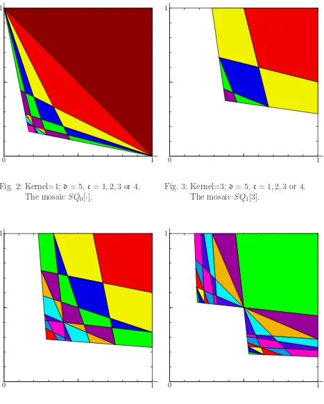
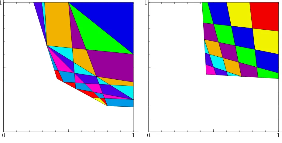
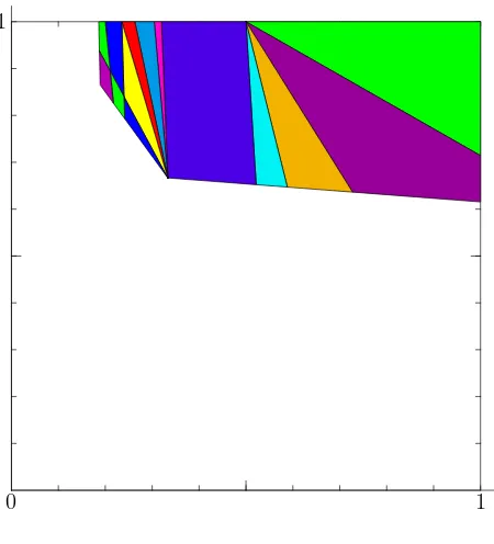
of each k to g1(x, y). The tiles of a given kernel fit into a few larger polygons, which we call mosaics. Their common feature is that always one of their vertices is at (1,1). They are either symmetric with respect to the first diagonal or they appear in pairs, symmetric to each other with respect to the first diagonal. Most of them are quadrangles, but their shape may vary a lot with d, c and the value of the kernel.
These mosaics behave like successive layers of constant density put over [0,1]2. Then the local density g1(x, y) at a given point (x, y) ∈ [0,1]2 is the sum of the densities on the mosaics (the inverse of its kernel) stung by (x, y). The contribution to the sum is halved if (x, y) touches only an edge of a mosaic, and if the point touches a vertex of a mosaic, it adds to the sum the density reduced proportionally with the size of the angle of the mosaic at that vertex. The number of mosaics that lay over (x, y)6= (1,1) is finite, and it is endless if (x, y) = (1,1).
For each given c,d, the number of the mosaics is unbounded, but their size has a certain rate of decay as their kernel increases. In the Appendix we have included the larger mosaics in two moduli: d= 5 and d= 12.
10
Acknowledgments
The authors are grateful to the referees for their very useful comments and suggestions.
11
Appendix–The Plane-mosaics in the cases
c
= 1
,
2
,
3
,
4;
d
= 5
and
c
= 3;
d
= 12
We have assigned names to the mosaics using the following conventions. The first letter is either S or N, according to whether the mosaic is or is not symmetric with respect to the first diagonal. Since the non-symmetric ones appear in pairs, symmetric to each other with respect to the first diagonal, we have included the picture of only one of them. The next letter or group of letters indicates the shape of the mosaic. The possible configuration are: triangle (T), quadrangle (Q), pentagon (P), hexagon (H), octagon (O) or concave hexagon– V-shape (V). The argument is the tuple k that gives the tile from the North-East corner. Finally, the subscript represents the number of components of k.
For example, the mosaic N P3[2,2,3] (see Figure 8) is a non-symmetric pentagon, whose tile from the N-E corner is the transformation of T2,2,3 through F3(x, y), and SQ1[6] (Fig-ure 15) is a symmetric quadrangle, whose piece from the N-E corner is the image of T6 throughF1(x, y).
As an exemplification, in Figure 1 we have included merely a tree associated with a mosaic. There, nodes are the tuples kdefining the tiles of N P3[2,2,3] and the arcs connect tuples kthat define adjacent tiles of the mosaic from Figure 8.
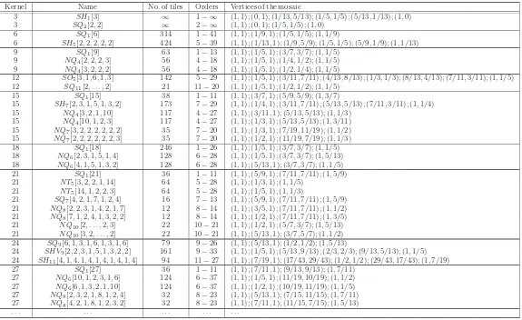
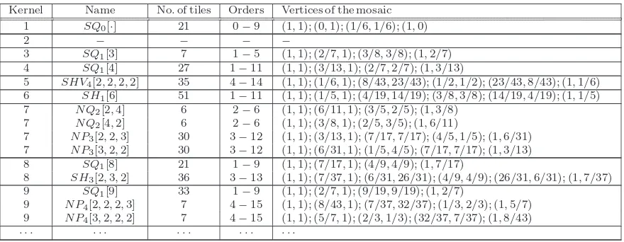
More data on the mosaics are entered in Tables 1 and 2. On the first column, one can find the kernel, the number whose inverse gives the local density on the layer given by that mosaic. The entry on the third column is the number of tiles arranged in the mosaic, while on the forth are the orders–the number of components–of k’s (the smallest and the largest) that produce the tiles. In the last column are the coordinates of the vertices of the mosaic.
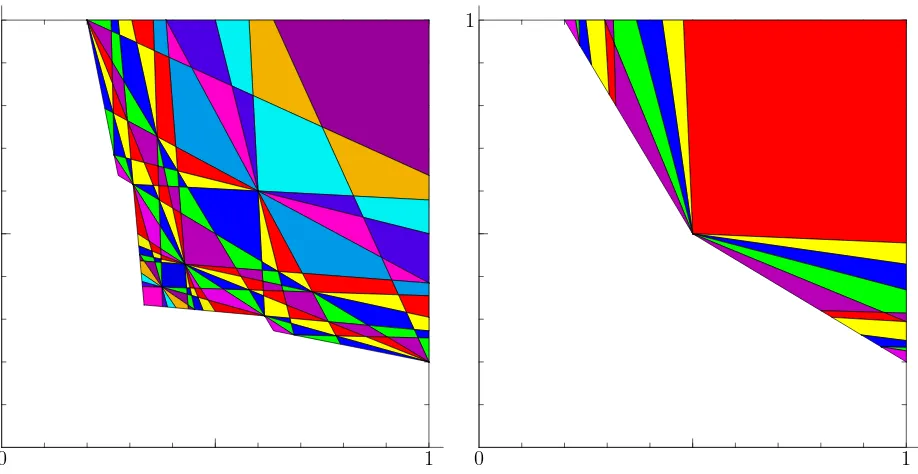
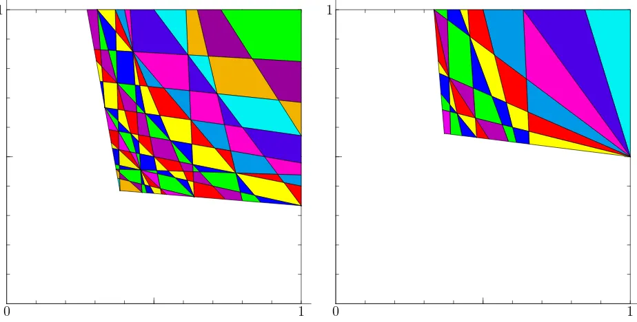
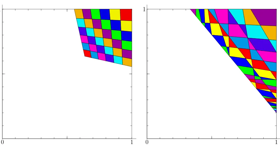
In the pictures we have used the same color to indicate the chains of tiles with k’s of the same orders. There, always neighbor chains have orders of k’s that differ by exactly one.
For the modulus d= 5, the mosaics are the same in any of the casesc= 1,2,3 or 4, but they are different when c = 0. When d = 12, the situation is more complex, mainly due to the larger number of factors of 12. Due to arithmetical constraints, there are no mosaics of kernel 2 when d= 5 and c= 1,2,3 or 4.
We remark that D1(c,5) = SQ0[·], for c = 1,2,3 or 4 and D1(3,12) = SH1[3]. In other words, this says that the limiting set of pairs of consecutive denominators from FQ(c,d) equals, as Q→ ∞, the largest of the mosaics.
Table 1: The mosaics in the casesd= 5,c= 1,2,3 or 4. Kernel Name No.of tiles Orders Vertices of the mosaic
1 SQ0[·] 21 0−9 (1,1); (0,1); (1/6,1/6); (1,0)
2 − − − −
3 SQ1[3] 7 1−5 (1,1); (2/7,1); (3/8,3/8); (1,2/7)
4 SQ1[4] 27 1−11 (1,1); (3/13,1); (2/7,2/7); (1,3/13)
5 SHV4[2,2,2,2] 35 4−14 (1,1); (1/6,1); (8/43,23/43); (1/2,1/2); (23/43,8/43); (1,1/6)
6 SH1[6] 51 1−11 (1,1); (1/5,1); (4/19,14/19); (3/8,3/8); (14/19,4/19); (1,1/5)
7 N Q2[2,4] 6 2−6 (1,1); (6/11,1); (3/5,2/5); (1,3/8)
7 N Q2[4,2] 6 2−6 (1,1); (3/8,1); (2/5,3/5); (1,6/11)
7 N P3[2,2,3] 30 3−12 (1,1); (3/13,1); (7/17,7/17); (4/5,1/5); (1,6/31)
7 N P3[3,2,2] 30 3−12 (1,1); (6/31,1); (1/5,4/5); (7/17,7/17); (1,3/13)
8 SQ1[8] 21 1−9 (1,1); (7/17,1); (4/9,4/9); (1,7/17)
8 SH3[2,3,2] 36 3−13 (1,1); (7/37,1); (6/31,26/31); (4/9,4/9); (26/31,6/31); (1,7/37)
9 SQ1[9] 33 1−9 (1,1); (2/7,1); (9/19,9/19); (1,2/7)
9 N P4[2,2,2,3] 7 4−15 (1,1); (8/43,1); (7/37,32/37); (1/3,2/3); (1,5/7)
9 N P4[3,2,2,2] 7 4−15 (1,1); (5/7,1); (2/3,1/3); (32/37,7/37); (1,8/43)
13
2 2 3
2 3 1 4
3 1 4 1 4 2 3 1 5 1
1 4 1 4 1 4 3 1 4 1 5 1 2 3 1 6 1 2
1 2 4 1 4 1 4 1 4 1 4 1 5 1 3 1 4 2 1 6 1 2 3 2 1 7 1 2 2 3 1 6 1 3 1
1 3 1 5 1 4 1 4 1 4 1 4 2 1 6 1 3 1 4 2 1 7 1 2 2 3 2 1 7 1 3 1
1 4 1 5 1 3 1 6 1 3 1 5 1 3 1 7 1 2 3 1 4 2 1 7 1 3 1 2 3 2 1 8 1 2 3 1
1 4 2 1 6 1 3 1 6 1 1 4 1 5 1 3 1 7 1 2 3 1 5 1 3 1 7 1 3 1 3 1 4 2 1 8 1 2 3 1 2 3 2 1 8 1 2 3 2 1
1 4 2 1 6 1 3 1 7 1 2 1 4 1 5 1 3 1 7 1 3 1 3 1 5 1 3 1 8 1 2 3 1 3 1 4 2 1 8 1 2 3 2 1
[image:13.792.68.719.113.508.2]14
Kernel Name No.of tiles Orders Vertices of the mosaic
3 SH1[3] ∞ 1− ∞ (1,1); (0,1); (1/13,5/13); (1/5,1/5); (5/13,1/13); (1,0)
3 SQ2[2,2] ∞ 2− ∞ (1,1); (0,1); (1/5,1/5); (1,0)
6 SQ1[6] 314 1−41 (1,1); (1/9,1); (1/5,1/5); (1,1/9)
6 SH5[2,2,2,2,2] 424 5−39 (1,1); (1/13,1); (1/9,5/9); (1/5,1/5); (5/9,1/9); (1,1/13)
9 SQ1[9] 63 1−13 (1,1); (1/5,1); (3/7,3/7); (1,1/5)
9 N Q4[2,2,2,3] 56 4−18 (1,1); (1/5,1); (1/4,1/2); (1,1/5)
9 N Q4[3,2,2,2] 56 4−18 (1,1); (1/5,1); (1/2,1/4); (1,1/5)
12 SO5[3,1,6,1,3] 142 5−29 (1,1); (1/5,1); (3/11,7/11); (4/13,8/13); (1/3,1/3); (8/13,4/13); (7/11,3/11); (1,1/5)
12 SQ11[2, . . . ,2] 21 11−20 (1,1); (1/5,1); (1/2,1/2); (1,1/5)
15 SQ1[15] 38 1−11 (1,1); (3/7,1); (5/9,5/9); (1,3/7)
15 SH7[2,3,1,5,1,3,2] 173 7−29 (1,1); (1/4,1); (3/11,7/11); (5/13,5/13); (7/11,3/11); (1,1/4)
15 N Q4[3,2,1,10] 117 4−27 (1,1); (3/11,1); (5/13,5/13); (1,1/3)
15 N Q4[10,1,2,3] 117 4−27 (1,1); (1/3,1); (5/13,5/13); (1,3/11)
15 N Q7[3,2,2,2,2,2,2] 35 7−20 (1,1); (1/3,1); (7/19,11/19); (1,1/2)
15 N Q7[2,2,2,2,2,2,3] 35 7−20 (1,1); (1/2,1); (11/19,7/19); (1,1/3)
18 SQ1[18] 246 1−26 (1,1); (1/5,1); (3/7,3/7); (1,1/5)
18 N Q6[2,3,1,5,1,4] 128 6−28 (1,1); (1/5,1); (3/7,3/7); (1,5/13)
18 N Q6[4,1,5,1,3,2] 128 6−28 (1,1); (5/13,1); (3/7,3/7); (1,1/5)
21 SQ1[21] 36 1−11 (1,1); (5/9,1); (7/11,7/11); (1,5/9)
21 N T5[3,2,2,1,14] 64 5−28 (1,1); (1/3,1); (1,1/5)
21 N T5[14,1,2,2,3] 64 5−28 (1,1); (1/5,1); (1,1/3)
21 SQ7[4,2,1,7,1,2,4] 16 7−13 (1,1); (5/9,1); (7/11,7/11); (1,5/9)
21 N Q8[2,2,3,1,4,2,1,7] 12 8−14 (1,1); (3/5,1); (7/11,7/11); (1,1/2)
21 N Q8[7,1,2,4,1,3,2,2] 12 8−14 (1,1); (1/2,1); (7/11,7/11); (1,3/5)
21 N Q10[2, . . . ,2,3] 22 10−21 (1,1); (1/2,1); (5/7,3/7); (1,5/13)
21 N Q10[3,2, . . . ,2] 22 10−21 (1,1); (5/13,1); (3/7,5/7); (1,1/2)
24 SQ9[6,1,3,1,6,1,3,1,6] 79 9−26 (1,1); (5/13,1); (1/2,1/2); (1,5/13)
24 SHV9[2,2,3,1,5,1,3,2,2] 161 9−33 (1,1); (1/5,1); (5/13,9/13); (2/3,2/3); (9/13,5/13); (1,1/5)
24 SH11[4,1,4,1,4,1,4,1,4,1,4] 94 11−27 (1,1); (7/19,1); (17/43,29/43); (1/2,1/2); (29/43,17/43); (1,7/19)
27 SQ1[27] 36 1−11 (1,1); (7/11,1); (9/13,9/13); (1,7/11)
27 N Q6[10,1,2,3,1,6] 124 6−37 (1,1); (1/5,1); (11/19,10/19); (1,1/2)
27 N Q6[6,1,3,2,1,10] 124 6−37 (1,1); (1/2,1); (10/19,11/19); (1,1/5)
27 N Q8[2,3,2,1,8,1,2,4] 32 8−23 (1,1); (5/13,1); (7/15,11/15); (1,7/11)
27 N Q8[4,2,1,8,1,2,3,2] 32 8−23 (1,1); (7/11,1); (11/15,7/15); (1,5/13)
[image:14.792.114.689.87.439.2]References
[1] E. Alkan, A. H. Ledoan, A. Zaharescu, A parity problem on the free path length of a billiard in the unit square with pockets, preprint.
[2] F. P. Boca, C. Cobeli, A. Zaharescu, On the distribution of the Farey sequence with odd denominators, Michigan Math. J., 51 (2003), 557–573.
[3] F. P. Boca, R. N. Gologan, A. Zaharescu, The average length of a trajectory in a certain billiard in a flat two-torus, New York J. Math. 9 (2003), 303–330.
[4] F. P. Boca, R. N. Gologan, A. Zaharescu, The statistics of the trajectory of a certain billiard in a flat two-torus, Commun. Math. Phys. 240 (2003), no. 1–2, 53–73.
[5] F. P. Boca, R. N. Gologan, A. Zaharescu, Sur le mod´ele du gaz de Lorentz p´eriodique,
An. Univ. Craiova Ser. Mat. Inform. 30 (2003), no. 1, 63–70.
[6] F. P. Boca and A. Zaharescu, Farey fractions and two-dimentional tori, in Noncom-mutative Geometry and Number Theory (C. Consani, M. Marcolli, eds.), Aspects of Mathematics E37, Vieweg Verlag, Wiesbaden, 2006, 57–77.
[7] J. Bourgain, F. Golse, and B. Wennberg, On the distribution of free path lengths for the periodic Lorentz gas, Commun. Math. Phys. 190 (1998), 491–508.
[8] L. A. Bunimovich, Billiards and other hyperbolic systems, in Ya G. Sinaie et al., eds.,
Dynamical Systems, Ergodic Theory and Applications,Encyclopaedia of Math. Sci.100, 2nd ed., Springer-Verlag, Berlin, 2000, pp. 192–233.
[9] C. Cobeli, A. Zaharescu, The Haros-Farey sequence at two hundred years, Acta Univ. Apulensis Math. Inform. 5 (2003), 1–38.
[10] C. Cobeli, A. Iordache, A. Zaharescu, The relative size of consecutive odd denominators in Farey series, Integers, 3, A7, (2003), 14 pp. (electronic).
[11] C. Cobeli, A. Zaharescu, A density theorem on even Farey fractions, preprint.
[12] C. Cobeli, A. Zaharescu, On the small neighbor denominators of the Farey series with denominators in arithmetic progression, preprint.
[13] A. Haynes, A note on Farey fractions with odd denominators, J. Number Theory 98
(2003), 89–104.
[14] A. Haynes, The distribution of special subsets of the Farey sequence,J. Number Theory
107 (2004), 95–104.
2000 Mathematics Subject Classification: Primary 11B57.
Keywords: Farey fractions, arithmetic progressions, congruence constraints.
Received September 15 2004; revised version received May 20 2005; July 20 2006. Published inJournal of Integer Sequences, July 20 2006.
0 1 1
Fig. 2: Kernel=1; d= 5, c= 1,2,3 or 4. The mosaic SQ0[·].
0 1
1
Fig. 3: Kernel=3; d= 5, c= 1,2,3 or 4. The mosaic SQ1[3].
0 1
[image:17.612.75.537.404.644.2]1
Fig. 4: Kernel=4; d= 5, c= 1,2,3 or 4. The mosaic SQ1[4].
0 1
1
0 1 1
Fig. 6: Kernel=6; d= 5, c= 1,2,3 or 4. The mosaic SH1[6].
0 1
1
Fig. 7: Kernel=7; d= 5, c= 1,2,3 or 4. The mosaic N Q2[2,4].
0 1
[image:18.612.74.538.411.647.2]1
Fig. 8: Kernel=7; d= 5, c= 1,2,3 or 4. The mosaic N P3[2,2,3].
0 1
1
0 1 1
Fig. 10: Kernel=8; d= 5, c= 1,2,3 or 4. The mosaic SH3[2,3,2].
0 1
1
Fig. 11: Kernel=9; d= 5, c= 1,2,3 or 4. The mosaic SQ1[9].
0 1
[image:19.612.192.417.416.664.2]1
0 1 1
Fig. 13: Kernel=3; d= 12, c= 3. The mosaic SH1[3].
0 1
1
Fig. 14: Kernel=3; d= 12, c= 3. The mosaic SQ2[2,2].
0 1
[image:20.612.75.537.404.643.2]1
Fig. 15: Kernel=6; d= 12, c= 3. The mosaic SQ1[6].
0 1
1
0 1 1
Fig. 17: Kernel=9; d= 12, c= 3. The mosaic SQ1[9].
0 1
[image:21.612.75.537.82.325.2]1
Fig. 18: Kernel=9; d= 12, c= 3. The mosaic N Q4[2,2,2,3].
0 1
1
Fig. 19: Kernel=12; d= 12, c= 3. The mosaic SO5[3,1,6,1,3].
0 1
[image:21.612.79.538.405.642.2]1
0 1 1
Fig. 21: Kernel=15; d= 12, c= 3. The mosaic SQ1[15].
0 1
1
Fig. 22: Kernel=15; d= 12, c= 3.
The mosaic SH7[2,3,1,5,1,3,2].
0 1
1
Fig. 23: Kernel=15; d= 12, c= 3. The mosaic N Q4[3,2,1,10].
0 1
[image:22.612.70.543.201.623.2]1
Fig. 24: Kernel=15; d= 12, c= 3.
[image:22.612.75.537.408.642.2]0 1 1
Fig. 25: Kernel=18; d= 12, c= 3. The mosaic SQ1[18].
0 1
[image:23.612.75.538.81.326.2]1
Fig. 26: Kernel=18; d= 12, c= 3. The mosaic N Q6[2,3,1,5,1,4].
0 1
[image:23.612.76.538.400.649.2]1
Fig. 27: Kernel=21; d= 12, c= 3. The mosaic SQ1[21].
0 1
1
0 1 1
Fig. 29: Kernel=21; d= 12, c= 3.
The mosaic SQ7[4,2,1,7,1,2,4].
0 1
[image:24.612.72.539.101.580.2]1
Fig. 30: Kernel=21; d= 12, c= 3.
The mosaic N Q8[2,2,3,1,4,2,1,7].
0 1
[image:24.612.77.537.411.642.2]1
Fig. 31: Kernel=21; d= 12, c= 3. The mosaic N Q10[2, . . . ,2,3].
0 1
1
Fig. 32: Kernel=24; d= 12, c= 3.
0 1 1
Fig. 33: Kernel=24; d= 12, c= 3.
SHV9[2,2,3,1,5,1,3,2,2].
0 1
1
Fig. 34: Kernel=24; d= 12, c= 3.
SH11[4,1,4,1,4,1,4,1,4,1,4]
0 1
[image:25.612.76.537.81.324.2]1
Fig. 35: Kernel=27; d= 12, c= 3. The mosaic SQ1[27].
0 1
1
[image:25.612.77.538.408.649.2]0 1 1
Fig. 37: Kernel=27; d= 12, c= 3.
![Fig. 1: The tree of k’s associated with the mosaic NP3[2, 2, 3] (c = 1, 2, 3 or 4 and d = 5).](https://thumb-ap.123doks.com/thumbv2/123dok/927928.903626/13.792.68.719.113.508/fig-tree-k-s-associated-mosaic-np-c.webp)